3.1. Application to Grid-Connected PV Systems
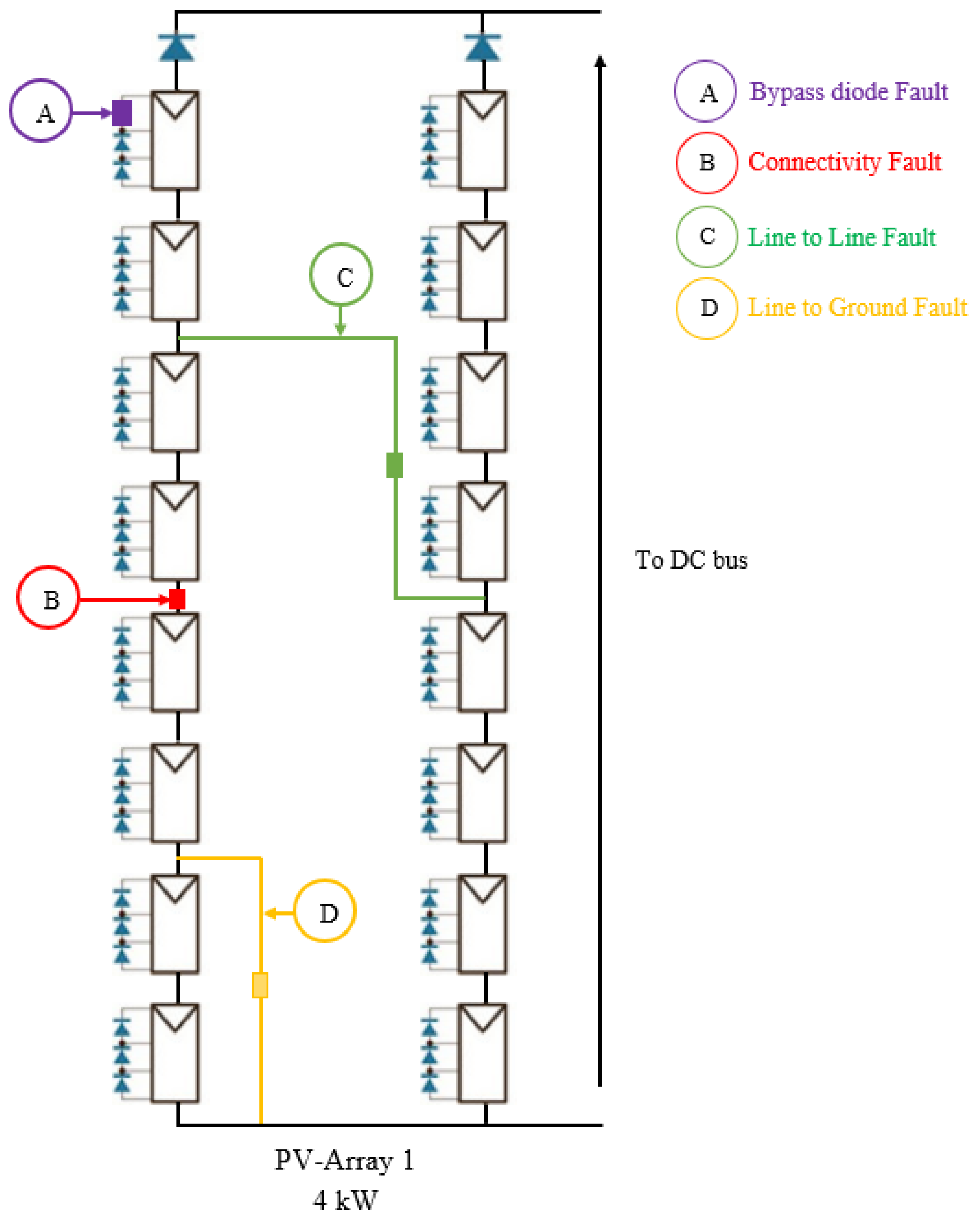
Figure 5 presents a PV system configuration with a DC bus voltage of 500 (V). The PV side consists of three PV arrays delivering a maximum power of 4 kW each. A single PV array set consists of 2 parallel strings where each string has 24 modules connected in series. Each module contains 20 cells (see
Figure 6).
In this work, we injected different scenarios in the PV1 and PV2 systems, which included five types of faults, as indicated in
Table 1:
A simple fault in
contains four scenarios of faults, A bypass diode fault (fault1) is emulated by varying the resistance. The connectivity fault (fault2) is considered in string 1, between two modules. fault2 is modeled by a serial variable resistance (Rf2) at one point. The resistance variation represents the state of the considered fault. The two faults line-to-line fault and line-to-ground fault (fault3 and fault4) are described by the variation in the resistances Rf3 and Rf4, respectively. Rf3 is located between two different points, and Rf4 is located between one point and the ground. Resistive faults with
equal to 0 and infinity are considered for fault1 and fault2. In fault3 and fault4, resistive faults equal to 10 and 20 (
) are settled. As shown in
Figure 6, 16 different scenarios can be generated from those four faults.
The same simple faults are injected in PV2.
The second scenario is about multiple faults, which present more than onefault in one PV, injected in PV1 and PV2.
Finally, mixed faults represent several faults in both PVs at the same time.
Experimental data variables were collected to prepare for the various tests performed for fault classification purposes. The PV healthy state is classified as class
, whereas the other 16 operating modes are classified as classes
, respectively. The dataset collected from the PV system was divided into two subsets; training (4000 samples) and testing (200 samples) (please refer to
Table 2).
Table 3 contains a variety of simulated variables that are needed to carry out the various tests for FDD.
3.3. Fault Classification Results
To obtain classification accuracy and demonstrate the efficacy of the presented methodologies for FDD purposes, a 10-fold cross-validation approach was adopted, and we chose 50 as the Maxepochs with 10 Hiddens. The healthy operation was assigned to class , while the 16 faulty modes (–) were assigned to classes –.
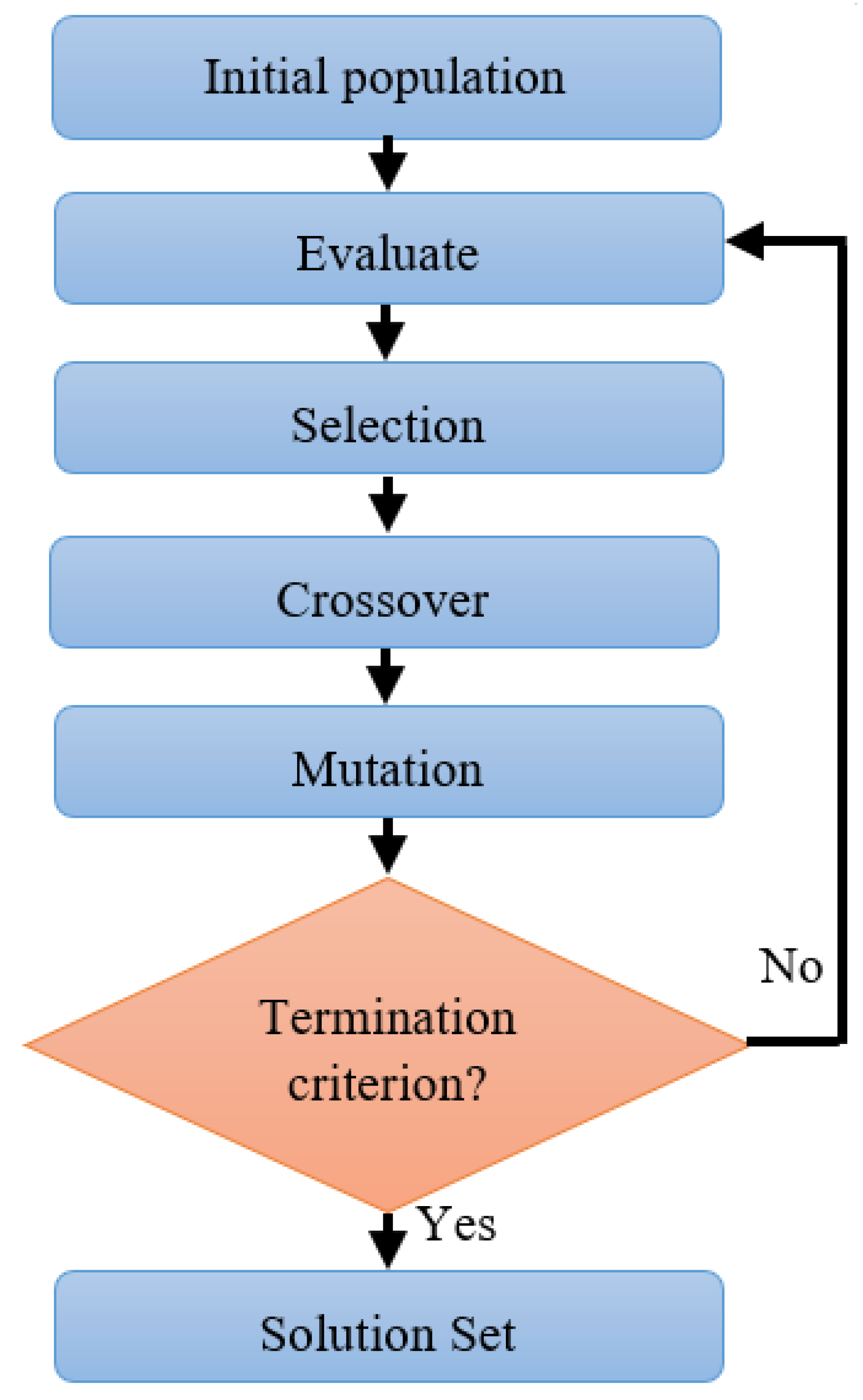
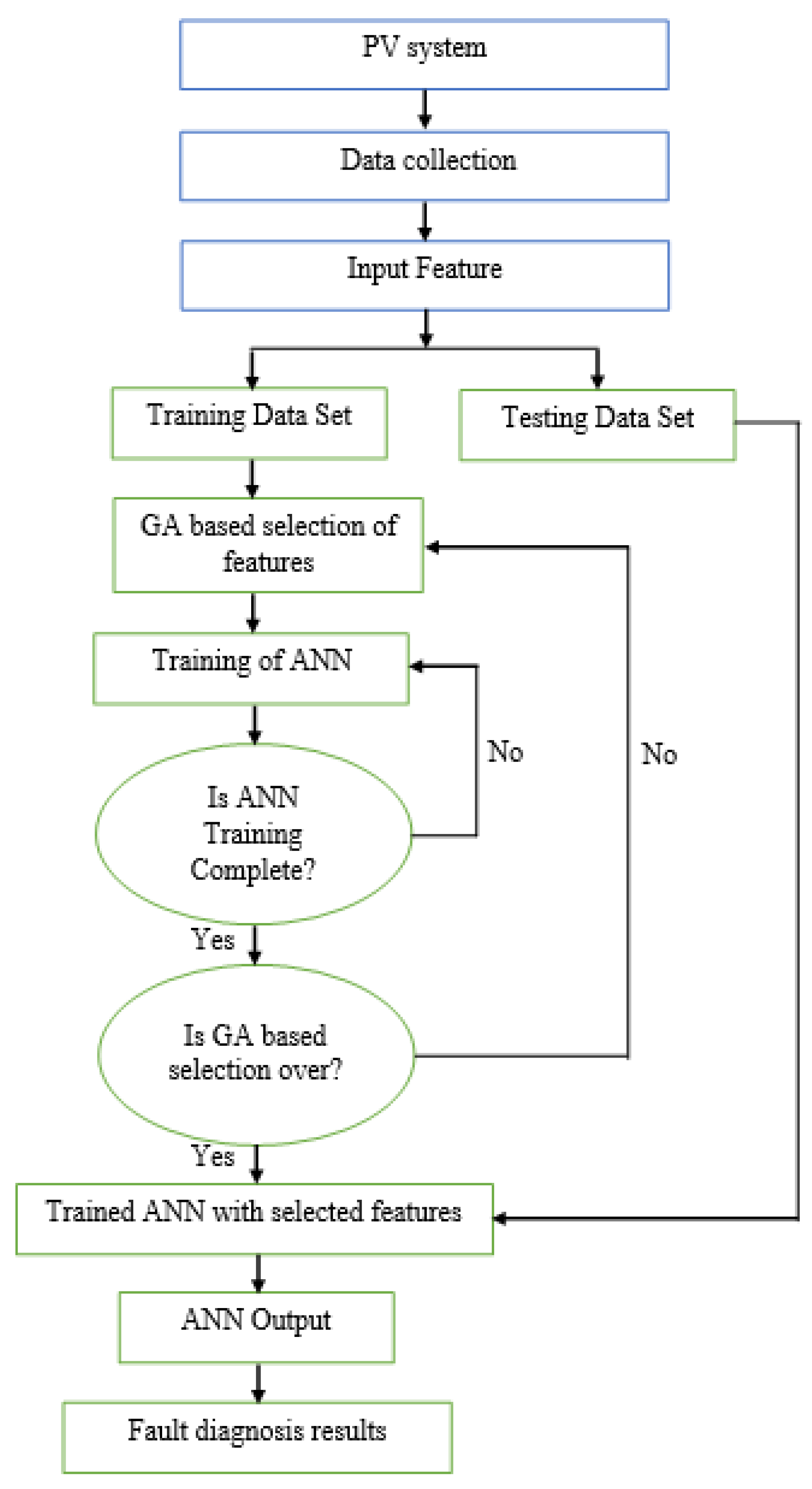
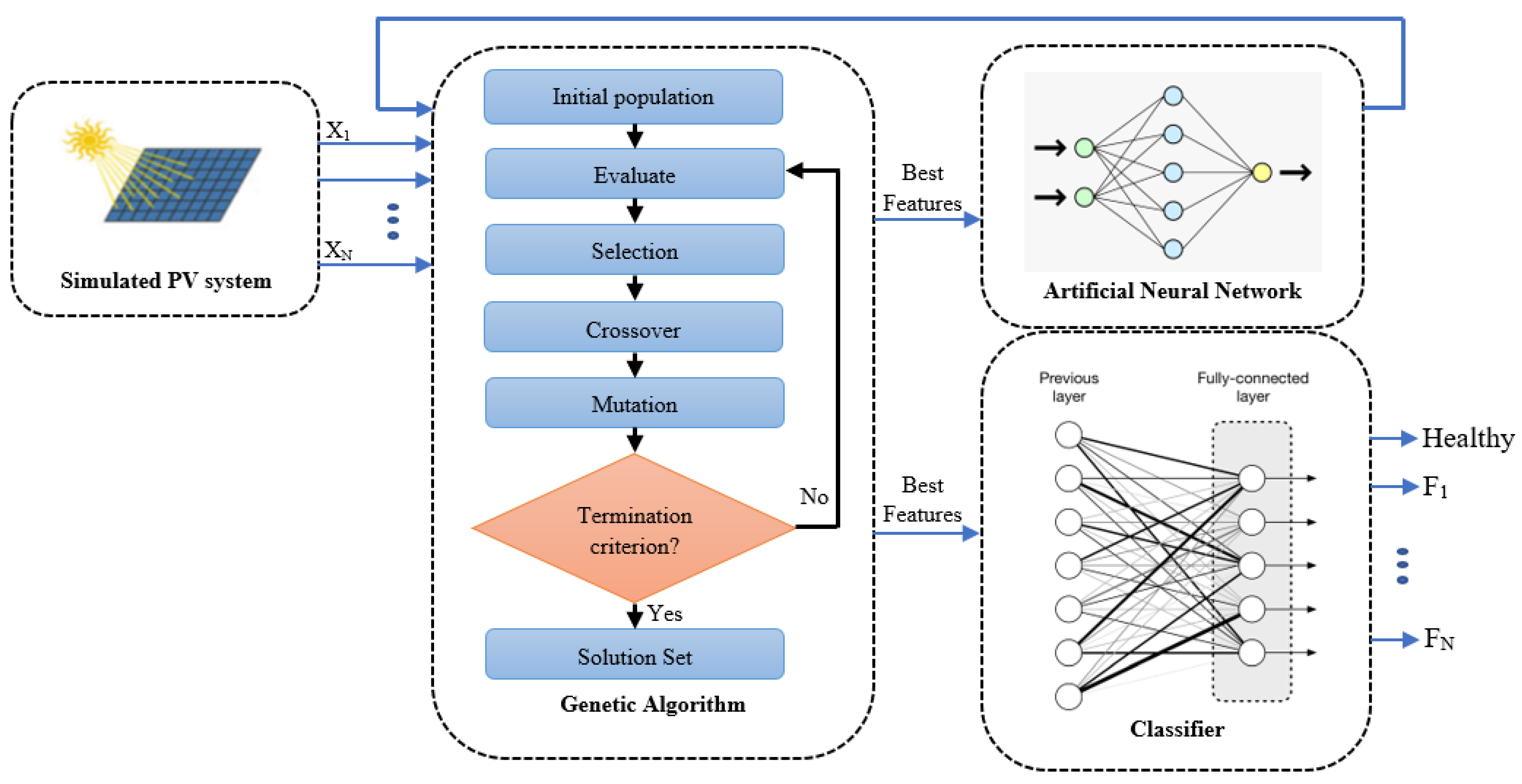
In the first stage, PV data were applied to collect and label the database in faulty mode. Then, we used the labeled data as inputs for the presented approaches. The main idea of the ANN-based GA is to decrease the computational time of the ANN model. A confusion matrix is offered to further highlight the diagnostic performance of the proposed approaches (see
Table 4 and
Table 5). The confusion matrix is a visual representation of the proposed algorithms’ performance. The columns represent instances in a predicted class, while the rows represent occurrences in an actual class. In addition, the confusion matrix shows which samples were correctly identified and which were misclassified for each condition mode (
to
) for the GCPV system. The two proposed algorithms identify 2000 samples among 2000 for the healthy case in the GCPV systems, which is attributed to class
(true positive). Furthermore, the detection precision and recall are also
. As a result, this class has no misclassification.
Table 4, which presents the confusion matrix of the proposed ANN method in the GCPV system, shows that, for the faulty case (
), the precision is
and the recall is
. In this case, 354 samples are identified as fault10 among 2000 assigned to class
. For the faulty case (
), the precision is
and the recall is
. In this case, 488 samples are identified as fault3 among 2000 assigned to class
. For the faulty case (
), the precision is
and the recall is
. In this case, 1566 samples are identified as fault1 among 2000 assigned to class
. Finally, for the faulty case (
), the precision is
and the recall is
. In this case, 2000 samples are identified as fault6.
Table 5m which presents the confusion matrix of the proposed NN-based GA in the GCPV system shows that for the faulty case (
), the precision is
and the recall is
. In this case, 449 samples are identified as fault10 among 2000 assigned to class
. For the faulty case (
), the precision is
and the recall is
. In this case, 972 samples are identified as fault3 among 2000 assigned to class
. For the faulty case (C10), the precision is
and the recall is
. In this case, 1299 samples are identified as fault1 among 2000 assigned to class
. Finally, for the faulty case (
), the precision is
and the recall is
. In this case, 164 and 1031 samples are identified as fault6 and fault7 among 2000 assigned to class
and
.
The performance of the proposed NN and NN-based GA approaches is shown in
Table 6. Furthermore, as compared to the NN with the GA method, the computation time is decreased by more than
while maintaining about the same accuracy. Applying the GA shows that the number of input features is decreased; from 8 features (variables), we obtain just 2 important ones (1,2), which presents the simple and multiple faults in PV1. Furthermore, we note that the computation time is decreased as well, from 0.28 s to 0.15 s, while it maintains almost the same accuracy from
to
. The next scenario in PV2, the number of features (3,4) and the computation time are reduced, although the accuracy keeps the same values. Regarding the third one, the number of features is decreased as well; it provides 4 variables (1,2,3,4) from 8 features. It provides the same accuracy, precision, and recall:
; at the same time, it minimizes the computation time from 0.30 s to 0.20 s. The last scenario looks like the previous one, reducing the number of variables from 8 to 4 features (1,2,3,4)f, which presents all faults, and the accuracy is almost the same:
to
. In addition, the computation time is reduced from 0.98 s to 0.40 s.
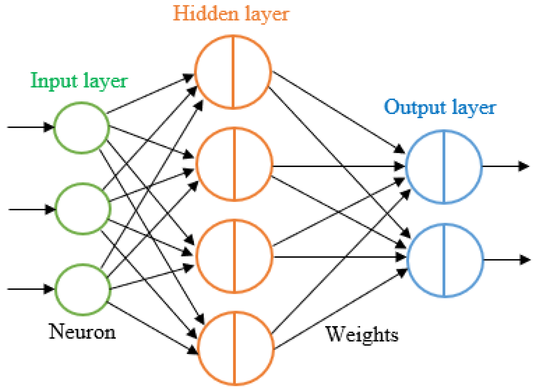
To validate the robustness and effectiveness of our method, we propose other classifiers such as the recurrent neural network (RNN), long short-term memory (LSTM), convolution neural network (CNN), feed forward neural network (FFNN), and cascade forward neural network (CFNN).
The architecture of the CNN developed in this work is composed of 26 layers: input layer, six convolution layers, five batch normalization layers, five max pooling layers, six ReLU layers, fully connected layer, sotfmax layer, and output layer. The number of filters used in the convolutional layers is 8, 16, 32, 64, 128, and 256, respectively. Each convolutional layer is followed by a batch normalization layer. A fully connected dense layer having six nodes with the softmax activation follows the max pooling block. We set 50 epochs and 250 as the miniBatchsize for our network. We used “ReLU” as the activation function.
The architecture of the proposed LSTM is composed of ten layers: an input layer, 3 LSTM hidden layers, 3 dropout layers, a fully connected layer, a softmax layer, and an output layer. The LSTM layers are composed of three hidden layers with 50 nodes in the first layer, 10 nodes in the second layer, and 6 nodes in the third layer. The fully connected layer is composed of six nodes.
In the architecture of the RNN, we chose 50 epochs as the Maxepochs with 10 Hiddens.
In the architecture of the FFNN, we chose 50 epochs as the Maxepochs with 10 Hiddens.
Finally, in the architecture of the FFNN, we chose 50 epochs as the Maxepochs with 10 Hiddens.
Table 7 summarizes the performances of the proposed method. The LSTM and CNN showed that the computation time is reduced and maintains almost the same accuracy, recall, and precision: 5.05 s to 2.84 s for LSTM, 6.2 s to 4.42 s for CNN, 0.85 s to 0.23 s for FFNN, and 0.64 s to 0.20 s for CFNN. In addition to the RNN, which provides an accuracy from 61.82% to 64.70%, it reduces the computation time by more than 50%.
