Data-Driven Robust DEA Models for Measuring Operational Efficiency of Endowment Insurance System of Different Provinces in China

Abstract

China is facing an increasingly serious aging problem, which puts forward higher requirements for the smoothness of the endowment insurance system. Accurate evaluation of the efficiency of the system can help the government to find problems and improve the system. Some scholars have used data envelopment analysis (DEA) method to measure the efficiency of endowment insurance system. However, according to the literature, the impact of government policy adjustment and economic shocks on output of the data was ignored. In this study, a robust optimization method is applied to deal with uncertainty. Robust DEA models proposed in this paper are based on three kinds of uncertainty sets. A data-driven robust optimization method is also applied to resolve the over-conservative problem. Compared with the robust DEA method, based on analysis it is found that the data-driven robust DEA method is more flexible and reliable for efficiency estimating strategies. The results of data-driven robust DEA models illustrate that the government should increase its support for the endowment insurance system, especially for the underdeveloped regions.

1. Introduction

In recent years, China’s aging process has been accelerating. By October 2020, China’s population aged 60 or above reached 264 million, accounting for 18.7% of the total population, of which 191 million will be aged 65 or above, accounting for 13.5% of the total population [1]. The research shows that China will enter a moderately aging society by 2024, with 14% of the population over 65 years old. According to research, China will enter into the serious aging society by 2035 and the proportion of the elderly population over 65 will be increased by more than 20%. In the past few decades, China has moved from the demographic dividend period to the population burden period [2]. The cruel reality of getting old before getting rich will bring a great burden to young people, and will also pose the most severe challenge to the current endowment insurance system. Evaluation of the operation process and effects of the current endowment insurance system objectively and scientifically has become an urgent problem for the further improvement and development of the endowment insurance system. It creates a great significance to grasping the operation status of the endowment insurance system and promoting its sustainable development.

Research on the efficiency of insurance system began as early as the 1950s. Samuelson proposed the Overlapping Generation Model (OLG) to study the performance of endowment insurance [3]. Later, Diamond improved the OLG model, he used the model to study the dynamic impact of two existing financing modes of endowment insurance system on capital [4]. In the 1970s, Aaron proposed the ‘Aaron condition’, which became a reference standard for the choice of a pension insurance system. He found that the main factors restricting the efficiency of endowment insurance are the growth rate of population and the growth rate of labor production [5]. In recent years, some scholars have studied China’s maternity insurance system and basic pension insurance system [6,7]. However, there is little research on endowment insurance systems in China. Charnes et al. proposed that DEA is the most popular non-parametric method to measure the relative efficiency of decision-maker units, and it was developed later on by Banker et al. [8,9]. The DEA method is widely used among various fields: Bank [10,11,12], energy [13,14,15,16], educational system [17,18], entrepreneurship and innovation [19,20], software engineering [21,22]. Andreu proposed four variants of the slacks-based measure of efficiency (SBM) to evaluate the efficiency of the strategic style of pension funds [23]. Further, Hu improved the three-stage DEA model to calculate the operation efficiency of urban and rural residential insurance system in 31 provinces of China from 2012 to 2016, he proposed that different regions should implement different efficiency promotion strategies according to their own problems and situation [24].

With the deepening of population aging, the gap in endowment insurance system is becoming increasingly serious, which means that the consumption of accumulated pension balance will be increased. The change of population structure promotes the change of relevant national policies, it also has an impact on the pension payment rate. Moreover, the stable operation of the economy is very important for the sustainable operations of the endowment insurance system. In case of economic crisis, the accumulated pension balance will be affected. Hence, there are sufficient reasons to believe that the accumulated pension balance and pension expenditures are in an uncertain environment, and this uncertainty is caused by a variety of factors such as economic shock and adjustment of the policy. In previous studies, few scholars consider this uncertainty, likely to lead to wrong ranking results.

Robust Optimization is introduced in this study to resolve the problems mentioned above. It was first proposed by Soyster [25]. El-Ghaoui and Lebret [26] and Ben-Tal and Nemirovski [27,28,29] extended the RO theory and proposed a new robust model based on ellipsoidal uncertainty sets. Subsequently, Bertsimas and Sim [30,31,32] and Bertsimas et al. [33] developed a robust optimization approach based on polyhedral uncertainty sets. Sadjadi and Omrani were the first scholars to apply robust optimization for DEA [34]. Kazemia and Haji proposed robust DEA model based on Ben-Tal and Bertsimas approaches to measure the efficiency of high schools [35]. Until now, no scholar has used the robust DEA method to resolve the problems in the field of endowment insurance systems.

However, it is highly subjective that the classical RO methods are mostly based on experience to obtain uncertainty sets. In previous studies, the advantages of big data are ignored, and the results are also too conservative. The data-driven RO method [36,37] uses historical data to construct uncertainty sets, which improves the rationality and economy of the uncertainty sets of the traditional RO method. However, few types of research were conducted previously on introducing data-driven RO to DEA models.

In this paper, a new method is proposed to measure the efficiency of endowment insurance system of 31 provinces in China under uncertainty environment. It is proposed to use a data-driven robust data envelopment analysis (DRDEA) model. It is based on three uncertainty sets: Interval uncertainty set, Ellipsoid uncertainty set, Polyhedron uncertainty set. The determination of the government is to ensure that the operation of the endowment insurance system should be absolutely stable, so the purpose was to resort robust optimization to ensure robustness in the case of data disturbance. The main contributions of this research are as follows: (1) It is proposed that robust DEA models deal with the efficiency measurement in endowment insurance effectively. (2) We deduce the robust counterparts in different deterministic cases. (3) It is proposed that data-driven robust DEA models deal with the inherent defects of robust optimization. (4) This paper uses real numbers to verify the effectiveness of the model.

The structure of this paper is as follows. Section 2 introduces some preliminary concepts. Three robust DEA models are explained in Section 3. Section 4 highlights applicability of models mentioned earlier with endowment insurance system in China along with suggestions and recommendations. Section 5 elaborates the data-driven robust DEA models and its application in endowment insurance system. At the end, Section 6 reflects the conclusion of this paper.

2. Preliminaries

In this section, related knowledge about DEA and Interval DEA theory is presented.

2.1. Data Envelopment Analysis

Data envelopment analysis (DEA) was first proposed by Charnes et al. to measure the relative efficiency [8]. Suppose we have $n$ homogeneous decision-making units ($DM{U}_s$). Here, for each $DM{U}_j$, it consumes $m$ inputs (fund income, the number of insured and the number of retirees) that are denoted by $x_{ij}$ and produces $s$ outputs (fund expenditure and accumulated fund balance) which are denoted by $y_{rj}$. Then, we obtain the following model:

$$\begin{array}{ll}\max \theta =& \frac{{\displaystyle \sum _{r=1}^s{u}_r{y}_{ro}}}{{\displaystyle \sum _{i=1}^m{v}_i{x}_{io}}}\\ s.t.& \frac{{\displaystyle \sum _{r=1}^s{u}_r{y}_{rj}}}{{\displaystyle \sum _{i=1}^m{v}_i{x}_{ij}}}\le 1,{\forall }_j\\ & u_r,v_i\ge 0.\end{array}$$

(1)

Obviously, model (1) is a fractional programming. Charnes–Cooper transformation can be used to obtain a linear programming [6]:

$$\begin{array}{ll}\max \theta =& {\displaystyle \sum _{r=1}^S{u}_{r}y}\\ s.t.& {\displaystyle \sum _{i=1}^m{v}_i{x}_{io}^{}}\le 1\\ & {\displaystyle \sum _{r=1}^S{u}_r{y}_{rj}^{}}-{\displaystyle \sum _{i=1}^m{v}_i{x}_{ij}^{}}\le 0,{\forall }_j \\ & u_r,v_i\ge 0.\end{array}$$

(2)

Here, $\theta$ represents the efficiency of decision-making units. At the same time, we use “≤” in our DEA model instead of “=” in the standard DEA model. The reason why we make this change is to avoid any infeasibility [38].

2.2. Interval DEA Model

This subsection introduces an Interval DEA model, that is, the ratio of all possible comprehensive inputs and comprehensive outputs of the DMU as all possible efficiency values, so the efficiency value obtained is presented as an interval form. We assume that the upper bounds and lower bounds of output are $y_{ij}^U$ and $y_{ij}^L$, respectively.

Firstly, we consider the most favorable situation for objective DMU. Let the output of objective DMU take the maximum value, and the output of other DMUs take the minimum value, so that the model of the upper bound of interval efficiency value can be obtained.

$$\begin{array}{ll}\max {\theta }^U=& {\displaystyle \sum _{r=1}^S{u}_r{y}_{ro}^U}\\ s.t.& {\displaystyle \sum _{i=1}^m{v}_i{x}_{io}^L}\le 1\\ & {\displaystyle \sum _{r=1}^S{u}_r{y}_{rj}^L}-{\displaystyle \sum _{i=1}^m{v}_i{x}_{ij}^U}\le 0,{\forall }_j \\ & u_r,v_i\ge 0.\end{array}$$

(3)

Similarly, considering the most unfavorable situation, the model of the lower bound of interval efficiency value can be obtained:

$$\begin{array}{ll}\max {\theta }^L=& {\displaystyle \sum _{r=1}^S{u}_r{y}_{ro}^L}\\ s.t.& {\displaystyle \sum _{i=1}^m{v}_i{x}_{io}^U}\le 1\\ & {\displaystyle \sum _{r=1}^S{u}_r{y}_{rj}^U}-{\displaystyle \sum _{i=1}^m{v}_i{x}_{ij}^L}\le 0,{\forall }_j \\ & u_r,v_i\ge 0.\end{array}$$

(4)

When we use the maximum value of input and the minimum value of output in model (3), the result is the lowest value of efficiency. In contrast, we obtain the maximum value of efficiency in model (4), that is to say $\theta \in [{\theta }^L,{\theta }^U]$.

3. Robust DEA Model

In this model (2), decision variables and parameters are all deterministic. However, in a real-world scenario, this is likely to lead to errors when uncertain factors exist. In our research, the operational efficiency of the endowment insurance system will be affected by policy adjustments and economic shocks. Therefore, the DEA model under certain circumstances is not suitable for real situations. We must consider the impact of these two uncertainties on output.

Robust optimization is an approach which is seeking the optimal solution in the worst case. In this paper, three uncertainty sets to describe the uncertainty were considered to describe different kinds of uncertainties which may influence the results.

For the output, it consists of two parts. The first part is determinate value, the other part is uncertainty value. We express the uncertainty as follows:

$$U=\{y_{ro}^D=y_{ro}+{\displaystyle \sum _{l=1}^L{y}_{rol}^F}{\xi }_l,y_{rj}^D=y_{rj}+{\displaystyle \sum _{l=1}^L{y}_{rjl}^F}{\xi }_l,{\xi }_l\in Z\}$$

(5)

Thus, model (2) takes the following form

$$\begin{array}{ll}\max \theta =& {\displaystyle \sum _{r=1}^s{u}_r{y}_{ro}}\\ s.t.& {\displaystyle \sum _{i=1}^m{v}_i{x}_{io}\le 1}\\ & {\displaystyle \sum _{r=1}^s{u}_r{y}_{rj}-}{\displaystyle \sum _{i=1}^m{v}_i{x}_{io}\le 0,{\forall }_j} \\ & u_r,v_i\ge 0.\end{array}$$

(6)

$y_{ro}$ and $y_{rj}$ denote the outputs in the deterministic situation, $y_{rol}^F$ and $y_{rjl}^F$ are output fluctuation caused by different uncertainty factor. Then, ${\xi }_l$ represents the uncertainty factor.

Finally, the following Programming can be obtained:

$$\begin{array}{lll}\max & \theta & \\ s.t.& \theta - {\displaystyle \sum _{r=1}^S{u}_r(y_{ro}+{\displaystyle \sum _{l=1}^L{y}_{rol}^F{\xi }_l})\le 0}\\ & {\displaystyle \hspace{1em}\hspace{1em}\sum _{i=1}^m{v}_i{x}_i}\le 1\\ & {\displaystyle \hspace{1em}\hspace{1em}\sum _{r=1}^S{u}_r({\displaystyle \sum _{l=1}^L{y}_{rjl}^F{\xi }_l})-}{\displaystyle \sum _{i=1}^m{v}_i{x}_{ij}}\le 0,{\forall }_j\\ & \hspace{1em}\hspace{1em}{u}_r,v_i\ge 0.\end{array}$$

(7)

3.1. Robust Model Based on Box Uncertainty Set

For the RDEA model, we consider the most simple uncertainty set-box uncertainty set first.

Proposition 1.

The robust data envelopment analysis model based on box uncertainty set can be constructed as:

$$\begin{array}{lll}\max & \theta & \\ s.t.& \theta +\mathrm{\Phi }{\displaystyle \sum _{l=1}^L{\displaystyle \sum _{r=1}^S{u}_r{y}_{rol}^F-{\displaystyle \sum _{r=1}^S{u}_r{y}_{ro}\le 0}}}\\ & \hspace{1em}\hspace{1em} {\displaystyle \sum _{i=1}^m{v}_i{x}_{io}\le 1}\\ & \hspace{1em} \mathrm{\Phi }{\displaystyle \sum _{l=1}^L{\displaystyle \sum _{r=1}^S{u}_r{y}_{rjl}^F}+{\displaystyle \sum _{r=1}^S{u}_r{y}_{rj}}-}{\displaystyle \sum _{i=1}^m{v}_i{x}_{ij}}\le 0, {\forall }_j\\ & \hspace{1em}\hspace{1em} u_r,v_i\ge 0,\end{array}$$

(8)

where the uncertainty set can be defined as $Z^B$,$Z^B=\{\xi \in {\mathrm{R}}^{\mathrm{L}}:\left|\right|\xi \left|\right|\le \mathrm{\Phi }\}$. $\mathrm{\Phi }$ represents the uncertainty parameter, which measures the degree of uncertainty in the case of box uncertainty set. ${\displaystyle \sum _{l=1}^L{\displaystyle \sum _{r=1}^s{u}_r{y}_{rjl}^F}}$ represents the disturbance of output data, and measures the disturbance of $L$ uncertain factors to output.

3.2. Robust Model Based on Ellipsoid Uncertainty Set

Now, we consider the model based on the ellipsoid uncertainty set.

Proposition 2.

The robust data envelopment analysis model based on ellipsoid uncertainty set can be constructed as:

$$\begin{array}{ll}\max & \theta \\ s.t.& \theta +\mathrm{\Omega }\sqrt{{\displaystyle \sum _{l=1}^L{({\displaystyle \sum _{r=1}^S{u}_r{y}_{rol}^F})}^2}}-{\displaystyle \sum _{r=1}^S{u}_r{y}_{ro}}\le 0\\ & {\displaystyle \hspace{1em}\hspace{1em} \sum _{i=1}^m{v}_i{x}_{io}\le 1}\\ & \hspace{1em}\mathrm{\Omega }\sqrt{{\displaystyle \sum _{l=1}^L{({\displaystyle \sum _{r=1}^S{u}_r{y}_{rol}^F})}^2}}-{\displaystyle \sum _{i=1}^m{v}_i{x}_{ij}}+{\displaystyle \sum _{r=1}^S{u}_r{y}_{rj}}\le 0, {\forall }_j\\ & \hspace{1em}\hspace{1em}{u}_r,v_i\ge 0,\end{array}$$

(9)

where the uncertainty set can be defined as $Z^B$, $Z^E=\{\xi \in {\mathrm{R}}^{\mathrm{L}}:\left|\right|\xi {\left|\right|}_2\le \mathrm{\Omega }\}$. $\mathrm{\Omega }$ represents the uncertainty parameter, which measures the degree of uncertainty in the case of the ellipsoid uncertainty set. ${\displaystyle \sum _{l=1}^L({\displaystyle \sum _{r=1}^s{u}_r{y}_{rjl}^F}}{)}^2$ represents the disturbance of output data, and measures the disturbance of $L$ uncertain factors to output.

3.3. Robust Model Based on Polyhedron Uncertainty Set

Finally, we consider the polyhedron uncertainty set.

Proposition 3.

The robust data envelopment analysis model based on polyhedron uncertainty set can be constructed as:

$$\begin{array}{l}\max \theta \\ s.t.\theta +\mathrm{\Gamma }{\displaystyle \sum _{l=1}^L{p}_{ol}}-{\displaystyle \sum _{r=1}^S{y}_{ro}{u}_r\le 0}\\ {\displaystyle \hspace{1em}\hspace{1em}\hspace{1em}\hspace{1em}\sum _{i=1}^m{v}_i{x}_{io}\le 1}\\ \hspace{1em}\hspace{1em}\hspace{1em}\mathrm{\Gamma }{\displaystyle \sum _{l=1}^L{p}_{jl}}+{\displaystyle \sum _{r=1}^S{y}_{rj}{u}_r-{\displaystyle \sum _{i=1}^m{x}_{ij}{v}_i}\le 0,{\forall }_j}\\ \hspace{1em}\hspace{1em}\hspace{1em}{u}_r,v_i\ge 0,\end{array}$$

(10)

where the uncertainty set can be defined as $Z^P$, $Z^P=\{\xi \in {\mathrm{R}}^{\mathrm{L}}:\left|\right|\xi {\left|\right|}_1\le \mathrm{\Gamma }\}$. $\mathrm{\Gamma }$ represents the uncertainty parameter, which measures the degree of uncertainty in the case of polyhedron uncertainty set. ${\displaystyle \sum _{l=1}^L{p}_{jl}}$ represents the disturbance of output data, and measures the disturbance of $L$ uncertain factors to output.

We present proof of Proposition 1, Proposition 2 and Proposition 3 in Appendix A.

4. Simulation Results

4.1. Data and Variable Selections

Although the endowment insurance system was implemented in 2014, the statistical caliber of the data can be traced back to 2012. To ensure the consistency of the data, this paper studies the operation efficiency of the endowment insurance system of 31 provinces in China from 2017 to 2019 (latest available data). The data of input and output indicators are all from China Statistical Yearbook and provincial statistical yearbooks [39]. The data are shown in

Table 1. Endowment insurance data of 31 provinces.

Province	Inputs			Outputs
	Number of Insured Persons	Number of Retirees	Fund Income	Fund Expenditure	Accumulated Fund Balance
Beijing	[1604.5, 1748.2]	[283.1, 302.6]	[2223, 2760.6]	[1394.3, 1698]	[4395, 6018.5]
Tianjin	[655, 695.6]	[213.8, 226.3]	[894.3, 1120.3]	[836.2, 1059.9]	[463.2, 556.5]
Hebei	[1535.8, 1654.5]	[433.8, 466.7]	[1439.2, 2437.4]	[1411.6, 2425]	[735.2, 910]
Shanxi	[798.7, 871.5]	[243.0, 273.6]	[1223.4, 1234.6]	[1082.3, 1168]	[1457.7, 1640]
Neimenggu	[694.3, 763.4]	[257.1, 298.8]	[853.5, 1094.6]	[707.2, 1201.4]	[595.9, 656.5]
Liaoning	[1949.8, 2026.2]	[754.4, 816]	[1863.2, 2486.4]	[2207, 2950]	[303.7, 572.8]
Jilin	[814.6, 882.1]	[332.2, 375.9]	[764.1, 1142.8]	[767, 1263.6]	[340, 504.2]
Heilongjiang	[1206.1, 1364.9]	[523.9, 599.8]	[1240.5, 1785.4]	[1534.2, 2094]	[−557.2, −433.7]
Shanghai	[1548.2, 1589.6]	[489.2, 511.9]	[2767.4, 2933.7]	[2571.1, 2779]	[2069, 2290.3]
Jiangsu	[3034.5, 3417.4]	[796.1, 918.1]	[2885.6, 3923.3]	[2555.3, 3401]	[3731, 4932.4]
Zhejiang	[2712.4, 3031.7]	[747.5, 856.9]	[3011.8, 3052.6]	[2636.7, 3138.]	[3585.4, 3797]
Anhui	[1077.0, 1217.0]	[322.9, 356.7]	[993.3, 2005.6]	[784.6, 1732.7]	[1394, 1909.7]
Fujian	[1022.1, 1137.3]	[119.1, 190.6]	[785.3, 931.8]	[666.5, 782.2]	[820, 976.2]
Jiangxi	[1005.2, 1096.6]	[307.7, 348.4]	[974.1, 1169.8]	[862.6, 1083.9]	[638.1, 824.6]
Shandong	[2660.9, 2868.0]	[638.8, 711.2]	[2289.3, 2784.7]	[2358.7, 2872]	[2217.2, 2387]
Henan	[1897.6, 2133.8]	[460.0, 505.6]	[1521.5, 2053]	[1471.8, 1931]	[1104, 1326.3]
Hubei	[1546.6, 1684.8]	[526.1, 584.3]	[1793.6, 2418]	[1864.2, 2264]	[743.4, 1017.1]
Hunan	[1279.3, 1557.8]	[422.7, 486]	[1448.1, 2129.2]	[1349.1, 1620]	[1104, 1836.7]
Guangdong	[4633.4, 5287.1]	[569.0, 671.2]	[3457.0, 5593.2]	[1898.0, 3761.]	[9245, 12,343.6]
Guangxi	[777.8, 869.5]	[251.9, 268.4]	[977.0, 1248.9]	[881.9, 1126.8]	[556.7, 755.2]
Hainan	[240.9, 281]	[68.9, 72.7]	[271.1, 326.1]	[232, 280]	[173.5, 281.4]
Chongqing	[989.2, 1127.7]	[360.8, 406.6]	[1202.3, 1434.7]	[1093, 1372.4]	[897.1, 1090.1]
Sichuan	[2335.1, 2700.3]	[816.0, 915.7]	[2754.9, 3295.9]	[2276.4, 2764]	[3246, 3759.5]
Guizhou	[588.2, 677.5]	[141.3, 155.8]	[667.1, 799.3]	[575.7, 636.6]	[619.2, 894]
Yunnan	[591.5, 649.9]	[171.3, 181.5]	[878.0, 1096.0]	[690.4, 958.9]	[950.8, 1325.2]
Xizang	[42.9, 48.2]	[9.2, 10]	[110.5, 139.1]	[84.7, 107.4]	[123.6, 171.2]
Shanxi	[953.3, 1080.7]	[246.4, 264.1]	[1049.2, 1254.1]	[961.8, 1187.5]	[566.1, 804.2]
Gansu	[429.8, 469.4]	[141.6, 159.6]	[391.3, 598.5]	[363.5, 599.3]	[403.7, 467]
Qinghai	[138.3, 152.8]	[42.8, 46.7]	[197.6, 300.5]	[205.5, 323.3]	[37, 55.8]
Ningxia	[205.2, 226.6]	[60.2, 66]	[243.0, 269.1]	[221.4, 266.8]	[217.7, 261.5]
Xinjiang	[646.4, 744.2]	[204.3, 219.1]	[1006.1, 1137.1]	[906, 1040.9]	[1074, 1307 ]

.

Inputs of endowment insurance mainly include fund income, number of insured and the number of retirees. The first index is fund income. According to the relevant provisions in China, the income of the endowment insurance fund is paid by the payment units. The individuals are included in the scope of the endowment insurance according to the payment base and payment proportion stipulated by the government, as well as the income obtained through other ways to form the source of the fund. It includes the endowment insurance premium paid by the unit and individual employees, the interest income of the endowment insurance fund, the subsidy income of the higher level, the income of the lower level, the transfer income, the financial subsidy, and other income.

The last indicator as an input is the number of retirees. For the service object of endowment insurance, the number of retirees is directly related to the number of services provided by endowment insurance. The more the number of retirees, the higher the expenditure of the endowment insurance fund and the greater the expenditure pressure of the corresponding endowment insurance fund will occur.

In the selection of output indicators, the following two indicators are determined: fund expenditure and accumulated fund balance. The first index is used to measure the number of public services in the operation of endowment insurance system, which is the direct performance of the operations of endowment insurance system. The scope of expenditure mainly includes the pension of retirees, who participate in endowment insurance. The pension of retirees, and the payment of various kinds of stickers, medical expenses, death and funeral subsidies, etc., are also included. Therefore, it can be used as an output indicator. This index refers to the accumulated balance of the endowment insurance fund in a certain period time for the accumulated balance of the fund. It measures the endurance of the endowment insurance system in China, that is, the sustainability of its development. Therefore, it is also an output index that can reflect the operation of the endowment insurance system.

4.2. Interval DEA Results

First of all, this paper uses the average data of input and output as the input and output of DEA model, and obtains the efficiency value and the rank of the comprehensive performance of the operation of endowment insurance in 31 provinces from 2017 to 2019. It should be mentioned that the efficiency value of DEA model does not consider the disturbance of data.

Table 2. Interval DEA efficiency.

Province	DEA Efficiency	Interval DEA Efficiency
Beijing	1.000	[0.663, 1.000]
Tianjin	0.933	[0.523, 1.000]
Hebei	0.935	[0.392, 1.000]
Shanxi	1.000	[0.670, 1.000]
Neimenggu	0.959	[0.452, 1.000]
Liaoning	1.000	[0.532, 1.000]
Jilin	0.910	[0.413, 1.000]
Heilongjiang	1.000	[0.519, 1.000]
Shanghai	1.000	[0.687, 1.000]
Jiangsu	0.963	[0.468, 1.000]
Zhejiang	1.000	[0.562, 1.000]
Anhui	0.906	[0.364, 1.000]
Fujian	0.920	[0.425, 1.000]
Jiangxi	0.889	[0.433, 1.000]
Shandong	0.999	[0.527, 1.000]
Henan	0.921	[0.444, 1.000]
Hubei	0.923	[0.495, 1.000]
Hunan	0.868	[0.431, 1.000]
Guangdong	1.000	[0.636, 1.000]
Guangxi	0.904	[0.475, 1.000]
Hainan	0.857	[0.460, 1.000]
Chongqing	0.923	[0.499, 1.000]
Sichuan	0.922	[0.506, 1.000]
Guizhou	0.902	[0.513, 1.000]
Yunnan	0.938	[0.525, 1.000]
Xizang	1.000	[0.726, 1.000]
Shanxi	0.909	[0.497, 1.000]
Gansu	0.943	[0.420, 1.000]
Qinghai	1.000	[0.557, 1.000]
Ningxia	0.950	[0.535, 1.000]
Xinjiang	0.979	[0.613, 1.000]
Mean	0.947	[0.515, 1.000]

shows the efficiency values calculated by DEA model. The operation of endowment insurance system in nine provinces is effective: Beijing, Shanxi, Liaoning, Heilongjiang, Shanghai, Zhejiang, Guangdong, Xizang, Qinghai. The efficiency of inefficient securities firms ranged from 0.651 to 0.994.

Table 3. RDEA efficiency based on box set.

Province	RDEA Efficiency						Rank
	$\mathrm{\Phi }$ = 0	$\Phi$ = 1	$\mathrm{\Phi }$ = 2	$\mathrm{\Phi }$ = 3	$\mathrm{\Phi }$ = 4	$\mathrm{\Phi }$ = 5	R
Beijing	1.000	0.923	0.852	0.786	0.724	0.667	01
Tianjin	0.933	0.861	0.795	0.733	0.676	0.622	18
Hebei	0.935	0.863	0.797	0.735	0.677	0.623	17
Shanxi	1.000	0.923	0.852	0.786	0.724	0.667	01
Neimenggu	0.959	0.885	0.817	0.753	0.694	0.639	13
Liaoning	1.000	0.923	0.852	0.786	0.724	0.667	01
Jilin	0.910	0.840	0.775	0.715	0.659	0.607	24
Heilongjiang	1.000	0.923	0.852	0.786	0.724	0.667	01
Shanghai	1.000	0.923	0.852	0.786	0.724	0.667	01
Jiangsu	0.963	0.889	0.820	0.757	0.697	0.642	12
Zhejiang	1.000	0.923	0.852	0.786	0.724	0.667	01
Anhui	0.906	0.836	0.772	0.712	0.656	0.604	26
Fujian	0.920	0.849	0.784	0.723	0.666	0.613	23
Jiangxi	0.889	0.821	0.757	0.698	0.644	0.593	29
Shandong	0.999	0.922	0.851	0.785	0.723	0.666	10
Henan	0.921	0.850	0.785	0.724	0.667	0.614	22
Hubei	0.923	0.852	0.786	0.725	0.668	0.615	19
Hunan	0.868	0.801	0.739	0.682	0.629	0.579	30
Guangdong	1.000	0.923	0.852	0.786	0.724	0.667	01
Guangxi	0.904	0.834	0.770	0.710	0.655	0.603	27
Hainan	0.857	0.791	0.730	0.673	0.621	0.571	31
Chongqing	0.923	0.852	0.786	0.725	0.668	0.615	19
Sichuan	0.922	0.851	0.785	0.724	0.668	0.615	21
Guizhou	0.902	0.833	0.768	0.709	0.653	0.601	28
Yunnan	0.938	0.866	0.799	0.737	0.679	0.625	16
Xizang	1.000	0.923	0.852	0.786	0.724	0.667	01
Shanxi	0.909	0.839	0.774	0.714	0.658	0.606	25
Gansu	0.943	0.870	0.803	0.741	0.683	0.629	15
Qinghai	1.000	0.923	0.852	0.786	0.724	0.667	01
Ningxia	0.950	0.877	0.809	0.746	0.688	0.633	14
Xinjiang	0.979	0.904	0.834	0.769	0.709	0.653	11
Mean	0.947	0.874	0.807	0.744	0.686	0.631

show the results of interval DEA model. The difference between the upper bound and the lower bound is quite different among the 31 DMUs. Among them, the largest value is 0.726, while the smallest is 0.364. It is worth mentioning that all the DMUs have the same upper bound of 1.000, and this does not mean that so many DMUs are efficient. This is because it is hard to find a realistic scenario in which all DMUs are in the most favorable situation at the same time.

In the DEA model, we just need to rank them according to their efficiency value. As mentioned before, the data disturbance is not considered in DEA model. Therefore, the accuracy of the results is too difficult to be assured. In the interval DEA model, the data disturbance is considered. However, it is difficult to rank them accordingly. For DMUs with the same upper bound, ranking them according to their lower bounds is likely to lead to mistakes because we have to know their distribution. In a real-world scenario, these distributions are difficult to describe.

4.3. Robust DEA Results

In the robust DEA model, we consider not only the uncertainty of the output, but also the influence of different uncertain factors on the outputs. In our model, we mainly consider the impact of government policy adjustment and economic shocks on output, thus, we set $l=2$, which means we consider two uncertain factors that affect the outputs. Here, we suppose $y_{rjl}^F=0.02y_{rj},y_{rol}^F=0.02y_{rj}$, and the uncertainty parameter range from 0 to 5, which represents different degrees of uncertainty. From the previous parameter setting results, we can know the output disturbance value range from 0 to 0.1.

4.3.1. Robust DEA Results Based on Box Set

When the uncertainty set is a box set, the RDEA efficiency values of 31 DMUs are shown in Table 3. As parameter $\mathrm{\Phi }$ changes, RDEA efficiency changes accordingly. At the beginning, the parameter $\mathrm{\Phi }=0$, box-robust data envelopment analysis model is equivalent to the data envelopment analysis model. In this case, the robust problem here is equal to a nominal problem, which has no disturbance. When parameter $\mathrm{\Phi }$ increases to 1, the box uncertainty set is equivalent to the interval uncertainty set. The maximum value of the efficiency of endowment insurance system in 31 provinces is 0.923, the minimum value is 0.791, and the average value is 0.874. With the increase of uncertainty parameter $\mathrm{\Phi }$, the average efficiency value of the RDEA model decreases from 0.947 to 0.631.

4.3.2. Robust DEA Results Based on Ellipsoid Set

When the uncertainty set is an ellipsoid set, the RDEA efficiency values of endowment insurance system in 31 provinces is shown in

Table 4. RDEA efficiency based on ellipsoid set.

Province	RDEA Efficiency						Rank
	$\mathrm{\Omega }$ = 0	$\mathrm{\Omega }$ = 1	$\mathrm{\Omega }$ = 2	$\mathrm{\Omega }$ = 3	$\mathrm{\Omega }$ = 4	$\mathrm{\Omega }$ = 5	R
Beijing	1.000	0.945	0.893	0.844	0.797	0.752	01
Tianjin	0.933	0.881	0.833	0.787	0.743	0.702	18
Hebei	0.935	0.884	0.835	0.789	0.745	0.703	17
Shanxi	1.000	0.945	0.893	0.844	0.797	0.752	01
Neimenggu	0.959	0.906	0.856	0.809	0.764	0.721	13
Liaoning	1.000	0.945	0.893	0.844	0.797	0.752	01
Jilin	0.910	0.860	0.813	0.768	0.725	0.684	24
Heilongjiang	1.000	0.945	0.893	0.844	0.797	0.752	01
Shanghai	1.000	0.945	0.893	0.844	0.797	0.752	01
Jiangsu	0.963	0.910	0.860	0.812	0.767	0.724	12
Zhejiang	1.000	0.945	0.893	0.844	0.797	0.752	01
Anhui	0.906	0.856	0.809	0.764	0.722	0.681	26
Fujian	0.920	0.869	0.821	0.776	0.733	0.692	23
Jiangxi	0.889	0.840	0.794	0.750	0.708	0.669	29
Shandong	0.999	0.944	0.892	0.843	0.796	0.751	10
Henan	0.921	0.870	0.822	0.777	0.734	0.693	22
Hubei	0.923	0.872	0.824	0.779	0.735	0.694	19
Hunan	0.868	0.820	0.775	0.732	0.692	0.653	30
Guangdong	1.000	0.945	0.893	0.844	0.797	0.752	01
Guangxi	0.904	0.854	0.807	0.763	0.720	0.680	27
Hainan	0.857	0.810	0.765	0.723	0.683	0.645	31
Chongqing	0.923	0.872	0.824	0.779	0.735	0.694	19
Sichuan	0.922	0.871	0.823	0.778	0.735	0.694	21
Guizhou	0.902	0.852	0.805	0.761	0.719	0.678	28
Yunnan	0.938	0.886	0.838	0.791	0.747	0.705	16
Xizang	1.000	0.945	0.893	0.844	0.797	0.752	01
Shanxi	0.909	0.859	0.812	0.767	0.724	0.684	25
Gansu	0.943	0.891	0.842	0.796	0.751	0.709	15
Qinghai	1.000	0.945	0.893	0.844	0.797	0.752	01
Ningxia	0.950	0.898	0.848	0.801	0.757	0.715	14
Xinjiang	0.979	0.925	0.874	0.826	0.780	0.736	11
Mean	0.947	0.895	0.845	0.799	0.754	0.712

. Similarly, the problem is equivalent to a nominal problem with the uncertainty parameter $\mathrm{\Omega }$. When the parameter increases from 0 to 1, $Z^E$ is the largest ellipsoid contained in the $Z^B$. In this case, the maximum value of the efficiency of endowment insurance system in 31 provinces is 0.945, the minimum value is 0.616 and the average efficiency is 0.810. As the uncertainty parameter increases, the RDEA efficiency decreases gradually. It is worth noting that the speed of efficiency reduction here is lower than that of the former uncertainty set. When the uncertainty parameter $\mathrm{\Omega }$ increases to 5, which represents the most conservative situation, the average efficiency drops to 0.712. From the mean results, we can infer that the ellipsoid set has stronger robustness than interval sets.

4.3.3. Robust DEA Results Based on Polyhedron Set

Here, we consider the case that the uncertainty set is a polyhedron uncertainty set. The results of endowment insurance system in 31 provinces are displayed in

Table 5. RDEA efficiency based on polyhedron set.

Province	RDEA Efficiency (Rank)
	$\mathrm{\Gamma }$ = 0	$\mathrm{\Gamma }$ = 1	$\mathrm{\Gamma }$ = 2	$\mathrm{\Gamma }$ = 3	$\mathrm{\Gamma }$ = 4	$\mathrm{\Gamma }$ = 5
Beijing	1.000 (01)	0.961 (01)	0.923 (01)	0.886 (03)	0.851 (03)	0.817 (03)
Tianjin	0.933 (18)	0.866 (19)	0.805 (21)	0.748 (21)	0.695 (22)	0.645 (21)
Hebei	0.935 (17)	0.867 (18)	0.805 (21)	0.746 (22)	0.692 (23)	0.641 (23)
Shanxi	1.000 (01)	0.949 (04)	0.900 (04)	0.855 (04)	0.811 (04)	0.770 (04)
Neimenggu	0.959 (13)	0.891 (13)	0.829 (15)	0.771 (17)	0.717 (18)	0.667 (18)
Liaoning	1.000 (01)	0.926 (08)	0.857 (10)	0.793 (10)	0.733 (12)	0.677 (15)
Jilin	0.910 (24)	0.846 (25)	0.787 (26)	0.733 (26)	0.682 (26)	0.634 (26)
Heilongjiang	1.000 (01)	0.923 (10)	0.852 (12)	0.786 (13)	0.724 (16)	0.667 (18)
Shanghai	1.000 (01)	0.933 (06)	0.871 (06)	0.814 (08)	0.760 (09)	0.710 (10)
Jiangsu	0.963 (12)	0.910 (12)	0.862 (09)	0.816 (07)	0.773 (07)	0.732 (07)
Zhejiang	1.000 (01)	0.945 (05)	0.893 (05)	0.844 (05)	0.798 (05)	0.754 (05)
Anhui	0.906 (26)	0.854 (24)	0.807 (19)	0.763 (18)	0.722 (17)	0.684 (13)
Fujian	0.920 (23)	0.861 (21)	0.808 (18)	0.759 (19)	0.714 (19)	0.671 (17)
Jiangxi	0.889 (29)	0.831 (29)	0.777 (29)	0.726 (29)	0.679 (27)	0.636 (24)
Shandong	0.999 (10)	0.933 (06)	0.871 (06)	0.814 (08)	0.761 (08)	0.713 (09)
Henan	0.921 (22)	0.856 (22)	0.797 (23)	0.742 (24)	0.692 (23)	0.645 (21)
Hubei	0.923 (19)	0.856 (22)	0.794 (24)	0.736 (25)	0.683 (25)	0.632 (27)
Hunan	0.868 (30)	0.813 (30)	0.763 (30)	0.716 (30)	0.673 (30)	0.635 (25)
Guangdong	1.000 (01)	0.961 (01)	0.923 (01)	0.887 (01)	0.852 (01)	0.818 (01)
Guangxi	0.904 (27)	0.840 (28)	0.781 (28)	0.726 (28)	0.675 (29)	0.628 (29)
Hainan	0.857 (31)	0.799 (31)	0.744 (31)	0.694 (31)	0.648 (31)	0.606 (30)
Chongqing	0.923 (19)	0.863 (20)	0.807 (19)	0.756 (20)	0.708 (20)	0.563 (31)
Sichuan	0.922 (21)	0.873 (17)	0.826 (16)	0.782 (14)	0.740 (11)	0.701 (11)
Guizhou	0.902 (28)	0.844 (27)	0.792 (25)	0.745 (23)	0.703 (21)	0.663 (20)
Yunnan	0.938 (16)	0.882 (15)	0.835 (13)	0.793 (10)	0.753 (10)	0.715 (08)
Xizang	1.000 (01)	0.961 (01)	0.923 (01)	0.887 (01)	0.852 (01)	0.818 (01)
Shanxi	0.909 (25)	0.845 (26)	0.785 (27)	0.730 (27)	0.679 (27)	0.631 (28)
Gansu	0.943 (15)	0.882 (15)	0.826 (16)	0.775 (16)	0.726 (15)	0.682 (14)
Qinghai	1.000 (01)	0.925 (09)	0.856 (11)	0.792 (12)	0.733 (12)	0.677 (15)
Ningxia	0.950 (14)	0.887 (14)	0.830 (14)	0.777 (15)	0.731 (14)	0.689 (12)
Xinjiang	0.979 (11)	0.916 (11)	0.864 (08)	0.819 (06)	0.776 (06)	0.736 (06)
Mean	0.947	0.887	0.832	0.781	0.733	0.686

. When the uncertainty parameter $\mathrm{\Gamma }=0$, the problem is equivalent to a nominal problem. With the increase of the uncertainty parameter, the RDEA efficiency decrease from 0.947 to 0.686. Different from the previous table, with the change of uncertain parameters, the ranking of DMUs efficiency value is also changing. However, the range of change is small, and it is still relatively stable.

4.4. Comparison between Models Based on a Different Uncertainty Set

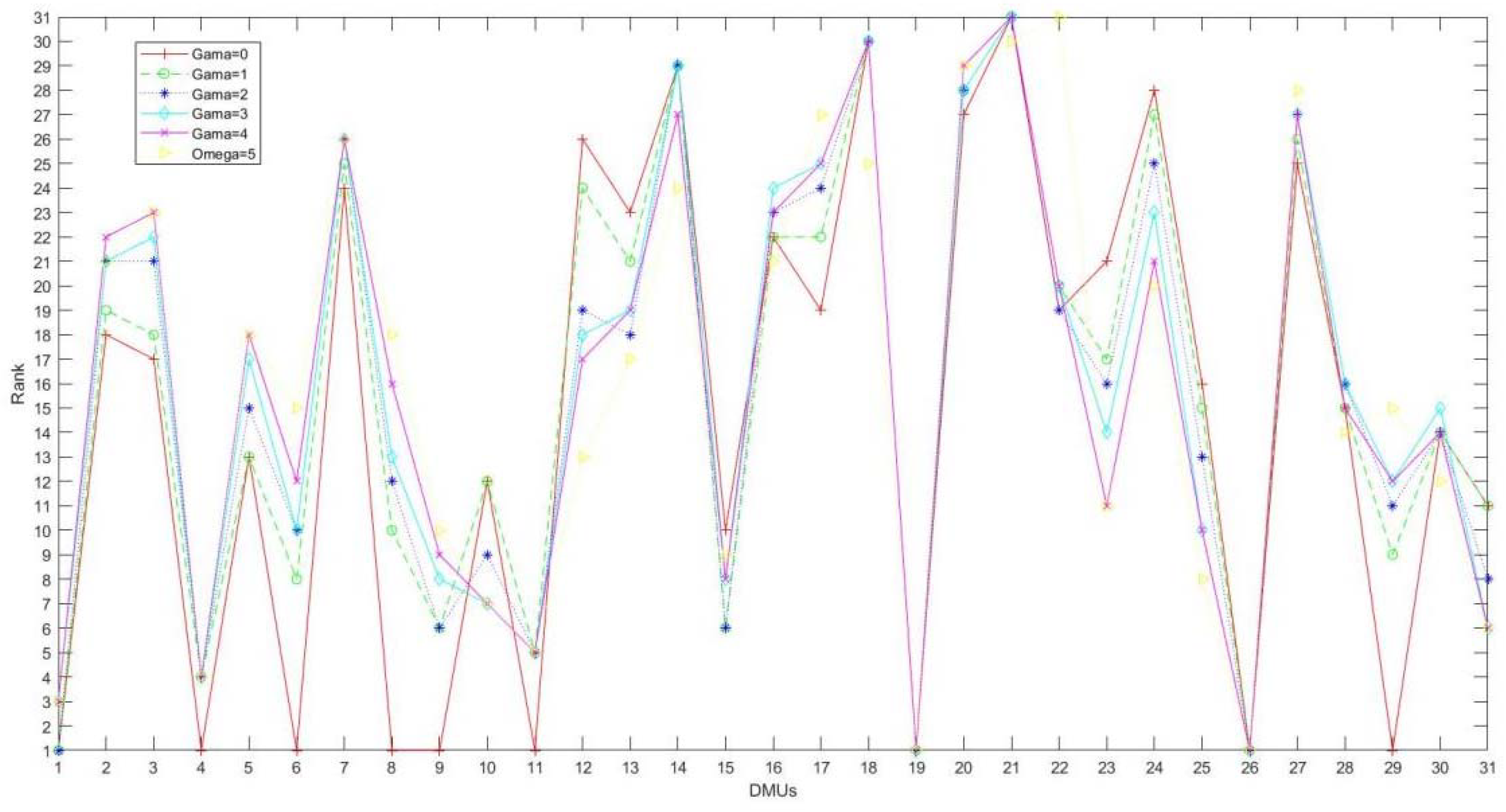
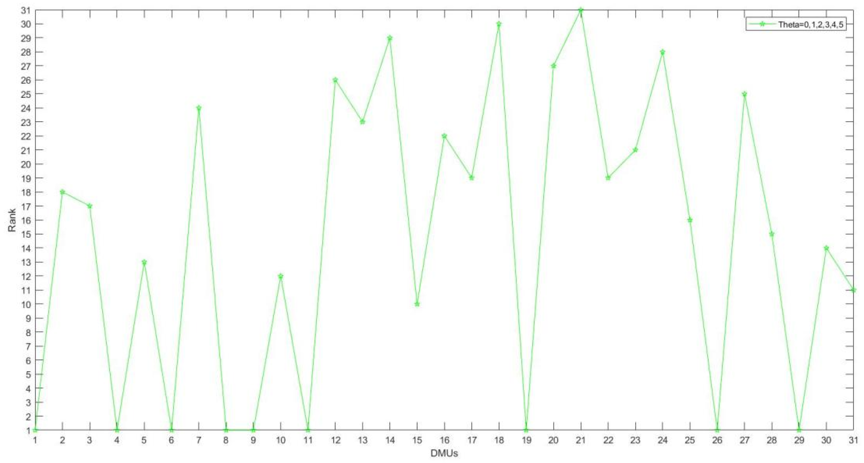
$\mathrm{\Phi },\mathrm{\Omega }$ and $\mathrm{\Gamma }$ in the robust DEA model are adjustable parameters to control the size level of an uncertain set, which represents the conservative degree of constraints. They not only describe the fluctuation of the value of the uncertain parameters in the geometry of a certain shape, but also reflect the uncertainty of the outputs. Figure 1 shows three curves of efficiency values varying with uncertainty parameters. With the increase of uncertainty parameters, the efficiency values based on different uncertain sets decrease at different speeds. Intuitively, the results of polyhedron uncertainty model and ellipsoid uncertainty model are better, the efficiency based on box uncertainty model performs the worst, and the results are far from those of the former two models. From the perspective of ranking, the results of the box uncertainty set and the ellipsoid uncertainty set show extremely strong stability. The results of the polyhedron uncertainty set show some fluctuation, but the fluctuation is acceptable. The results of rank are shown in Figure 2, Figure 3 and Figure 4, respectively. In general, the robust model with ellipsoidal uncertainty shows the highest efficiency and the strongest robustness.

4.5. Comparison between Interval DEA Model and Robust DEA Models

According to the previous subsection, we know that the robust DEA model based on ellipsoid uncertainty set performs the best. In this subsection, we compare the ellipsoid RDEA model with the interval DEA model, and the result are shown in Figure 5.

We compare the two models from two perspectives:

(1)

Is the result convenient to compare the efficiency of DMUs?

(2)

Is the result close to the real scenario?

According to the results shown in Figure 5, all the upper bounds of the IDEA model are 1. That is to say, all the DMUs can be judged to be effective under extremely favorable conditions. However, in the real world, the probability of this kind of situation is very low because it is difficult to make all units reach their best state. The lower bound of IDEA model ranges from 0.364 to 0.726, which seems to tell us that we can judge the efficiency ranking of DMUs with the same upper bound by comparing the lower bounds of DMUs. Yet this intuition is wrong, we have to know the distribution of efficiency value of each DMU, and this kind of information is often difficult to get in the real world. However, in the robust model, the final result is a certain number, and it is not necessary to determine the distribution of the value. The efficiency value of each DMU can be easily compared. From this point of view, the robust model performs better.

The result of the IDEA model is an interval. Its lower bound shows the lowest value that the DMU may take under the most unfavorable situation, while the upper bound shows the lowest value that the DMU may take under the most unfavorable situation. The IDEA model deals with uncertainty in the form of interval. However, once the interval is calculated, it is a value that cannot be adjusted. In the robust model, the uncertainty parameters describe the size of the uncertainty, we can adjust the size of the parameters according to the actual needs. The results are not only convenient to compare the efficiency of decision-making units, but also fit the real scenario, are more accurate, and provide important information for decision-makers. From the above analysis, a robust model is more suitable to solve our problem.

5. Data-Driven Robust DEA Models

In the Section 3, we assume that the output unit is uncertain because of the needs of the real situation. In the robust optimization method, there is not enough information and we also want to ensure the absolute robustness of the result, which leads to the result being too conservative. In the real situation, the tendency of macro policy of government can be expected approximately. At the same time, we can obtain some useful information from some historical data, rather than having no information available.

In the Section 5, contrary to the above, we assume that the observation sets of the output unit $P_{}$ can be obtained, where $P_{}=\{y_{r1},\dots ,y_{rM}\}$ and $y_{rq}\in R,q=1,\dots ,M$. In other words, $P_{}$ is the raw data that we can obtain. At the same time, let $y_r$ represent the average values of $\{y_{r1},\dots ,y_{rM}\}$, i.e., $\stackrel{\wedge }{y_r}=\frac{1}{M}{{\displaystyle {\sum }_{q\in M}y}}_{rq}$, where $[M]=\{1,\dots ,M\}$. Therefore, we need to find a decision variable that maximize the worst-case efficiency over all the costs in uncertainty set $Z$. This is the robust DEA problem:

$$\begin{array}{ll}\max & \{\underset{y_r\in {\rm Z}}{\min }{\displaystyle \sum _{r\in [s]}{u}_r{y}_r}\}\\ s.t.& {\displaystyle \sum _{i=1}^m{v}_i{x}_i}\le 0 \\ & {\displaystyle \sum _{\mathrm{r}=1}^{\mathrm{s}}{u}_r}{y}_{rj}-{\displaystyle \sum _{\mathrm{i}=1}^{\mathrm{m}}{v}_i}{x}_{ij}\le 0,{\forall }_j \\ & u_r,v_i\ge 0.\end{array}$$

(11)

In the next subsection, several methods for generating $Z$ will be introduced [35], where each set has a scaling parameter to control its size.

5.1. Box Uncertainty

We set $y_r^d={\min }_{q\in [M]}{y}_{rq},y_r^u={\max }_{q\in [M]}{y}_{rq}$, for any $\lambda \ge 0$, there is

$$Z_{Int}^U={\times }_{r\in [s]}[\stackrel{\wedge }{y_r}+\lambda (y_r^d-\stackrel{\wedge }{y_r}),\stackrel{\wedge }{y_r}+\lambda (y_r^a-\stackrel{\wedge }{y_r})],$$

where $\times$ is the Cartesian product and $[s]=\{1,\dots ,s\}$. It should be noticed that $\underset{y_r\in {\rm Z}}{\max }{\displaystyle \sum _{r\in [s]}{u}_r{y}_r}={\displaystyle \sum _{r\in [s]}{u}_r[\stackrel{\wedge }{y_{ro}}+\lambda (y_{ro}^a-\stackrel{\wedge }{y_{ro}})]}$.

Therefore, the robust problem obtained is

$$\begin{array}{ll}\min -& {\displaystyle \sum _{r\in [s]}{u}_r[\stackrel{\wedge }{y_{ro}}+\lambda (y_{ro}^a-\stackrel{\wedge }{y_{ro}})]}\\ s.t.& {\displaystyle \sum _{i=1}^m{v}_i{x}_i}\le 0 \\ & {\displaystyle \sum _{r\in [s]}{u}_r[\stackrel{\wedge }{y_{rj}}+\lambda (y_{rj}^a-\stackrel{\wedge }{y_{rj}})]}\le {\displaystyle \sum _{i=1}^m{v}_i{x}_{ij}},{\forall }_j \\ & u_r,v_r\ge 0.\\ \end{array}$$

(12)

Proof. 

For the objective function of (2), we just obtain its maximum value:

$$\underset{y_r\in {\rm Z}}{\max }{\displaystyle \sum _{r\in [s]}{u}_r{y}_r}={\displaystyle \sum _{r\in [s]}{u}_r[\stackrel{\wedge }{y_{ro}}+\lambda (y_{ro}^a-\stackrel{\wedge }{y_{ro}})]},$$

Then, it can be transformed to the equivalent form:

$$\min -{\displaystyle \sum _{r\in [s]}{u}_r[\widehat{y_{ro}}+\lambda (y_{ro}^a-\widehat{y_{ro}})]},$$

Similarly, the third inequality of (2) can be transformed to the following form:

$${\displaystyle \sum _{r\in [s]}{u}_r[\widehat{y_{rj}}+\lambda (y_{rj}^a-\widehat{y_{rj}})]}\le {\displaystyle \sum _{i=1}^m{v}_i{x}_{ij}},{\forall }_j.$$

Here, the size of box uncertainty set in decided by both uncertainty parameter and the observation sets, which is different from the box uncertainty set of Section 3.1. The proof of Section 5.2 and Section 5.3 is just similar to the proof above.□

5.2. Ellipsoidal Uncertainty

Ellipsoid uncertainty sets were derived from the observation that the iso-density locus of the multivariate normal distribution is an ellipse. Therefore, the maximum likelihood fit of a normal distribution $N(\mu ,\Sigma )$ of data point $\{y_{r1},\dots ,y_{rm}\}$ is given by $\mu =\stackrel{\wedge }{y_r},\Sigma =\frac{1}{M}{\displaystyle \sum _{q\in [M]}(y_{rq}-\mu )}{(y_{rq}-\mu )}^T$. We set an ellipsoid of the form $Z_{Elli}=\{y:{(y_r-\stackrel{\wedge }{y_r})}^T{\Sigma }^{-1}(y_r-\stackrel{\wedge }{y_r})\le r\}$ with the scaling parameter $\omega \ge 0$ and it is centered on $\stackrel{\wedge }{y_r}$. Following the similar proof of Section 5.1, the robust problem obtained is

$$\begin{array}{ll}\min -& {\displaystyle \sum _{r\in [s]}\stackrel{\wedge }{y_{ro}}{u}_r+\gamma }\\ s.t.& \omega \cdot u_r{}^T\Sigma u_r\le {\gamma }^2,\gamma \in [s]\\ & \omega \cdot u_r{}^T\Sigma u_r\le {\gamma }^2+{\displaystyle \sum _{i=1}^m{v}_i{x}_{ij},{\forall }_j}\\ & \hspace{1em}\hspace{1em}{\displaystyle \sum _{\mathrm{i}=1}^{\mathrm{m}}{v}_i{x}_i\le 1}\\ & \hspace{1em}\hspace{1em}{u}_r,v_i\ge 0.\end{array}$$

(13)

5.3. Polyhedron Uncertainty

A polyhedron defined using linear equations and inequalities is equivalent to a convex hull. We set $Z_{Poly}=\{y:\stackrel{\wedge }{y_r}+(y_r^a-\stackrel{\wedge }{y_r}){\alpha }_r,r\in [s],0\le \alpha \le 1,{\displaystyle \sum _{r\in [s]}{\alpha }_r\le \lambda }\}$ where the scaling parameter $\lambda$ controls the size of the set. Through the duality of the internal maximization problem, we arrive at the robust problem:

$$\begin{array}{ll}\min -& {\displaystyle \sum _{r\in [s]}\stackrel{\wedge }{y_r}{u}_r}+\lambda \gamma +||t|{|}_1\\ s.t& (y_{ro}^a-\stackrel{\wedge }{y_{ro}})u_r\le u+t_r,r\in [s]\\ & (y_{rj}^a-\stackrel{\wedge }{y_{rj}})u_r\le u+t_r+{\displaystyle \sum _{i=1}^m{x}_{ij}{v}_i},{\forall }_j \\ & \hspace{1em}\hspace{1em}{\displaystyle \sum _{i=1}^m{v}_i{x}_i}\le 1\\ & \hspace{1em}\hspace{1em}{u}_r,v_i\ge 0.\end{array}$$

(14)

5.4. Numerical Analysis

It is obvious that the scaling parameters will affect the size of each uncertainty set. Here, we just follow the analysis of Section 4, comparing the trends of three proposed uncertainty sets under the same scaling parameters. Scaling parameters here are set from 1 to 5 with a step of 1. In this way, we can clearly see the gradual change of efficiency value.

When the uncertainty set is an interval set, the RDEA efficiency values of 31 DMUs are shown in

Table 6. Data-driven robust DEA efficiency based on interval set.

Province	RDEA Efficiency					Rank
	$\lambda$ = 1	$\lambda$ = 2	$\lambda$ = 3	$\lambda$ = 4	$\lambda$ = 5	R
Beijing	0.942	0.869	0.804	0.738	0.682	01
Tianjin	0.863	0.795	0.733	0.675	0.621	18
Hebei	0.875	0.797	0.735	0.675	0.617	14
Shanxi	0.939	0.866	0.802	0.736	0.679	05
Neimenggu	0.877	0.799	0.737	0.676	0.619	13
Liaoning	0.899	0.823	0.759	0.695	0.639	10
Jilin	0.804	0.738	0.679	0.621	0.570	25
Heilongjiang	0.881	0.803	0.741	0.679	0.623	12
Shanghai	0.942	0.869	0.804	0.738	0.682	01
Jiangsu	0.942	0.869	0.804	0.738	0.682	01
Zhejiang	0.882	0.805	0.742	0.681	0.625	11
Anhui	0.802	0.736	0.677	0.620	0.568	26
Fujian	0.828	0.761	0.701	0.644	0.592	23
Jiangxi	0.792	0.726	0.668	0.611	0.559	27
Shandong	0.939	0.866	0.802	0.736	0.679	05
Henan	0.823	0.757	0.697	0.639	0.588	24
Hubei	0.862	0.794	0.732	0.674	0.619	19
Hunan	0.744	0.679	0.622	0.566	0.515	31
Guangdong	0.941	0.868	0.803	0.737	0.681	04
Guangxi	0.784	0.718	0.660	0.604	0.552	28
Hainan	0.852	0.784	0.723	0.665	0.613	21
Chongqing	0.856	0.788	0.727	0.669	0.614	20
Sichuan	0.834	0.766	0.706	0.649	0.597	22
Guizhou	0.774	0.708	0.651	0.595	0.544	30
Yunnan	0.866	0.799	0.737	0.679	0.625	17
Xizang	0.917	0.841	0.777	0.711	0.655	07
Shanxi	0.782	0.716	0.658	0.602	0.551	29
Gansu	0.872	0.794	0.732	0.673	0.615	15
Qinghai	0.917	0.841	0.777	0.711	0.655	07
Ningxia	0.872	0.794	0.732	0.673	0.615	15
Xinjiang	0.901	0.825	0.762	0.697	0.642	09
Mean	0.865	0.793	0.732	0.671	0.617

. When the uncertainty parameter $\lambda$ equals 1, the maximum value of the efficiency of endowment insurance system in 31 provinces is 0.942, the minimum value is 0.744. Compared with the Robust DEA model, the result has a larger range. The efficiency rank of some provinces has changed greatly under uncertain circumstances. For example, in the robust DEA model, the rank of Hainan is the last one, but it soars up to 21st in a data-driven robust DEA model. When the uncertainty set is an ellipsoidal set, the RDEA efficiency values of 31 DMUs are shown in

Table 7. Data-driven robust DEA efficiency based on ellipsoidal set.

Province	RDEA Efficiency					Rank
	$\omega$ = 1	$\omega$ = 2	$\mathrm{\omega }$ = 3	$\mathrm{\omega }$ = 4	$\mathrm{\omega }$ = 5	R
Beijing	0.965	0.890	0.823	0.756	0.698	01
Tianjin	0.884	0.814	0.751	0.691	0.636	18
Hebei	0.896	0.816	0.753	0.691	0.632	14
Shanxi	0.962	0.887	0.821	0.754	0.695	05
Neimenggu	0.898	0.818	0.755	0.692	0.634	13
Liaoning	0.921	0.843	0.777	0.712	0.654	10
Jilin	0.823	0.756	0.695	0.636	0.584	25
Heilongjiang	0.902	0.822	0.759	0.695	0.638	12
Shanghai	0.965	0.890	0.823	0.756	0.698	01
Jiangsu	0.965	0.890	0.823	0.756	0.698	01
Zhejiang	0.903	0.824	0.760	0.697	0.640	11
Anhui	0.821	0.754	0.693	0.635	0.582	26
Fujian	0.848	0.779	0.718	0.659	0.606	23
Jiangxi	0.811	0.743	0.684	0.626	0.572	27
Shandong	0.962	0.887	0.821	0.754	0.695	05
Henan	0.843	0.775	0.714	0.654	0.602	24
Hubei	0.883	0.813	0.750	0.690	0.634	19
Hunan	0.762	0.695	0.637	0.580	0.527	31
Guangdong	0.964	0.889	0.822	0.755	0.697	04
Guangxi	0.803	0.735	0.676	0.618	0.565	28
Hainan	0.872	0.803	0.740	0.681	0.628	21
Chongqing	0.877	0.807	0.744	0.685	0.629	20
Sichuan	0.854	0.784	0.723	0.665	0.611	22
Guizhou	0.793	0.725	0.667	0.609	0.557	30
Yunnan	0.887	0.818	0.755	0.695	0.640	17
Xizang	0.939	0.861	0.796	0.728	0.671	07
Shanxi	0.801	0.733	0.674	0.616	0.564	29
Gansu	0.893	0.813	0.750	0.689	0.630	15
Qinghai	0.939	0.861	0.796	0.728	0.671	07
Ningxia	0.893	0.813	0.750	0.689	0.630	15
Xinjiang	0.923	0.845	0.780	0.714	0.657	09
Mean	0.886	0.812	0.749	0.687	0.631

. Similar to the interval uncertainty sets of data-driven DEA model, the result shows a larger range and a more stable decreasing with the increasing of the uncertainty level.

While the uncertainty set turns out to be a polyhedron set, the rank is quite different with that in robust DEA model. From the

Table 8. Data-driven robust DEA efficiency based on polyhedron set.

Province	RDEA Efficiency (Rank)
	$\mathrm{\Gamma }$ = 1	$\mathrm{\Gamma }$ = 2	$\mathrm{\Gamma }$ = 3	$\mathrm{\Gamma }$ = 4	$\mathrm{\Gamma }$ = 5
Beijing	0.957 (01)	0.884 (01)	0.816 (01)	0.754 (01)	0.696 (01)
Tianjin	0.881 (18)	0.807 (18)	0.745 (18)	0.696 (18)	0.643 (18)
Hebei	0.907 (14)	0.833 (14)	0.769 (14)	0.710 (14)	0.656 (14)
Shanxi	0.946 (07)	0.872 (07)	0.805 (07)	0.656 (07)	0.606 (07)
Neimenggu	0.918 (12)	0.844 (12)	0.779 (12)	0.720 (12)	0.664 (12)
Liaoning	0.924 (11)	0.850 (11)	0.784 (11)	0.664 (11)	0.614 (11)
Jilin	0.823 (25)	0.755 (25)	0.697 (25)	0.644 (25)	0.594 (25)
Heilongjiang	0.914 (13)	0.844 (12)	0.779 (12)	0.594 (12)	0.549 (12)
Shanghai	0.951 (05)	0.876 (05)	0.809 (05)	0.747 (05)	0.690 (05)
Jiangsu	0.954 (03)	0.880 (03)	0.813 (03)	0.690 (03)	0.637 (03)
Zhejiang	0.929 (10)	0.854 (10)	0.789 (10)	0.728 (10)	0.672 (10)
Anhui	0.821 (26)	0.753 (26)	0.695 (26)	0.672 (26)	0.621 (26)
Fujian	0.848 (24)	0.777 (24)	0.717 (24)	0.662 (24)	0.612 (24)
Jiangxi	0.815 (27)	0.747 (27)	0.690 (27)	0.612 (27)	0.565 (27)
Shandong	0.948 (06)	0.874 (06)	0.807 (06)	0.745 (06)	0.688 (06)
Henan	0.851 (23)	0.780 (23)	0.714 (23)	0.688 (23)	0.635 (23)
Hubei	0.875 (20)	0.802 (20)	0.720 (20)	0.684 (20)	0.631 (20)
Hunan	0.749 (31)	0.672 (31)	0.684 (31)	0.631 (31)	0.583 (31)
Guangdong	0.954 (03)	0.879 (04)	0.812 (04)	0.749 (04)	0.692 (04)
Guangxi	0.801 (28)	0.722 (28)	0.749 (28)	0.692 (28)	0.639 (28)
Hainan	0.872 (21)	0.799 (21)	0.738 (21)	0.681 (21)	0.629 (21)
Chongqing	0.877 (19)	0.804 (19)	0.681 (19)	0.629 (19)	0.581 (19)
Sichuan	0.858 (22)	0.786 (22)	0.726 (22)	0.670 (22)	0.619 (22)
Guizhou	0.781 (30)	0.703 (30)	0.670 (30)	0.619 (30)	0.571 (30)
Yunnan	0.893 (17)	0.819 (17)	0.756 (17)	0.698 (17)	0.645 (17)
Xizang	0.946 (07)	0.872 (07)	0.698 (07)	0.645 (07)	0.595 (07)
Shanxi	0.795 (29)	0.716 (29)	0.661 (29)	0.610 (29)	0.564 (29)
Gansu	0.907 (14)	0.833 (14)	0.610 (14)	0.564 (14)	0.520 (14)
Qinghai	0.957 (01)	0.883 (02)	0.815 (02)	0.753 (02)	0.695 (02)
Ningxia	0.907 (14)	0.832 (16)	0.753 (16)	0.695 (16)	0.642 (16)
Xinjiang	0.941 (09)	0.866 (09)	0.800 (09)	0.738 (09)	0.682 (09)
Mean	0.887	0.813	0.744	0.678	0.626

, we can explicitly see that the rank is gradually in a fairly stable state when the uncertainty parameter is greater than 2.

From the analysis above, we can obtain the following conclusion:

(1)

In a data-driven robust DEA model, among three uncertainty sets, the ellipsoidal set shows the strongest robustness which is similar to the robust DEA model.

(2)

Compared with robust DEA model, the data-driven robust DEA model shows better performance. All three uncertainty sets have greater efficiency than the former. It is worth mentioning that the rank is gradually in a fairly stable state when the uncertainty parameter greater than 2. The reason for these two phenomena is also easy to find. In data-driven methods, more information is provided, so we can describe the uncertainty more accurately, which leads to the more satisfactory result.

5.5. Managerial Insights

The only drawback of the robust model is that it may lead to over conservative results. For this reason, we use data-driven method to solve it. According to the results shown in Table 2, the lowest efficiency of endowment insurance system among 31 provinces is 0.857 (Hainan Province). The endowment insurance system efficiency value of 28 provinces is higher than 0.9, which means that China’s endowment insurance system is generally in good condition. On the other hand, as shown in Figure 5, there is little difference in the efficiency of endowment insurance among 31 provinces, which means that the difference between regions is not significant. From the results shown in Figure 1, with the increase of uncertainty, the efficiency of endowment insurance system in China’s provinces shows a downward trend.

At the same time, the increase of population aging and the improvement of life expectancy are a fixed trend in the next 30 years, which leads to the increase of endowment insurance expenditure. The Chinese government must increase the financial expenditure on endowment insurance to resolve this grim situation. For some provinces with low efficiency, such as Shanxi, Hunan, Hainan, the government should give priority to providing subsidies to promote fair distribution. What is more, local governments should pay more attention to the development of the endowment insurance system, and pay attention to the differences in the operation of the endowment insurance system in different regions. To improve the operation efficiency of endowment insurance, the government of underdeveloped regions can consider learning from the advanced systems and experience of other areas and reasonably guide the input and output of resources.

6. Conclusions

In this research, robust optimization is applied to a DEA model to deal with data uncertainty. The proposed robust model considers three kinds of uncertainty sets: ellipsoidal uncertainty set, box uncertainty set, polyhedron uncertainty set. At the same time, data-driven robust method was applied to solve its inherent defects, which is over-conservative. The results show that the polyhedron robust model has the worst result, while the ellipsoidal uncertain model has the strongest robustness and the most favorable efficiency. From the analysis of the results, we can describe the uncertainty of market environment by adjusting the size of uncertainty parameters, so as to meet our actual needs. The proposed model was applied to the endowment insurance system of various provinces in China, and it was found that China’s endowment insurance system generally operates at a high level and the difference between regions is not significant. In the future, the government should increase financial support for endowment insurance, especially in underdeveloped regions. The government of relatively underdeveloped regions should learn from developed regions to improve the operation efficiency of local pension insurance system.

References

1. National Bureau of Statistics. Bulletin of the Seventh National Census. 2020. Available online: http://www.stats.gov.cn (accessed on 8 August 2022).
2. Cai, F. Supply- and Demand-side Impacts of Aging on China’s Economic Growth. Econ. Perspect. 2021, 1, 27–34. [Google Scholar]
3. Samuelson, P.A. The Pure Theory of Public Expenditure. Rev. Econ. Stat. 1954, 36, 387–389. [Google Scholar] [CrossRef]
4. Diamond, P. National Debt in a Neoclassical Growth Model. Am. Econ. Rev. 1965, 55, 1126–1150. [Google Scholar]
5. Aaron, H.J. The Social Insurance Paradox. Can. J. Econ. Political Sci. 1966, 33, 371–374. [Google Scholar] [CrossRef]
6. Zhang, X.; Liu, X.; Wang, Y.; Zhou, L.; Cheng, X. Sustainable Development of China’s Maternity Insurance System in the Context of Population Policy Changes: Using a Grounded Theory Approach. Sustainability 2022, 14, 2138. [Google Scholar] [CrossRef]
7. Xue, Z.; Ma, Z. Performance Evaluation of China’s Basic Pension Insurance Based on a Three-Stage Superefficient SBM-DEA Model. Discret. Dyn. Nat. Soc. 2022, 2022, 2429927. [Google Scholar] [CrossRef]
8. Charnes, A.; Cooper, W.W. Measuring the efficiency of decision making units. Eur. J. Oper. Res. 1978, 2, 429–444. [Google Scholar] [CrossRef]
9. Banker, R.D.; Charnes, A.; Cooper, W.W. Some models for estimating technical and scale inefficiencies in data envelopment analysis. Manag. Sci. 1984, 30, 1078–1092. [Google Scholar] [CrossRef]
10. Chen, Z.F. Chinese bank efficiency during the global financial crisis: A combined approach using satisficing DEA and Support Vector Machines. N. Am. J. Econ. Financ. 2018, 43, 71–86. [Google Scholar] [CrossRef]
11. Shaddady, A.; Moore, T. Investigation of the effects of financial regulation and supervision on bank stability: The application of CAMELS-DEA to quantile regressions. J. Int. Financ. Mark. Inst. Money 2019, 58, 96–116. [Google Scholar] [CrossRef]
12. Asmild, M.; Zhu, M.Y. Controlling for the use of extreme weights in bank efficiency assessments during the financial crisis. Eur. J. Oper. Res. 2016, 251, 999–1015. [Google Scholar] [CrossRef]
13. Geng, Z.Q.; Zeng, R.F. Energy efficiency evaluation and energy saving based on DEA integrated affinity propagation clustering: Case study of complex Petrochemical industries. Energy 2016, 179, 863–875. [Google Scholar] [CrossRef]
14. Moon, H.; Min, D. Assessing energy efficiency and the related policy implicatio- ns for energy-intensive firms in Korea: DEA approach. Energy 2017, 133, 23–34. [Google Scholar] [CrossRef]
15. Meng, F.Y.; Su, B. Measuring China’s regional energy and carbon emission efficiency with DEA models: A survey. Appl. Energy 2016, 183, 1–21. [Google Scholar] [CrossRef]
16. Oukil, A.; El-Bouri, A.; Emrouznejad, A. Energy-aware job scheduling in a multi-objective production environment—An integrated DEA-OWA model. Comput. Ind. Eng. 2022, 168, 108065. [Google Scholar] [CrossRef]
17. Aparicio, J.; Cordero, J.M. Using non-radial DEA to assess school efficiency in a cross-country perspective: An empirical analysis of OECD countries. Omega 2018, 79, 9–20. [Google Scholar] [CrossRef]
18. Huang, M.; Xia, T.; Chen, Z.; Pan, E.; Xi, L. A DEA integrated grey factor analysis approach for efficiency evaluation and ranking in uncertain systems. Comput. Ind. Eng. 2021, 162, 107681. [Google Scholar] [CrossRef]
19. Nyamuhirwa, D.M.A.; Awotide, B.A.; Kusinza, D.B.; Bishikwabo, V.K.; Mignouna, J.; Bamba, Z.; Dontsop Nguezet, P.M. A Comparative Analysis of Technical Efficiency and Profitability of Agribusiness and Non-Agribusiness Enterprises in Eastern DRC. Sustainability 2022, 14, 8384. [Google Scholar] [CrossRef]
20. Wang, Q.; Chen, Y.; Guan, H.; Lyulyov, O.; Pimonenko, T. Technological Innovation Efficiency in China: Dynamic Evaluation and Driving Factors. Sustainability 2022, 14, 8321. [Google Scholar] [CrossRef]
21. Pendharkar, P.C.; Rodger, J.A. Quantitative software project management with mixed data: A comparison of radial, nonradial, and ensemble data envelopment analysis models. J. Softw. Evol. Process 2021, 33, e2348. [Google Scholar] [CrossRef]
22. Álvarez, I.; Barbero, J.; Zofío, J.L. A Data Envelopment Analysis Toolbox for MATLAB (No. 2016/03). Ph.D. Thesis, Universidad Autónoma de Madrid (Spain), Department of Economic Analysis (Economic Theory and Economic History), Madrid, Spain, 2016. [Google Scholar]
23. Andreu, L.; Sarto, J.L.; Vicente, L. Efficiency of the strategic style of pension funds: An application of the variants of the slacks-based measure in DEA. J. Oper. Res. Soc. 2014, 65, 1886–1895. [Google Scholar] [CrossRef]
24. Hu, Y.M.; Li, T. Evaluation of the Efficiency of Basic Pension Insurance System Operation of Urban and Rural Residents. J. Agro-For. Econ. Manag. 2019, 18, 742–751. [Google Scholar]
25. Soyster, A.L. Convex programming with set-inclusive constraints and applications to inexact linear programming. Oper. Res. 1973, 21, 1154–1157. [Google Scholar] [CrossRef]
26. El Ghaoui, L.; Lebret, H. Robust solutions to least-square problems to uncertain data matrices. SIAM J. Matrix Anal. Appl. 1997, 18, 1035–1064. [Google Scholar] [CrossRef]
27. Ben-Tal, A.; Nemirovski, A. Robust Convex Optimization. Math. Oper. Res. 1998, 23, 769–805. [Google Scholar] [CrossRef]
28. Ben-Tal, A.; Nemirovski, A. Robust solutions of uncertain liner programs. Oper. Res. Lett. 1999, 25, 1–13. [Google Scholar] [CrossRef]
29. Ben-Tal, A.; Nemirovski, A. Robust solutions of uncertain liner programming contained data. Math. Program. 2000, 88, 411–424. [Google Scholar] [CrossRef]
30. Bertsimas, D.; Sim, M. Robust discrete optimization and network flows. Math. Program. 2003, 98, 49–71. [Google Scholar] [CrossRef]
31. Bertsimas, D.; Sim, M. The price of robustness. Oper. Res. 2004, 52, 35–53. [Google Scholar] [CrossRef]
32. Bertsimas, D.; Sim, M. Tractable approximations to robust conic optimization problems. Math. Program. 2006, 107, 5–36. [Google Scholar] [CrossRef]
33. Bertsimas, D.; Pachamanova, D.; Sim, M. Robust linear optimization under general norms. Oper. Res. Lett. 2004, 32, 510–516. [Google Scholar] [CrossRef]
34. Sadjadi, S.J.; Omrani, H. Data envelopment analysis with uncertain data: An application for Iranian electricity distribution companies. Energy Policy 2008, 36, 4247–4254. [Google Scholar] [CrossRef]
35. Kazemia, I.; Haji, H.A. A robust DEA model for measuring the relative efficiency of Iranian high schools. Manag. Sci. Lett. 2011, 1, 389–404. [Google Scholar]
36. Bertsimas, D.; Gupta, V.; Kallus, N. Data-driven robust optimization. Math. Program. 2018, 167, 235–292. [Google Scholar] [CrossRef]
37. Chassein, A.; Dokka, T.; Goerigk, M. Algorithms and uncertainty sets for data-driven robust shortest path problems. Eur. J. Oper. Res. 2019, 274, 671–686. [Google Scholar] [CrossRef]
38. Ben-Tal, A.; El Ghaoui, L.; Nemirovski, A. Robust Optimization; Princeton University Press: Princeton, NJ, USA, 2009. [Google Scholar]
39. National Bureau of Statistics. Endowment Insurance for Urban Employees by Region 2019. 2020. Available online: http://www.stats.gov.cn/tjsj/ndsj/2020/indexch.htm (accessed on 8 August 2022).
Figure 1. Comparison between different uncertainty sets.
Sustainability 14 09954 g001
Figure 2. The rank of 31 DMUs in different uncertainty levels (box uncertainty).
Sustainability 14 09954 g002
Figure 3. The rank of 31 DMUs in different uncertainty levels (ellipsoid uncertainty).
Sustainability 14 09954 g003
Figure 4. The rank of 31 DMUs in different uncertainty levels (polyhedron uncertainty).
Sustainability 14 09954 g004
Figure 5. Efficiency of 31 DMUs based on different models.
Sustainability 14 09954 g005