Climate Smart Pest Management

Abstract

This study examines the role of weather and pest infestation forecasts in agricultural pest management, taking into account potential correlation between weather and pest population prediction errors. First, we analytically illustrate the role of the correlation between weather and pest infestation forecast errors in pest management using a stochastic optimal control framework. Next, using stochastic dynamic programming, we empirically simulate optimal pest management trajectory within a growing season, taking into account correlation between weather and pest population prediction errors. We used lentil production in the Palouse area of northern Idaho and eastern Washington as a case study, where pesticide use was restricted due to environmental or health reasons. We showed that the benefit of applying pesticides later in the growing season can outweigh benefits of early application when pesticide use is restricted due to environmental or health regulations. The value of information is close to $9 per acre, approximately 8% of the expected net returns per acre, and close to $12 per acre ($106–$94), or approximately 13% of the expected net returns per acre for the baseline versus the climate change scenarios, respectively.

1. Introduction

One of the consequences of projected climatic changes is a potential increase in frequency and intensity of regional agricultural pest outbreaks [1,2,3]. Consequently, pest management is to remain a high priority for the industry, as well as public agencies involved in regulatory aspects of agricultural pest management [4]. The industry continues to search for opportunities to minimize costs associated with pest invasions and control. On the other hand, the regulators seek to balance pest management objectives with potential externalities of pest management pertaining to environmental quality and health [5]. This requires a new way of analytical thinking, pest management practice, and up-to-date regulation, which we call climate smart pest management. The main goal of this article is to provide a framework for analyzing the dynamics of pest management activities given uncertain weather conditions and pest population throughout the growing season. Our objective is to evaluate optimal pest management dynamics during the growing season when deviations of weather and pest populations from respective expected values can be correlated.

Economists have studied pest management using specifications which explicitly include damage (or damage control) functions in conjunction with production functions [6,7,8,9] The advantage of such formulations is that the modeler can separate the effects of direct production inputs from the effects of pest control inputs. The effects of weather conditions on agricultural productivity in general are also established [10,11,12,13]. We followed the literature on the effects of weather and climate on agricultural productivity and the literature on damage function specification in pest management [10,14,15] to study the influence of climate conditions on pest management specifically.

In the context of stochastic weather and pest infestation dynamics, the framework for examination of optimal pest management activities throughout the growing season requires explicit consideration of the following assumptions and elements: (a). Dynamic model where farmers make pesticide use decision throughout the growing season (Adaptation to climate change could also involve switching to a different crop, which is not the focus of this paper. Here, we assume that crop planting decisions have been made in the beginning of the growing season); (b). Pest population evolves over time through both pest infestations and pest outbreaks; (c). Pest populations are stochastic due to potential repeated infestations and stochastic growth; (d) Weather conditions change over time within a growing season and are also stochastic in nature; (e). Climate change may bring higher temperature and higher volatility in weather conditions, the stochastic processes of pest population and weather conditions may be correlated; (f) Pesticide use is restricted due to environmental or health reasons.

The current literature has approached several aspects of the factors above: (a) and (b) are extensively studied [16,17,18,19] through dynamic models of pest population growth over time. Dynamic models explicitly capture not only the benefits of removing the pests in the current period but also the discounted sum of benefits of avoiding the damages that would have been caused by the offsprings of pests removed in the current period. Hertzler [20] suggests that diffusion process-based stochastic dynamic models and Ito’s calculus can be used for economic studies of pest control in agricultural production. Since then, (a–c) has been studied by Richards et al. and Saphores et al. (see [21,22,23,24] for details). Articles such as [25,26] discuss stochastic dynamic programming problems with more than one source of randomness, which can be redeemed as a general formulation that could discuss the implications of (a) and (e). However, to the best of our knowledge, no studies have examined dynamic invasive species management in a comprehensive system that captures all of the features from (a) to (f).

In this article, we revisit the issue of optimal agricultural pest management and illustrate the effect of stochastic weather and pest outbreak dynamics on optimal pesticide use throughout the growing season. We show that deviations of pest populations and weather from respective expected trajectories during the growing season can be used to to improve the timing and profitability of pesticide use. In particular, if deviations of pest populations and weather from the respective expected paths are known to be correlated and this correlation is taken into account, then the timing of pesticide application can be improved relative to the application schedule where the correlation is disregarded. We also provide an empirical illustration based on the formulations in the preceding section. The empirical model is presented for the case of lentil production in the Pacific Northwest where outbreaks of pea aphids frequently threaten the profitability of the lentil industry [27]. There are four main contributions out of this article. First, we discuss pest management in a stochastic and dynamic setting with two sources of randomness and provide a closed form solution to the problem. Second, the framework proposed in this paper can be applied in numerous other contexts where forecasts of two stochastic factors can be used to improve natural resource management. For example, the framework can be used in such contexts as invasive species, wild fire, and water resource management. Third, in cases where correlation between deviations of pest infestation and weather from respective expected values is non-zero, improved pest management can lead to a more cost efficient use of pesticides. Fourth, we extend the previous literature, which a provides rationale for application of pesticides early in the growing season. We demonstrate that in cases where pesticide use is restricted due to environmental or health reasons, the benefit of application later in the growing season can outweigh the benefit of applying early.

2. Materials and Methods

The framework is based on maximizing terminal value of production within a growing season, which includes profit losses due to pest inflicted damages as well as costs of control efforts. Crop biomass growth in this formulation explicitly depends on stochastic pest invasions and stochastic weather conditions.

2.1. The General Conceptual Framework

We use a non-negative index $\theta \left(t\right)$ to denote weather conditions (For a discussion of degree day accumulation, see [16,28]). The weather index is assumed to follow a diffusion process [29]:

$$\begin{array}{c}\hfill d\theta ={\mu }^{\theta }\left(\theta ,t\right)dt+{\sigma }^{\theta }\left(\theta ,t\right)d\tilde{\theta },\end{array}$$

(1)

where ${\mu }^{\theta }$ and ${\sigma }^{\theta }$ denote expected changes in the weather index and corresponding standard deviation over time, respectively. $\tilde{\theta }$ is the standard Wiener process, i.e., $\tilde{\theta }\sim N(0,t)$ with $var\left(d\tilde{\theta }\right)=dt$. Consequently, the standard deviation of $\tilde{\theta }$ is expanding with constant increments over time. At any time t, ${\mu }^{\theta }$ can be interpreted as the predictable or expected rate of change of the weather index with standard deviation ${\sigma }^{\theta }$. Both ${\mu }^{\theta }$ and ${\sigma }^{\theta }$ vary with time as well as weather conditions.

Pest population is formulated as:

$$\begin{array}{c}\hfill A\left(t\right)=A\left(u\left(t\right),\theta \left(t\right),t,\tilde{A}\right),\end{array}$$

(2)

where $u\left(t\right)$ denotes pest control activities like pesticide use, $\tilde{A}$ represents another Wiener process (i.e., $\tilde{A}\sim N(0,t)$ with $var\left(d\tilde{A}\right)=dt$), which can be attributed to all other uncontrolled factors that affect pest population besides weather, pest management activities, and time. A is assumed to be twice differentiable in all of its arguments. Applying Ito’s Lemma [20,30], and substituting (1), we have (We use subscripts to denote derivatives throughout the current and the following sections) (see Appendix A):

$$\begin{array}{c}\hfill dA=\left(A_t+A_{\theta }{\mu }^{\theta }+\frac{1}{2}{A}_{\theta \theta }{\left({\sigma }^{\theta }\right)}^2+\frac{1}{2}{A}_{\tilde{A}\tilde{A}}+A_{\theta \tilde{A}}{\rho }^{\tilde{\theta }\tilde{A}}{\sigma }^{\theta }\right)dt+A_{\theta }{\sigma }^{\theta }d\tilde{\theta }+A_{\tilde{A}}d\tilde{A}.\end{array}$$

(3)

Equation (3) explicitly includes an interaction between stochastic weather index and stochastic pest population. Unexplained variability in weather and unexplained variability in pest population are correlated, via $d\tilde{\theta }d\tilde{A}={\rho }^{\tilde{\theta }\tilde{A}}dt$ [30], where ${\rho }^{\tilde{\theta }\tilde{A}}$ denotes the correlation between $d\tilde{\theta }$ and $d\tilde{A}$. Non-zero ${\rho }^{\tilde{\theta }\tilde{A}}$ implies that differences in deviations from expected changes of weather index can be correlated with differences in corresponding unexplained deviations of pest dynamics.

Let ${\mu }^A\left(u,A,\theta ,t\right)\equiv A_t+A_{\theta }{\mu }^{\theta }+\frac{1}{2}{A}_{\theta \theta }{\left({\sigma }^{\theta }\right)}^2+\frac{1}{2}{A}_{\tilde{A}\tilde{A}}+A_{\theta \tilde{A}}{\rho }^{\tilde{\theta }\tilde{A}}{\sigma }^{\theta }$ denote the deterministic growth rate of pest population which includes second order components from Ito’s Lemma but does not include the stochastic elements. We can rewrite the pest population dynamics equation as:

$$\begin{array}{c}\hfill dA={\mu }^A\left(u,A,\theta ,t\right)dt+A_{\theta }{\sigma }^{\theta }\left(\theta ,t\right)d\tilde{\theta }+A_{\tilde{A}}d\tilde{A}.\end{array}$$

(4)

Equation (4) shows that A is also following a diffusion process. Specifications based on similar diffusion processes can be found in prior studies [23,31]. However, rather than having a single source of randomness, here the change in pest population has two sources of randomness—one associated with weather ($\tilde{\theta }$) and the other associated with remaining factors which can affect pest population dynamics ($\tilde{A}$). We assume that ${\mu }^A$ is decreasing in the pesticide use, u. Keeping in mind that $d\tilde{\theta }d\tilde{\theta }=dt$ and $d\tilde{A}d\tilde{A}=dt$, the variance of $dA$ is:

$$\begin{array}{c}Var\left(dA\right)=Var(A_{\theta }{\sigma }^{\theta }d\tilde{\theta }+A_{\tilde{A}}d\tilde{A})\hfill \\ \hfill \hspace{1em}\hspace{1em}\hspace{1em}\hspace{1em}\hspace{1em}\hspace{1em}\hspace{1em}\hspace{1em}\hspace{1em}\hspace{1em}\hspace{1em}\hspace{1em}\hspace{1em}={\left(A_{\theta }{\sigma }^{\theta }\right)}^{2}dt+{\left(A_{\tilde{A}}\right)}^{2}dt+2A_{\theta }{A}_{\tilde{A}}{\rho }^{\tilde{\theta }\tilde{A}}{\sigma }^{\theta }dt\equiv {\left({\sigma }^A\right)}^{2}dt.\end{array}$$

(5)

Next, we formulate losses in crop biomass growth as a function of stochastic weather and pest population dynamics.

$$\begin{array}{c}\hfill L\left(t\right)=L\left(A\left(u\left(t\right),\theta \left(t\right),t,\tilde{A}\right),\theta (t,\tilde{\theta }),t\right)\end{array}$$

(6)

We assume that the loss in crop biomass growth, L, is twice differentiable with respect to all of its arguments and is increasing in A (Notice that the weather index ($\theta$) is an exogenous variable. It affects the state variables, pest (A) and loss (L) dynamics, but is not a function of control variable (u)). Using Ito’s lemma and Equations (1) and (4), the dynamics of losses in crop biomass growth can be expressed as (see Appendix B):

$$\begin{array}{c}\hfill dL={\mu }^L\left(u,A,L,\theta ,t\right)dt+\left(L_{\theta }{\sigma }^{\theta }\left(\theta ,t\right)+L_A{A}_{{}^{\theta }}{\sigma }^{\theta }\left(\theta ,t\right)\right)d\tilde{\theta }+L_A{A}_{\tilde{A}}d\tilde{A},\end{array}$$

(7)

where ${\mu }^L=\left(L_t+L_{\theta }{\mu }^{\theta }+L_A{\mu }^A+\frac{1}{2}{L}_{\theta \theta }{\left({\sigma }^{\theta }\right)}^2+\frac{1}{2}{L}_{AA}{\left({\sigma }^A\right)}^2+{L_{\theta }}_A{\rho }^{\tilde{\theta }\tilde{A}}{\sigma }^{\theta }{\sigma }^A\right)$, which denotes the expected crop biomass growth loss rate as a function of weather index and pest population and is assumed to be decreasing in u. Variance of $dL$ is the variance of the sum of two stochastic components (last two terms of Equation (7)) and can be expressed as follows, keeping in mind that Wiener process specification implies $d\tilde{\theta }d\tilde{\theta }=dt$, $d\tilde{A}d\tilde{A}=dt$ and $d\tilde{\theta }d\tilde{A}={\rho }^{\tilde{\theta }\tilde{A}}dt$:

$$\begin{array}{c}{\left({\sigma }^L\right)}^{2}dt={\left(L_{\theta }{\sigma }^{\theta }+L_A{A}^{\theta }{\sigma }^{\theta }\right)}^{2}dt+L_A^2{A}_{\tilde{A}}^{2}dt+2{\rho }^{\tilde{\theta }\tilde{A}}\left(L_{\theta }{\sigma }^{\theta }+L_A{A}^{\theta }{\sigma }^{\theta }\right)L_A{A}_{\tilde{A}}dt\hfill \\ \hfill \hspace{1em}\hspace{1em}\hspace{1em}\hspace{1em}\hspace{1em}\hspace{1em}=\left[{\left(L_A{\sigma }^A\right)}^2+L_{\theta }{\sigma }^{\theta }\left(L_{\theta }{\sigma }^{\theta }+2L_A{A}^{\theta }{\sigma }^{\theta }+2L_A{A}_{\tilde{A}}{\rho }^{\tilde{\theta }\tilde{A}}\right)\right]dt.\end{array}$$

(8)

Having specified all the required components for the dynamic stochastic optimization problem, we are now ready to formulate the optimization model. The objective is to maximize the expected terminal value of production minus the costs of pest infestation and management, which can be expressed as the following stochastic optimal control problem:

$$\begin{array}{c}\hfill J(t,L)=maxE\left\{e^{-rT}p[Y\left(T\right)-L\left(T\right)]-{\int }_0^T{e}^{-rt}wu\left(t\right)dt\right\},\end{array}$$

(9)

$$\mathrm{subject} \mathrm{to} \mathrm{Equation} \left(7\right),$$

where T is the terminal harvest period, r is discount rate, and p and w denote prices of harvested crops and costs of pest control, respectively. In terminal time T, $L\left(T\right)$ can be interpreted as yield loss (Although in some situations T can be formulated as endogenous, to allow for possibility of earlier or later harvests, we assume that T is fixed in this framework. This assumption simplifies our mathematical derivations. Future studies can extend this analysis by endogenizing T) and $Y\left(T\right)$ is the maximum potential yield. Therefore, the first term in the objective function can be interpreted as the discounted value of harvested yield. The second term is the cumulative discounted cost of pest control. This formulation is essentially a continuous version of the objective function in [17], except that our model includes two stochastic factors.

The Hamilton–Jacobi–Bellman equation [30] for the above optimization problem is:

$$\begin{array}{c}\hfill -J_t=\underset{u}{max}{e}^{-rt}wu+J_L{\mu }^L+\frac{J_{LL}{\left({\sigma }^L\right)}^2}{2}\end{array}$$

(10)

with the boundary condition:

$$\begin{array}{c}\hfill J\left(T\right)=e^{-rT}p[Y\left(T\right)-L\left(T\right)].\end{array}$$

(11)

On the left hand side of Equation (10), $-J_t$ is the difference between optimal continuation value $J\left(t\right)$ and overall optimal value function $J\left(0\right)$ when the change in time $\Delta t$ is small. Therefore, Equation (10) essentially captures the optimal pesticide use decision rule from Bellman’s principle of dynamic programming: on optimal pesticide use trajectory, the overall optimal value function equals to the optimal value in the current period and the optimal continuation value $J\left(t\right)$. The optimal value in the current period is determined by three terms: 1. Discounted costs of pest control activities $e^{-rt}wu$; 2. Expected shadow cost of state equation for crop biomass growth losses $J_L{\mu }^L$, where $J^L$ is the shadow price of the state equation and ${\mu }^L$ is the expected biomass loss in the current period; 3. The shadow cost of volatility of biomass loss $\frac{J_{LL}{\left({\sigma }^L\right)}^2}{2}$, which enters the value function due to the stochastic nature of the problem [32]. The terminal value of total net benefit is determined by the boundary condition (11) and is equal to the value of realized yield.

Equation (10) provides a general formula for obtaining the optimal solution. However, in order to derive the comparative dynamics of the information of correlation coefficient on an optimal pesticide application path, we need functional form assumptions to derive tractable results. We will derive the comparative dynamic results in the specific case section.

2.2. The Specific Case

The dynamics of non-negative degree day accumulation [16,28] are used to represent the effects of weather conditions on pest and crop growth dynamics and are assumed to follow a geometric Brownian motion process, following [24] (In the specific case we simplify the formulation for analytical tractability and assume that ${\mu }^{\theta }$, ${\mu }^A$, ${\sigma }^{\theta }$, ${\sigma }^A$ are constant over time. In other words, the rate of change of weather conditions and pest populations and standard errors of corresponding prediction errors throughout the growing season are assumed to be constant):

$$\begin{array}{c}\hfill d\theta ={\mu }^{\theta }\theta dt+{\sigma }^{\theta }\theta d\tilde{\theta }.\end{array}$$

(12)

Appendix C shows that a solution to this stochastic differential equation has the explicit form:

$$\begin{array}{c}\hfill \theta =\theta \left(0\right)e^{[{\mu }^{\theta }-\frac{{\left({\sigma }^{\theta }\right)}^2}{2}]t+{\sigma }^{\theta }\tilde{\theta }}.\end{array}$$

(13)

Pest population dynamics are assumed to follow a similar diffusion process expressed in terms of weather dynamics as follows:

$$\begin{array}{c}\hfill A=A\left(0\right)e^{[{\mu }^A-\frac{{\left({\sigma }^A\right)}^2}{2}]t+{\sigma }^A\tilde{A}}{\theta }^{\alpha }.\end{array}$$

(14)

where $\alpha$ represents the effect of weather index on pest population. It can be shown (see Appendix D) that the pest population dynamics equation in differential form is given by

$$\begin{array}{c}\hfill dA=[{\mu }^A+\alpha {\mu }^{\theta }+\alpha {\sigma }^A{\sigma }^{\theta }{\rho }^{\tilde{A}\theta }+\frac{\alpha \left(\alpha -1\right)}{{\theta }^2}]Adt+{\sigma }^{A}Ad\tilde{A}+\alpha {\sigma }^{\theta }Ad\tilde{\theta }.\end{array}$$

(15)

Following [8], the general form of crop biomass growth losses due to pests can be expressed as

$$\begin{array}{c}\hfill L=f\left(\theta ,t\right)D\left(A\right)g(u,t),\end{array}$$

(16)

where $f(\theta ,t)$ is maximum crop biomass growth as a function of weather index, $g(u,t)$ is damage abatement function, and $D\left(A\right)$ denotes the proportional damage function which is assumed to have the following properties: $D\left(0\right)=0$, $\underset{A\to \infty }{lim}D\left(A\right)=1$, and $\frac{\partial D\left(A\right)}{\partial A}\ge 0$.

We assume that $D\left(A\right)$ is linear in A, and there exists a $A_{max}$ such that $D\left(A_{max}\right)=1$, or $D\left(A\right)=\frac{A}{A_{max}}$. $g(u,t)=e^{-u^{\beta }t}$ where u denotes pest control activities and $0<\beta <1$, which assures decreasing marginal productivity of pest control activities. $f\left(\theta ,t\right)=e^{{\mu }^{Y}t}{\theta }^{\gamma }$, where ${\mu }^Y$ is the intrinsic crop biomass growth rate, and $\gamma$ is the parameter representing the influence of weather index on maximum attainable crop biomass growth. Using these functional forms, we can express losses in crop biomass growth over time as follows,

$$\begin{array}{c}\hfill L=e^{\left({\mu }^Y-u^{\beta }\right)t}{\theta }^{\gamma }\frac{A}{A_{max}}.\end{array}$$

(17)

substituting (14) into (17) for A gives:

$$\begin{array}{c}\hfill L=e^{{\mu }^{Y}t}{\theta }^{\gamma }\frac{A}{A_{max}}=\frac{A\left(0\right)}{A_{max}}{e}^{[{\mu }^Y+{\mu }^A-u^{\beta }-\frac{{\left({\sigma }^A\right)}^2}{2}]t+{\sigma }^A\tilde{A}}{\theta }^{\alpha +\gamma }.\end{array}$$

(18)

Similar to the pest dynamics, in Appendix E we show that:

$$\begin{array}{c}dL=\left[{\mu }^Y+{\mu }^A-u^{\beta }+(\alpha +\gamma )\left({\mu }^{\theta }+{\sigma }^A{\sigma }^{\theta }{\rho }^{\tilde{A}\theta }+\frac{\alpha +\gamma -1}{2{\theta }^2}\right)\right]Ldt\hfill \\ \hfill +{\sigma }^{A}Ld\tilde{A}+(\alpha +\gamma ){\sigma }^{\theta }Ld\tilde{\theta }.\end{array}$$

(19)

We are specifically interested in how the correlation coefficient between the white noise terms, ${\rho }^{\tilde{A}\tilde{\theta }}$, influences the optimal pest control path. However, the correlation coefficient ${\rho }^{\tilde{A}\theta }$ in the equations above is the correlation between pest population white noise and changes of weather index (which is another stochastic process because it is a function of $\tilde{\theta }$). The two correlation coefficients are closely related. By definition $COV\left(d\tilde{A},d\theta \right)={\rho }^{\tilde{A}\theta }{\sigma }^{\theta }dt$, since $Var\left(d\tilde{A}\right)=Var\left(d\tilde{\theta }\right)=dt$. Additionally, based on Equation (12), $COV\left(d\tilde{A},d\theta \right)=COV\left(d\tilde{A},{\sigma }^{\theta }\theta d\tilde{\theta }\right)={\sigma }^{\theta }\theta {\rho }^{\tilde{A}\tilde{\theta }}dt$. Therefore,

$$\begin{array}{c}\hfill {\rho }^{\tilde{A}\theta }=\theta {\rho }^{\tilde{A}\tilde{\theta }}.\end{array}$$

(20)

Hence, for non-negative $\theta$, such as degree day accumulation, it must be the case that the two correlation coefficients are monotonically related in a non-negative fashion.

Letting ${\mu }^L={\mu }^Y+{\mu }^A+\left(\alpha +\gamma \right){\mu }^{\theta }+\left(\alpha +\gamma \right){\sigma }^A{\sigma }^{\theta }{\rho }^{\tilde{A}\theta }+\frac{\left(\alpha +\gamma \right)\left(\alpha +\gamma -1\right)}{2{\theta }^2}$, (19) can be rewritten as:

$$\begin{array}{c}\hfill dL=\left({\mu }^L-u^{\beta }\right)Ldt+{\sigma }^{A}Ld\tilde{A}+\left(\alpha +\gamma \right){\sigma }^{\theta }Ld\tilde{\theta }.\end{array}$$

(21)

Given the dynamics of crop biomass growth as a function of weather, pest populations, and pest managements activities, the stochastic optimal control problem can be stated as follows. The producer’s problem is to minimize discounted expected total cost of pest management and yield losses in the terminal period

$$\begin{array}{c}\hfill \underset{u}{J=Emax}\left\{e^{-rT}p[Y\left(T\right)-L\left(T\right)]-{\int }_0^T{e}^{-rt}wu\left(t\right)dt\right\}\\ \mathrm{s}.\mathrm{t}. \mathrm{Equation} \left(21\right)\end{array}$$

One limitation of this formulation is that, in order to get a close form solution, we assume linear relationships between A and L, and between D and A according to Equation (17) and in the damage function, respectively. As a consequence, any information contained in the pest population state equation is included in the crop growth loss state equation. Therefore, unlike the general case in the previous section, here we have only one state equation. Using the above specification, comparative dynamics showing the dependence of pest control activities on the correlation between weather and pest invasion forecast errors are expressed in the following proposition. Derivation details can be found in Appendix F.

 Proposition 1.

Stochastic comparative dynamics for optimal pest control trajectory is given by:

$$\frac{d{u}^{*}}{d{\rho }^{\tilde{A}\tilde{\theta }}}=\frac{d{u}^{*}}{d{\rho }^{\tilde{A}\theta }}\frac{d{\rho }^{\tilde{A}\theta }}{d{\rho }^{\tilde{A}\tilde{\theta }}}=-\frac{\left(T-t\right)\left(\alpha +\gamma \right){\sigma }^A{\sigma }^{\theta }}{\left(\beta -1\right)u^{-1}-\beta u^{\beta -1}\left(T-t\right)}\theta .$$

Proposition 1 indicates that the correlation coefficient between weather and pest population dynamics can indeed influence optimal pest control activities during the growing season. Proposition 1 implies that the marginal effect of the correlation coefficient on optimal pest control activities has the same sign as the marginal effect of weather on losses in crop growth (derivative of Equation (18)) via the combined sign of $\alpha$ (the effect of weather on pest population) and $\gamma$ (the effect of weather on maximum attainable crop growth in the absence of pest damages). This representation is general, in the sense that no restrictions have been placed on the signs of $\alpha$ and $\gamma$. In other words, proposition 1 provides the effect of the correlation coefficient on the dynamics of optimal pest control activities, regardless of whether the signs of the effects of weather conditions on pest populations and crop yields are individually negative, positive, or opposite. This result is consistent with the context in [15], where effects of weather conditions on pest populations and on crop growth are examined. The proposition 1 also indicates that the magnitude of the marginal effect depends on: 1. Time remaining until harvest; 2. Standard deviations of stochastic pest population and weather growth; 3. The efficiency of the pest control; and 4. The current level of pesticide application.

3. Empirical Analyses

As a case study, we examine optimal pest control dynamics during a growing season with the objective of minimizing total costs associated with pea aphid infestations in lentil production. As a demonstration of analytical results in Propositions 1, we empirically verify that the correlation between stochastic weather and pest infestation can influence optimal pest control throughout the growing season. Proposition 1 implies that the effect of the correlation coefficient increases as the combined direct and indirect effect of weather on crop biomass growth increases. The direct effect is the effect of weather on crop biomass growth ($\gamma$). The indirect effect of weather pertains to the effect of weather on pest population ($\alpha$) and corresponding effect of pests on crop biomass growth (Notice that the analytical formulation assumes a linear and positive relationship between pest population and losses in crop growth (Equation (17)). Therefore, the effect of weather on pest population determines the sign of the indirect effect of weather on losses in crop growth.

We used historical lentil production, weather, and aphid infestation data from the Palouse area of northern Idaho and eastern Washington from 1983 to 2009. Idaho and Washington produce 24% and 11% of U.S. lentils [33]. The pea aphid (Acyrthosiphon pisum (Harris)) reduces lentil yields through direct damage and through vectoring the Pea enation mosaic virus (PEMV) and the Bean leaf roll virus (BLRV). Current practice for aphid control is to treat aphids aggressively with dimethoate when the risk of pest outbreak is considered high [4,27]. Growers currently have no quantitative way to assess this risk and rely on inspection of plants for symptoms and their own perceptions of risk, often leading to excessive use of pesticides. On the other hand, seeking to reduce pesticide use, some growers try to avoid pesticide treatment for aphids, leaving crops vulnerable to pest injuries.

Due to limited availability of appropriate data and quantitative relationships between state and control variables, we use simplified functional forms and obtain parameter values through regression analysis in cases where required parameter values could not be obtained from the existing literature.

Table A1. Summary of parameters used in the empirical analyses.

Par.	Value (Unit)	Source	Description
${\sigma }^A$	0.351	Regression Analysis	Standard deviation of aphid diffusion
${\sigma }^{\theta }$	0.121	Regression Analysis	Standard deviation of weather diffusion
${\mu }^A$	0.30	Regression Analysis	Growth rate of aphid
${\mu }^Y$	0.137	Regression Analysis	Growth rate of crop
$\rho$	0	Regression Analysis	Correlation coefficient between weather
			and aphid variation (${\rho }^{\tilde{A}\tilde{\theta }}$)
T	14 weeks	Oplinger et al. (1990) [48]	A full growing season
$\alpha$	0.25	Regression Analysis	Marginal weather effect on aphid growth
$\beta$	0.85	Elbakidze et al. (2011) [15]	Pesticide efficiency
$\gamma$	−0.074	Regression Analysis	Marginal weather effect on biomass growth
r	0.0035	Marsh et al. (2000) [16]	Discount rate
P	0.295 $/lb	Painter (2011) [49]	Per pound lentil price
W	4.84 $/Acre	Painter (2011) [49]	Per acre pesticide cost
A(0)	1	Assumed	Initial number of aphids
$A_{max}$	$1.8\times {10}^7$	Oplinger et al. (1990) [48]	Carrying capacity of aphid per acre
${\mu }^{\theta }$	0.08	Regression Analysis	Growth rate of weather index

provides information on parameter values, corresponding units, and sources.

3.1. Objective Function

Consistent with the specifications in previous sections and following [16], we assume that a producer maximizes discounted expected per acre value of crop (In this section, the subscript is used to denote time index (weeks)).

$$\begin{array}{c}\hfill max\pi =E\left\{{\left(1+r\right)}^{-T}p(Y_T-L_T)+\sum _{t=0}^{T-1}{\left(1+r\right)}^{-t}w{u}_t\right\},\end{array}$$

(22)

where the notations are the same as in the previous section. Growing season for lentils starts in the middle of April but no later than the first week of May and harvest starts in the beginning of August. We consequently assume that the total growing season consists of 14 weeks ($T=14$). Our discount rate for decisions over a single crop growing season is adopted from [16], where $r=0.0005$ for a daily discount rate over a growing season. In our case, we let $r={(1+0.0005)}^7-1=0.0035$ to adjust the rate to a weekly rather than daily rate. The choice variable in our model is pesticide application over time, which is specified as a binary variable. $u_t=1$ if a grower chooses to spray pesticide in week t; and $u_t=0$ otherwise.

3.2. State Equations

The state equations are expressed as discrete time counterparts of the functional forms adopted in the previous section. The weather dynamics are of the following form:

$$\begin{array}{c}\hfill {\theta }_{t+1}-{\theta }_t=\left({\mu }^{\theta }+\frac{{\left({\sigma }^{\theta }\right)}^2}{2}\right){\theta }_t+{\sigma }^{\theta }{\theta }_t\Delta \tilde{\theta },\end{array}$$

(23)

where the notations are the same as in Equations (1) and (12).

Similarly, pest population dynamics are expressed as follows:

$$\begin{array}{c}\hfill {\overline{A}}_{t+1}-{\overline{A}}_t=\left({\mu }^A+\frac{{\left({\sigma }^A\right)}^2}{2}\right){\overline{A}}_t+{\sigma }^A{\overline{A}}_t\Delta \tilde{A},\end{array}$$

where $\overline{A}$ is pest population without pest control. Following Equations (14) and (15), pest population as a function of weather and pest control is expressed as follows: $A_t={\overline{A}}_{t-1}{\left({\theta }_{t-1}\right)}^{\alpha }\left(1-\beta u_{t-1}\right)$. Then,

$$\begin{array}{c}\hfill A_t=\left[\left({\mu }^A+\frac{{\left({\sigma }^A\right)}^2}{2}+1\right){\overline{A}}_{t-1}+{\sigma }^A{\overline{A}}_{t-1}\Delta \tilde{A}\right]{\left({\theta }_{t-1}\right)}^{\alpha }\left(1-\beta u_{t-1}\right).\end{array}$$

(24)

Without pesticide treatment, a mild (historically observed average in the region) aphid invasion can cause a 40% yield loss [15]. However, dimethoate treatment reduces losses in crop biomass growth to 7%. Assuming a linear correspondence between aphid population and yield loss, this implies that dimethoate use has reduced aphid populations by approximately 82.5%. Therefore, we assume that $\beta$ is 0.825.

Crop biomass growth dynamics are given by:

$$\begin{array}{c}\hfill {\overline{Y}}_{t+1}-{\overline{Y}}_t={\mu }^Y{\overline{Y}}_t,\end{array}$$

(25)

where $\overline{Y}$ denotes the maximum potential crop growth without aphid infestation and with weather index fixed at 1. The damage function is again, $A_t/A_{max}$. Hence, the crop loss function is given by the following state equation:

$$\begin{array}{c}\hfill L_t={\left({\theta }_t\right)}^{\gamma }{\overline{Y}}_t{A}_t/A_{max}.\end{array}$$

(26)

3.3. Data and Model Parameters

We use the daily aphids suction trap records [34] and daily temperature data from the National Climate Data center to estimate some of the parameters for the stochastic dynamic model. The daily aphid suction trap data contains records from 1988 to 2001 for suction traps in Lewiston, Idaho. The corresponding daily temperature data was collected for the location and was used to compute degree day values.

The following Seemingly Unrelated Regression analysis is used to obtain the parameters used in the state equations.

$$\begin{array}{c}\hfill \left\{\begin{array}{c}ln{A}_{\tau j}={\beta }_{10}+{\beta }_{11}{\mathrm{T}}_j+{\beta }_{12}ln{\theta }_{\tau j}+e_{1\tau j}\hfill \\ ln{\theta }_{\tau j}={\beta }_{20}+{\beta }_{21}{\mathrm{T}}_j+e_{2\tau j}\hfill \end{array}\right.\end{array}$$

(27)

where $A_{\tau j}$ is the number of aphids trapped in suction trap j in period $\tau$ (It should be noted that the number of aphids trapped is only a proxy but not equivalent to the insect population), $\mathrm{T}$ is the number of days since the start of suction trap data collection, and ${\theta }_{\tau j}$ is the corresponding cumulative degree days in location j in day $\tau$ representing the effect of weather (The degree-days is the value by which average daily temperature cumulatively exceeds a threshold temperature over time. The threshold temperature varies for different crops and pests. According to [35], the threshold temperature for pea aphid is $2.4{}^{\circ }\mathrm{C}$). The parameters ${\beta }_{11}$, ${\beta }_{21}$, ${\beta }_{12}$ (${\beta }_{11}$ in Equation (27) can be interpreted as the growth rate of aphid population (${\mu }^A$), because ${\beta }_{11}$ is percentage change in aphid population due to marginal change in time) in (27) correspond to the parameters ${\mu }^A$, ${\mu }^{\theta }$, and $\alpha$ respectively. The standard errors of each equation in (27) represent ${\sigma }^A$ and ${\sigma }^{\theta }$, respectively. The correlation coefficient between the two error terms is ${\rho }^{\tilde{A}\tilde{\theta }}$.

Following [15], we use historical state level data of yields from 1983 to 2009 for Washington State to estimate the effect of weather on crop yields. This period is chosen because of the availability of corresponding aphid records. For weather index, we use the accumulated growing season degree-days on 1 August of each year. (The temperature threshold for lentil is $5{}^{\circ }\mathrm{C}$ [28]) We use the following OLS regression using annual yield, aphid and weather data, to estimate the relationship between weather (degree-days) and yield:

$$\begin{array}{c}\hfill lnY={\beta }_{30}+{\beta }_{31}A+{\beta }_{32}ln\theta +e_3\end{array}$$

(28)

where parameter ${\beta }_{32}$ shows the effect of cumulative degree days in the terminal period on yield. We assume that this estimate is representative of the relationship between crop biomass growth and cumulative degree days throughout the growing season and use this estimate for $\gamma$.

The regression results for Equations (27) and (28) are shown in

Table A2. Regression results.

	SUR Formulation (31)		Equation (32)
VARIABLES	$ln\mathbf{\theta }$	$ln\mathbf{A}$	$ln\mathbf{Y}$
$\mathrm{T}$	0.0372607 ***	0.0101419 ***
	(0.0043546)	(0.0013303)
$ln\theta$		0.2549528	−0.0742
		(0.2343415)	(0.235)
A			−0.0568 *
			(0.0316)
Constant	−2.493412	1.999086	7.751 ***
	(1.999086)	(0.1346805)	(1.764)
Observations	137	137	23
R-squared	0.4678	0.2979	0.16

Standard errors in parentheses. *** p < 0.01, * p < 0.1.

. In (27), the standard deviation for aphid prediction is $0.133$, the standard deviation for degree day expectation is $0.459$ and the correlation coefficient between the errors terms in (27) is 0. Since the regression in (27) is based on daily observations, we compute weekly parameters for the simulation as follows: ${\mu }^A=1.{038}^7-1=0.30$, ${\mu }^{\theta }=1.{011}^7-1=0.08$, ${\sigma }^A=\sqrt{7}·0.133=0.351$, and ${\sigma }^{\theta }=\sqrt{7}·0.459=0.121$ [36]. $\alpha$ and $\gamma$, represented by ${\beta }_{12}$ and ${\beta }_{32}$, are fixed elasticity parameters which do not require adjustment from daily to weekly rate.

Based on NASS records of historical lentil yields, the maximum realized yield was 1600 lb/acre in 2001 when, according to entomological records, aphid invasion was mild. Using the estimate of 7% reduction in lentil yields due to mild aphid invasions with the application of pesticides [15], we approximate maximum potential yield with no aphid invasion as $1600\times 1.07=1712$ lb/acre. With no damages from aphids and assuming that crop biomass growth is given by $Y\left(T\right)=e^{{\mu }^{Y}T}{\theta }^{\gamma }\left(T\right)$, where maximum yield and degree days in terminal period are 1712 and 2330, respectively, while gamma is 0.0742, the intrinsic lentil growth rate is estimated to be ${\mu }^Y=0.137$.

4. Results

We ran the simulation 1000 times and solved the maximization problem. In our formulation, aphid and weather indices are expressed as stochastic processes (Equations (23) and (24)), which follow geometric Brownian motion diffusion processes. Each run generates the optimal pesticide application path for a growing season with corresponding random draw realizations for white noise parameters over time for weather and pest populations.

In practice, the use of dimathoate is restricted to, at most, two applications per growing season because of concerns about the effects on environmental quality [37]. Therefore, we solve this model with an additional constraint that $u=1$ for at most two time periods. Moreover, according to another EPA regulation [38], pesticide application is restricted to 14 days before harvest. Therefore, we only allow $u=1$ for the first 12 weeks instead of all 14 weeks.

1. Baseline Simulation: No climate change

The baseline model we consider is the pesticide applications under no climate change. Figure A1 illustrates that pesticide application tends to be more advantageous in the later periods of the growing season rather than in the earlier periods. Since application of dimethoate is limited to two sprays over the growing season, if a grower chooses to spray early, they will give up the opportunity to spray later. Depending on the predictions of aphid infestations over the growing season and the expected accuracy of such predictions, the grower may choose to reserve the ability to spray in the later periods of the growing season when new invasions are possible and when aphid numbers grow at a faster rate.

Table A3. T-test for pesticide use comparison.

	Baseline Model			Climate Change Model
Week	Usage w/o	Usage with	t-Test:	Usage w/o	Usage with	t-Test:
	info: ${\mathbf{Eu}}^{\mathbf{0}}$	$\mathbf{\rho }$info:${\mathbf{Eu}}^{\mathbf{1}}$	${\mathbf{u}}^{\mathbf{0}}={\mathbf{u}}^{\mathbf{1}}$	info: ${\mathbf{Eu}}^{\mathbf{2}}$	$\mathbf{\rho }$info:${\mathbf{Eu}}^{\mathbf{3}}$	${\mathbf{u}}^{\mathbf{2}}={\mathbf{u}}^{\mathbf{3}}$
		($\mathbf{\rho }=\mathbf{0}.\mathbf{5})$			($\mathbf{\rho }=\mathbf{0}.\mathbf{5}$)
1	0	0.001	0.316	0	0.001	0.874
2	0.001	0.001	1	0	0.002	0.900
3	0.004	0.009	0.166	0.006	0.004	0.766
4	0.018	0.018	1	0.017	0.015	0.974
5	0.04	0.044	0.655	0.044	0.032	0.433
6	0.067	0.082	0.2	0.095	0.079	0.250
7	0.158	0.15	0.627	0.137	0.148	0.588
8	0.194	0.208	0.438	0.191	0.223	0.047 **
9	0.273	0.263	0.621	0.277	0.252	0.095 *
10	0.346	0.33	0.456	0.313	0.357	0.022 **
11	0.401	0.4	0.965	0.39	0.406	0.873
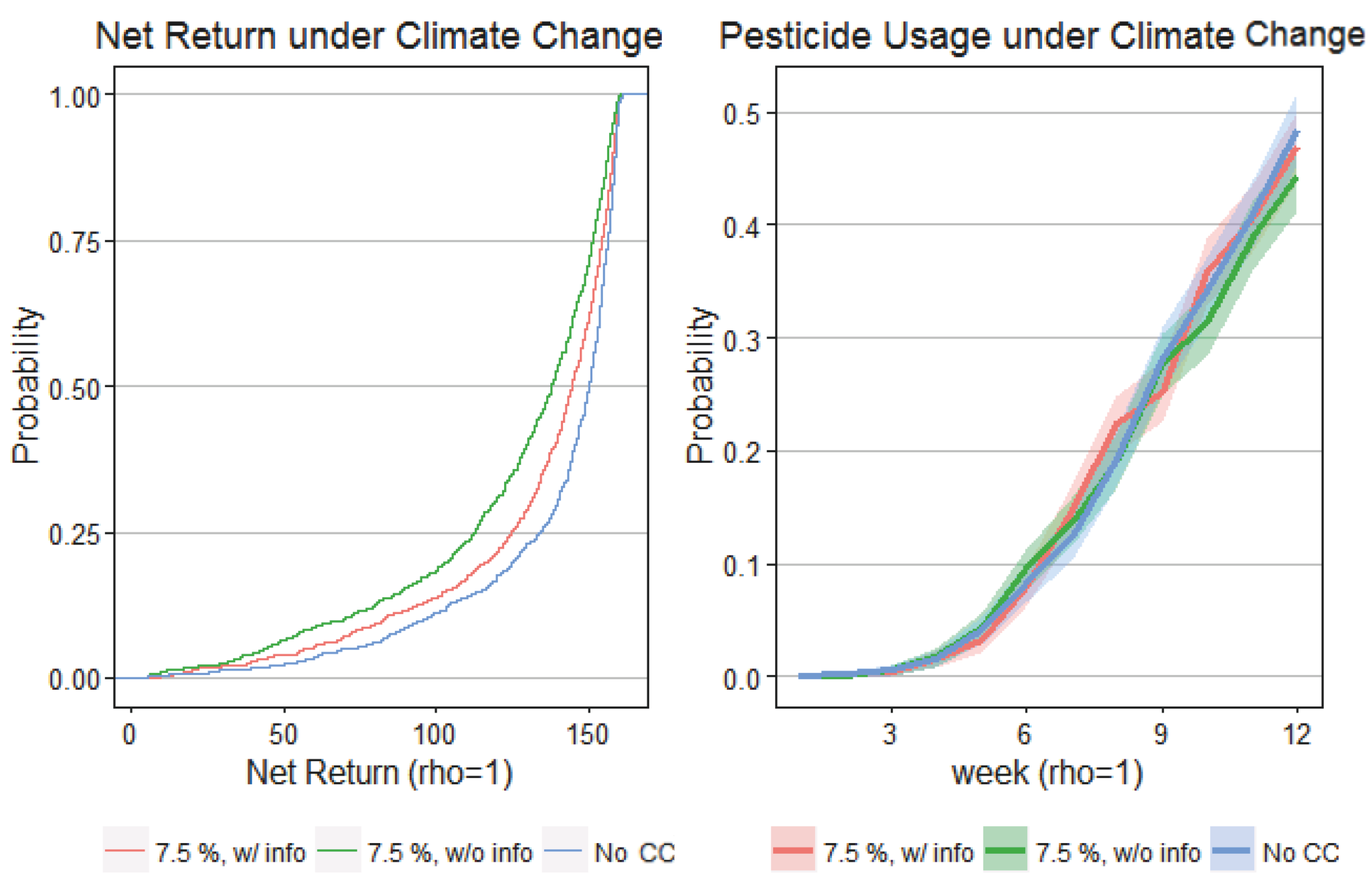
12	0.431	0.476	0.04 **	0.443	0.469	0.065 *
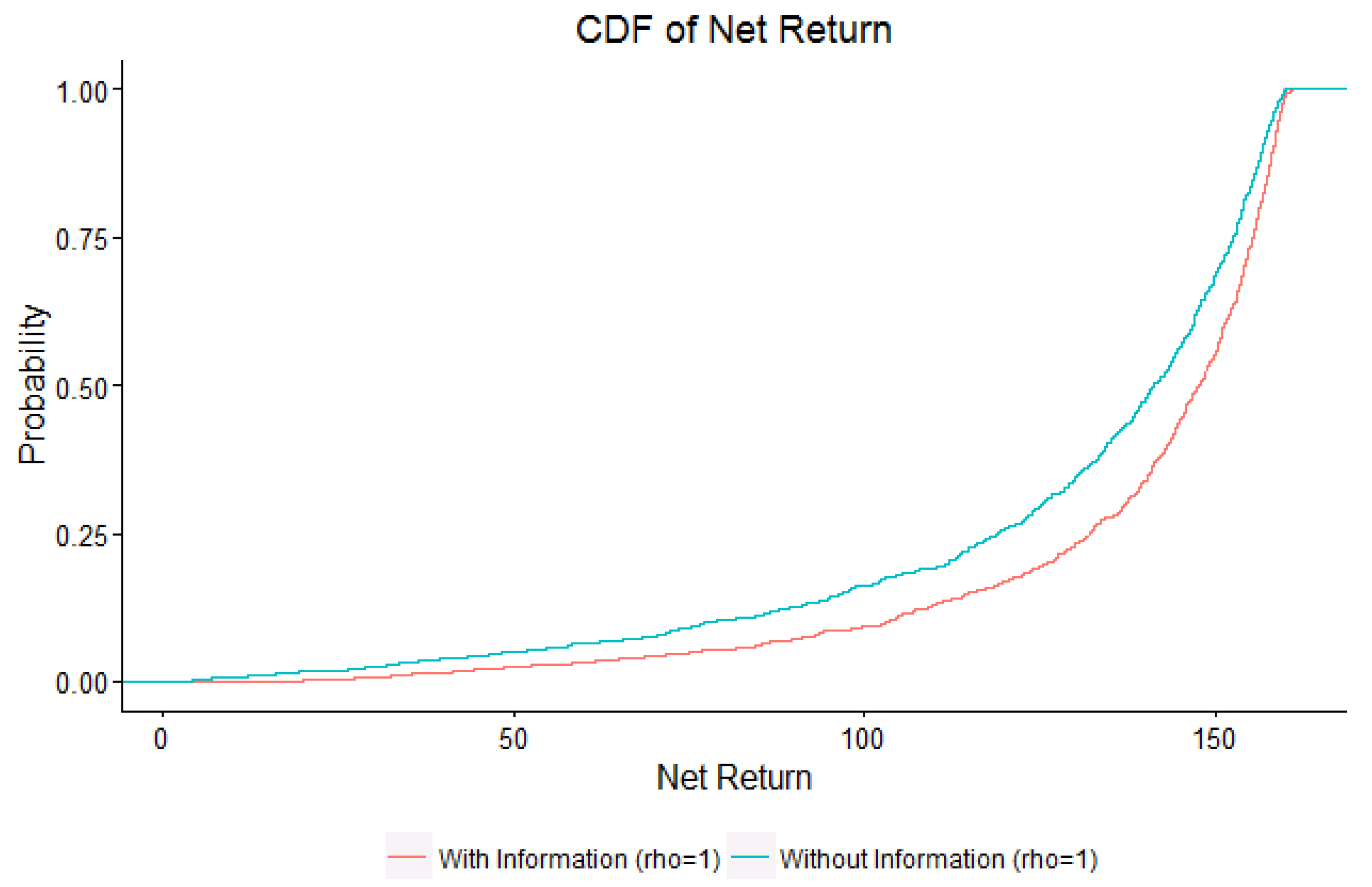
Expected	113.24	122.103	0.000 ***	94.25	106.49	0.008 ***
Net Return

Standard errors in parentheses. *** p < 0.01, ** p < 0.5, * p < 0.1.

provides the detailed simulated expected pesticide use and t-tests for the difference in pesticide application with and without $\rho$ information in each week. It should be noted that, when $\rho =0.5$, the main difference in usage comes from the last allowed spraying week. However, under alternative assumptions of value of $\rho$, the probability of spraying may also differ in week 6 and week 8 through 10. There is no significant difference in the probability of spraying in other weeks.

We examined the effect of non-zero correlation between volatility of weather and aphid outbreak on pesticide use for various values of correlation coefficients. We are also interested in the profit impact of taking the non-zero correlation into account in pest management activities. Difference in profits across solutions with and without considering non-zero correlation between weather and pest prediction errors in pest management decisions is equivalent to the value on information pertaining to the correlation coefficient. For a non-zero correlation coefficient between weather and pest population, we generate random draws of stochastic parameters and solve the model (a) assuming the correlation is zero, and (b) using the assumed value of the non-zero correlation. The results from the two corresponding solutions can be compared in terms of cumulative density functions of profits using the criterion of stochastic dominance. Figure A2 provides the cumulative distribution functions of a farmer’s per acre net benefit with and without the correlation coefficient information under different pest growth rate scenarios. It is clear that the net benefit of pest management with information about correlation coefficient between weather and pest population stochastically dominated the net benefits of pest management without consideration of the correlation between stochastic change in pest infestation and weather conditions.

On average, per acre, profits are $122.103 and $113.24 under pest management scenarios with and without information of the correlation coefficient (scenario of $\rho =0.5$). Therefore, the value of information(VOI) is $8.86 per acre, or approximately 7.8 percent of the profit. For the state of Idaho, where 30,000 acres of lentils were planted in 2012, this translates into $265,800 of total VOI.

2. Climate Change Scenario

The next scenario we consider is when there is climate change. In this article, we analyze a mild climate change scenario where the initial temperature of the growing season increases by $7.5$ percent, that is about 1.2 °C increment. Meanwhile, we also assume that the standard deviation of the weather stochastic process (${\sigma }^{\theta }$) increases by $7.5$ percent. Other parameters remain unchanged.

Figure A3 depicts the cumulative distribution of net return and pesticide use path under climate change. From the CDF plot, it is clear that the expected net return under climate change is below the scenario when climate change does not happen. In our model, this result is driven by the relative magnitude of the estimated yield growth rate (${\mu }^Y$) and pest infestation rate (${\mu }^A$). Compared to the no climate change scenario, the increment in pest infestation rate outpaces yield growth rate under climate change. Thus, it is unsurprising that net return declines. Meanwhile, due to faster pest infestation, farmers are forced to spray earlier in the growing season so that severe cumulative future damage on the biomass is prevented. In the case of $\rho =1$, the most significant difference between pesticide use path under climate change and no climate change happens in week 10, where the probability of spraying is much lower under climate change scenario. This significant drop is due to the fact that farmers are more likely to spray in week 7 and 8 under climate change.

A natural question to ask is: would VOI increase or decrease under climate change? A naive argument may suggest that the value of information decreases under climate change: from previous results, farmers without the correlation coefficient information tend to spray early and under climate change, farmers also should spray earlier. Thus, knowing the correlation coefficient shall be less important when climate becomes warmer. However, from Table A3 , it is clear that the VOI actually increased from $8.86$ dollars to $12.24$ dollars per acre. The reason lies in the probability of spraying in week 8 to 10. It is true that the difference in the probability of spraying between with and without the information declines in the final week. However, the difference is more spelled in week 8 to 10. When the farmer has the information, he or she assigns higher probability of spraying to week 8 and week 10 but one without such information assigns higher probability of spraying to week 9. Overall, our model suggests that, under climate change, not only do farmers have to spray earlier, but also their net returns are more sensitive to the choice of timing, which relies on gathering all relevant information.

5. Discussion and Conclusions

In this paper, we examine stochastic dynamic pest management in agricultural crop production with two stochastic factors that influence agricultural productivity: weather conditions and pest invasions. Predictions, or expected values, of weather conditions and pest invasions can be used in pest management practices. Furthermore, potential correlation coefficient between stochastic weather conditions and pest populations can be used to improve the effectiveness of pest management activities.

We first formulate a general dynamic discounted cost minimization problem with stochastic weather and pest population variables. We provide necessary conditions for optimal pesticide use trajectory during a growing season. Next, choosing functional forms that allow for mathematical tractability, we examine comparative dynamic properties of pest control activities as a function of the correlation coefficient between pest and weather forecast dynamics. Finally, we empirically examine pesticide use dynamics in the Palouse region of the Pacific Northwest, where reoccurring pea aphid invasions pose serious problems for the local lentil industry (See [15] for details).

This study extends the pest management literature by explicitly and simultaneously considering the dynamic influences of two stochastic factors: weather conditions and pest invasions. Furthermore, we account for potential correlation between stochastic weather and pest population dynamics in deriving optimal dynamic pest control trajectory in a growing season. These developments extend the works of [17,24] where only a single source of randomness was incorporated.

Our analytical results are confirmed empirically with respect to the potential importance of the correlation between stochastic weather and pest invasion dynamics in pest management. Our empirical results also demonstrate that applying pesticides later in the growing season could be preferred relative to earlier applications if pest spread rates are higher in later periods of growing season and if stochastically reoccurring invasions in later periods are possible. Pest growth rates in the later periods of the growing season can be higher than in the earlier periods because of more favorable habitat and weather conditions later in the growing season.

Future work from this study can go several directions. First, in this paper, we specify the correlation coefficient (${\rho }^{\tilde{A}\tilde{\theta }}$) as constant over time to simplify mathematical derivations. If the mathematical sophistication allows, one can examine how dynamic changes in the correlation between weather and pest outbreak could impact the results. Second, our scope of the analysis is limited to decisions within agricultural production stage. This work can be extended to analyze the exogenous effect from other agents along the agricultural supply chain (see for example [39,40,41,42] on lastest developments of modelling agricultural supply chains). Third, some of these relationships are estimated in this study using simple statistical methods. More sophisticated approaches for formulating these biophysical relationships, to be developed by professionals in the respective fields (especially the use of big data [43] and digital technologies [44]), will improve accuracy and reliability of predictions and corresponding correlation coefficient. Finally, an important element that should be incorporated into conceptual framework is growing pesticide resistance [45].

References

- Rose, S.K.; McCarl, B. Greenhouse gas emissions, stabilization and the inevitability of adaptation: Challenges for US agriculture. Choices 2008, 23, 15–18. [Google Scholar]
- Eigenbrode, S.; Capalbo, S.; Houston, L.; Johnson-Maynard, J.; Kruger, C.; Olen, B. Agriculture, Adaptation, and Mitigation. In Climate Change in the Northwest: Implications for Our Landscapes, Waters, and Communities; Chapter 6; Dalton, M., Mote, P.W., Snover, A.K., Eds.; Island Press: Washington, DC, USA, 2013; pp. 149–179. [Google Scholar]
- Kukal, M.S.; Irmak, S. Climate-driven crop yield and yield variability and climate change impacts on the US Great Plains agricultural production. Sci. Rep. 2018, 8, 3450. [Google Scholar] [CrossRef] [PubMed]
- Clement, S.L. Pea Aphid Outbreaks and Virus Epidemics on Peas in the U.S. Pacific Northwest: Histories, Mysteries, and Challenges. Plant Health Progress 2006, 7, 34. [Google Scholar] [CrossRef]
- Zilberman, D.; Schmitz, A.; Casterline, G.; Lichtenberg, E.; Siebert, J.B. The economics of pesticide use and regulation. Science 1991, 253, 518–522. [Google Scholar] [CrossRef]
- Carpentier, A.; Weaver, R.D. Damage Control Productivity: Why Econometrics Matters. Am. J. Agric. Econ. 1997, 79, 47–61. [Google Scholar] [CrossRef]
- Fox, G.; Weersink, A. Damage Control and Increasing Returns. Am. J. Agric. Econ. 1995, 77, 33–39. [Google Scholar] [CrossRef]
- Lichtenberg, E.; Zilberman, D. The Econometrics of Damage Control: Why Specification Matters. Am. J. Agric. Econ. 1986, 68, 261–273. [Google Scholar] [CrossRef]
- Saha, A.; Shumway, C.R.; Havenner, A. The Economics and Econometrics of Damage Control. Am. J. Agric. Econ. 1997, 79, 773–785. [Google Scholar] [CrossRef]
- Chen, C.C.; McCarl, B.A. Pesticide Usage as Influenced by Climate: A Statistical Investigation. Clim. Chang. 2001, 50, 475–487. [Google Scholar] [CrossRef]
- Chen, C.C.; McCarl, B.A.; Schimmelpfennig, D. Yield Variability as Influenced by Climate: A Statistical Investigation. Clim. Chang. 2004, 66, 239–261. [Google Scholar] [CrossRef]
- Costello, C.; Adams, R.; Polasky, S. The Value of El Niño Forecasts in the Management of Salmon: A Stochastic Dynamic Assessment. Am. J. Agric. Econ. 1998, 80, 765–777. [Google Scholar] [CrossRef]
- Rubas, D.J.; Mjelde, J.W.; Love, H.A.; Rosenthal, W. How Adoption Rates, Timing, and Ceilings Affect the Value of ENSO-based Climate Forecasts. Clim. Chang. 2008, 86, 235–256. [Google Scholar] [CrossRef]
- Cobourn, K.M.; Burrack, H.J.; Goodhue, R.E.; Williams, J.C.; Zalom, F.G. Implications of Simultaneity in A Physical Damage Function. J. Environ. Econ. Manag. 2011, 62, 278–289. [Google Scholar] [CrossRef]
- Elbakidze, L.; Lu, L.; Eigenbrode, S. Evaluating Vector-Virus-Yield Interactions for Peas and Lentils under Climatic Variability: A Limited Dependent Variable Analysis. J. Agric. Resour. Econ. 2011, 36, 504–520. [Google Scholar]
- Marsh, T.L.; Huffaker, R.G.; Long, G.E. Optimal Control of Vector-Virus-Plant Interactions: The Case of Potato Leafroll Virus Net Necrosis. Am. J. Agric. Econ. 2000, 82, 556–569. [Google Scholar] [CrossRef]
- Olson, L.; Roy, S. The Economics of Controlling A Stochastic Biological Invasion. Am. J. Agric. Econ. 2002, 84, 1311–1316. [Google Scholar] [CrossRef]
- Zhang, W.; Swinton, S.M. Incorporating Natural Enemies in An Economic Threshold for Dynamically Optimal Pest Management. Ecol. Model. 2009, 220, 1315–1324. [Google Scholar] [CrossRef]
- Zivin, J.; Hueth, B.M.; Zilberman, D. Managing a Multiple-Use Resource: The Case of Feral Pig Management in California Rangeland. J. Environ. Econ. Manag. 2000, 39, 189–204. [Google Scholar] [CrossRef]
- Hertzler, G. Dynamic Decisions under Risk: Application of Ito Stochastic Control in Agriculture. Am. J. Agric. Econ. 1991, 73, 1126–1137. [Google Scholar] [CrossRef]
- Richards, T.; Eaves, J.; Manfredo, M.; Naranjo, S.; Chu, C.; Henneberry, T. Spatial-Temporal Model of Insect Growth, Diffusion and Derivative Pricing. Am. J. Agric. Econ. 2005, 90, 962–978. [Google Scholar] [CrossRef]
- Saphores, J.D.M. The Economic Threshold with a Stochastic Pest Population: A Real Options Approach. Am. J. Agric. Econ. 2000, 82, 541–555. [Google Scholar] [CrossRef]
- Saphores, J.D.M.; Shogren, J.F. Managing Exotic Pests under Uncertainty: Optimal Control Actions and Bioeconomic Investigations. Ecol. Econ. 2005, 52, 327–339. [Google Scholar] [CrossRef]
- Sunding, D.; Zivin, J. Insect Population Dynamics, Pesticide Use, and Farmworker Health. Am. J. Agric. Econ. 2000, 82, 527–540. [Google Scholar] [CrossRef]
- Marten, A.L.; Moore, C.C. An options based bioeconomic model for biological and chemical control of invasive species. Ecol. Econ. 2011, 70, 2050–2061. [Google Scholar] [CrossRef]
- Sims, C.; Finnoff, D. When is a “wait and see” approach to invasive species justified? Resour. Energy Econ. 2013, 35, 235–255. [Google Scholar] [CrossRef]
- Clement, S.L.; Husebye, D.; Eigenbrode, S.D. Global Warming and Aphid Biodiversity: Patterns and Processes; Chapter Ecological factors influencing pea aphid outbreaks in the U.S. Pacific Northwest; Springer: Berlin/Heidelberg, Germany, 2010. [Google Scholar]
- Gan, Y.; Hanson, K.G.; Zentner, R.P.; Selles, F.; McDonald, C.L. Response of Lentil to Microbial Inoculation and Low Rates Offertilization in the Semiarid Canadian Prairies. Canaian J. Plant Sci. 2005, 85, 847–855. [Google Scholar] [CrossRef]
- Richards, T.J.; Manfredo, M.R.; Sanders, D.R. Pricing weather derivatives. Am. J. Agric. Econ. 2004, 86, 1005–1017. [Google Scholar] [CrossRef]
- Kamien, M.I.; Schwartz, N.L. Dynamic Optimization: The Calculus of Variations and Optimal Control in Economics and Management, 2nd ed.; Elsevier Science: Amsterdam, The Netherlands, 1991. [Google Scholar]
- Mbah, M.; Ndeffo, L.; Forster, G.A.; Wesseler, J.H.; Gilligan, C.A. Economically Optimal Timing for Crop Disease Control under Uncertainty: An Options Approach. J. R. Soc. Interface 2010, 7, 1421–1428. [Google Scholar] [CrossRef]
- Kao, E.P.C. An Introduction to Stochastic Processes; Duxbury Press: Belmont, CA, USA, 1996. [Google Scholar]
- USA Dry Pea And Lentil Council. U.S. Production Statistics; Technical Report; USA Dry Pea And Lentil Council: Moscow, ID, USA, 2007. [Google Scholar]
- Eigenbrode, S.; Bechinski, E.; Karasev, A.; Pappu, H.; Roberts, D.; Clayton, L.; McPhee, K.; Larsen, R.; Porter, L.; Stokes, B.; et al. Legume Virus Project. Technical Report. 2012. Available online: http://www.cals.uidaho.edu/aphidtracker/ (accessed on 7 June 2012).
- Siddiqui, W.H.; Barlow, C.A.; Randolph, P.A. Effects of some constant and alternating temperatures on population growth of the pea aphid, Acyrthosiphon pisum (Homoptera: Aphididae). Can. Entomol. 1973, 105, 145–156. [Google Scholar] [CrossRef]
- Ross, S.M. Introduction to Stochastic Dynamic Programming; Academic Press: Cambridge, MA, USA, 1995. [Google Scholar]
- EPA. Revised Interim Reregistration Eligibility Decisions for Dimethoate. Technical Report. 2011. Available online: http://www.epa.gov/oppsrrd1/REDs/dimethoate_ired_revised.pdf (accessed on 7 June 2012).
- EPA. Dimethoate 400. Technical Report. 2014. Available online: http://www.cdms.net/LDat/ld4PC014.pdf (accessed on 7 January 2014).
- Lu, L.; Winfree, J. Demand shocks and supply chain flexibility. In Proceedings of the NBER Conference “Risks in Agricultural Supply Chains”, Virtual Conference, 20–21 May 2021; Springer: Berlin/Heidelberg, Germany, 2021. [Google Scholar]
- Lu, L.; Nguyen, R.; Rahman, M.M.; Winfree, J. Demand Shocks and Supply Chain Resilience: An Agent-Based Modelling Approach and Application to the Potato Supply Chain; NBER: Cambridge, MA, USA, 2021. [Google Scholar]
- Rahman, M.M.; Nguyen, R.; Lu, L. Multi-level impacts of climate change and supply disruption events on a potato supply chain: An agent-based modeling approach. Agric. Syst. 2022, 201, 103469. [Google Scholar] [CrossRef]
- Zilberman, D.; Reardon, T.; Silver, J.; Lu, L.; Heiman, A. From the laboratory to the consumer: Innovation, supply chain, and adoption with applications to natural resources. Proc. Natl. Acad. Sci. USA 2022, 119, e2115880119. [Google Scholar] [CrossRef]
- Lu, L.; Tian, G.; Hatzenbuehler, P. How agricultural economists are using big data: A review. China Agric. Econ. Rev. 2022, ahead-of-print. [Google Scholar] [CrossRef]
- Du, X.; Wang, X.; Hatzenbuehler, P. Digital technology in agriculture: A review of issues, applications and methodologies. China Agric. Econ. Rev. 2022, ahead-of-print. [Google Scholar] [CrossRef]
- Ma, C.S.; Zhang, W.; Peng, Y.; Zhao, F.; Chang, X.Q.; Xing, K.; Zhu, L.; Ma, G.; Yang, H.P.; Rudolf, V.H. Climate warming promotes pesticide resistance through expanding overwintering range of a global pest. Nat. Commun. 2021, 12, 5351. [Google Scholar] [CrossRef]
- Yong, J.; Zhou, X.Y. Stochastic Controls-Hamiltonian Systems and HJB Equations; Springer: New York, NY, USA, 1999. [Google Scholar]
- Chang, F. Stochastic Optimization in Continuous Time; Cambridge University Press: Cambridge, UK, 2004. [Google Scholar]
- Oplinger, E.S.; Hardman, L.L.; Kaminski, A.R.; Kelling, K.A.; Doll, J.D. Lentil. Technical Report. 1990. Available online: http://www.hort.purdue.edu/newcrop/afcm/lentil.html (accessed on 30 June 2022).
- Painter, K. Crop Budgets. Technical Report. 2011. Available online: https://www.uidaho.edu/cals/idaho-agbiz/crop-budgets (accessed on 30 June 2022).
Publisher’s Note: MDPI stays neutral with regard to jurisdictional claims in published maps and institutional affiliations. |
© 2022 by the authors. Licensee MDPI, Basel, Switzerland. This article is an open access article distributed under the terms and conditions of the Creative Commons Attribution (CC BY) license (https://creativecommons.org/licenses/by/4.0/).
Share and Cite
Du, X.; Elbakidze, L.; Lu, L.; Taylor, R.G. Climate Smart Pest Management. Sustainability 2022, 14, 9832. https://doi.org/10.3390/su14169832
Du X, Elbakidze L, Lu L, Taylor RG. Climate Smart Pest Management. Sustainability. 2022; 14(16):9832. https://doi.org/10.3390/su14169832
Chicago/Turabian StyleDu, Xiaoxue, Levan Elbakidze, Liang Lu, and R. Garth Taylor. 2022. "Climate Smart Pest Management" Sustainability 14, no. 16: 9832. https://doi.org/10.3390/su14169832
APA StyleDu, X., Elbakidze, L., Lu, L., & Taylor, R. G. (2022). Climate Smart Pest Management. Sustainability, 14(16), 9832. https://doi.org/10.3390/su14169832