Lake Level Evolution of the Largest Freshwater Lake on the Mediterranean Islands through Drought Analysis and Machine Learning

Abstract

Vrana Lake on the karst island of Cres (Croatia) is the largest freshwater lake in the Mediterranean islands. The lake cryptodepression, filled with 220 million m³ of fresh drinking water, represents a specific karst phenomenon. To better understand the impact of water level change drivers, the occurrence of meteorological and hydrological droughts was analysed. Basic machine learning methods (ML) such as the multiple linear regression (MLR), multiple nonlinear regression (MNLR), and artificial neural network (ANN) were used to simulate water levels. Modelling was carried out considering annual inputs of precipitation, air temperature, and abstraction rate as well as their influential lags which were determined by auto-correlation and cross-correlation techniques. Hydrological droughts have been recorded since 1986, and after 2006 a series of mostly mild hot to moderate hot years was recorded. All three ML models have been trained to recognize extreme conditions in the form of less precipitation, high abstraction rate, and, consequently, low water levels in the testing (predicting) period. The best statistical indicators were achieved with the MNLR model. The methodologies applied in the study were found to be useful tools for the analysis of changes in water levels. Extended monitoring of water balance elements should precede any future increase in the abstraction rate.

1. Introduction

In recent decades, changes in water levels in rivers, lakes, aquifers, and in other reservoirs have been recorded worldwide. These changes are mainly associated with overexploitation of water caused by water consumption for agricultural irrigation, industry, tourism, or climate change, resulting in droughts and other water-related problems. All types of droughts originate from the deficiency of precipitation [1]. The extension of this deficiency over a long period of time is called a meteorological drought [2]. In contrast, hydrological, agricultural, and socioeconomic droughts highlight the interaction of the natural characteristics of a drought event and the human activities that depend on precipitation for adequate water supply to meet the societal and environmental demands [2]. In recent times, the research into hydrological droughts is increasingly linked to the study of trends that could be related to climate change [3,4,5].

The standardised precipitation index (SPI) developed by McKee et al. [6] is almost globally accepted as an indicator of the incidence and intensity of meteorological droughts. Hydrological droughts are defined using parameters similar to those used to define meteorological droughts [7], through various indices such as the Palmer drought severity index (PDSI) [8], surface water supply index (SWSI) [9], streamflow drought index (SDI) [7], standardised water level index (SWI) [10], and standardised groundwater level index (SGI) [11].

Water systems are complex, and simulations of runoff and water levels are challenging due to the large datasets required for model development and calibration. To date, analyses of water level changes have been performed using classical statistical methods. However, machine learning methods based on the interdependence of variables that allow the prediction of changes in water levels are being increasingly used. These methods offer the possibility to study the relationships between input variable (e.g., precipitation) and output variables, such as runoff or water level, without the need to build classical models and explicitly define physical relationships [12]. However, the implementation of machine learning models for the lake water level prediction is still at a development phase when compared with the physically based models [13]. Zhu et al. [13] point out that there are many questions about the application of the models, such as how to determine the input combinations to improve model reliability, how to split the available datasets to better capture water-level dynamics, or which model is more reliable. Most of the studies on lake water level forecasting have focused on daily or monthly water level dynamics, and have predicted water level fluctuations using only the past water level data as model input [13]. Akyuz and Cigizoglu [14] stated that the water level forecasts of various water bodies that are described in previous studies were analysed in the forecast range of 1 h to 30 months based on a time step of hourly to monthly values. As far as the authors are aware, only Noury et al. [15] have analysed annual variations of meteorological and hydrological variables (precipitation, temperature and river flow for several stations, and water levels in a period of delay of one year) as model inputs, and water level data of Urmia Lake (Iran) were considered as model outputs. To date, no accessible published studies exist that have considered the annual value of analysed variables and have used water pumping one of the inputs to the model.

There are many machine learning models that have been used to predict water levels. Artificial neural networks (ANNs) are one of the most commonly used methods in water resources research; see, e.g., [16,17,18,19,20,21,22,23,24]. They have been widely applied for lake water levels prediction [13,15,25,26,27,28,29,30]. Altunkaynak [25] used ANNs to analyse the level fluctuation of Van lake in Turkey and concluded that they are suitable because of their information processing characteristics, such as nonlinearity, parallelism, and noise tolerance, as well as their learning and generalization capabilities. Ondimu and Murase [26] applied ANNs to analyse Naivasha lake level in Kenya. Using the ANN and adaptive-neuro-fuzzy inference system (ANFIS) models, Yarar [27] analysed fluctuations of Beysehir lake level in southwestern Turkey. Water level variations of the Iznik lake in Turkey using ANNs, ANFIS, and gene expression programming (GEP) were analysed by Kisi et al. [28]. In recent times, as climate changes are becoming more pronounced, changes in water levels are linked to meteorological droughts. ML models have proven to be a useful tool in their prediction [31,32,33,34,35].

For Vrana lake level on the island of Cres, which is the subject of this study, a simulation of water levels based on monthly measurements of the water level in the lake over 38 years has been done using ANN, with results indicating an ability to predict water levels between 6–12 months in advance [36]. In contrast to the most commonly used daily and monthly input data for water level forecasting, we investigated the possibility of using annual available historical data of several variables that affect the lake level. The frequently applied ANN was also used, as well as less demanding methods such as the multiple linear regression (MLR) and multiple nonlinear regression (MNLR), which are less time-consuming and require minimal skill compared to the ANN technique [37,38,39].

The application of machine learning methods is often very complex due to the lack of input data, which is absent because monitoring has not been established, and due to the impossibility of measuring the indicators that are needed to create the model. This latter often refers to karst terrains, which on Earth occupy approximately 15.2% of the global land surface [40].

Vrana Lake on Cres Island, Croatia, is the largest freshwater karst lake in the Mediterranean islands and is only 3–4 km away from the sea. It is located in the northeastern part of the narrow Cres Island, which has an area of 405.7 km², making it the largest island in the Adriatic Sea. The lake is 5 km long with a maximum width of 1.45 km. The lake area is approximately 5.7 km², and it is at an average altitude of 12.78 m above sea level (a.s.l.) [41]. It contains 220 million m³ of fresh water. Because of its good water quality, the lake is used to supply water to the islands of Cres and Lošinj, and is the only source of drinking water for these islands with highly developed tourism. The water consumption rate is approximately 45–55 L/s during winter months, while over summer, it reaches approximately 150 L/s. The total abstraction rate from Lake Vrana in 2019 reached 2365.07 × 10³ m³, which is approximately 75 L/s. In many countries it is not always possible to satisfy increased water demands; pressure on karst aquifers will rise, and regulatory measures will be need to prevent or mitigate over-exploitation [42]. Fortunately, this still does not apply to the island of Cres, but it points the need for further research into this natural phenomenon with the application of new scientific methods, which is one of the main goals of this paper. The results of the work should contribute to the development of a better and more comprehensive monitoring system and the future sustainable management of this extremely valuable water supply resource in changed climatic conditions.

An extremely low water level of 9.11 m a.s.l. was recorded in 1990, which was a cause of great concern for experts and consumers of lake water regarding the future of the lake. Ožanić [43] determined that the recorded drop in water level was a consequence of an increased abstraction rate for water supply and the occurrence of unfavourable drought conditions over several consecutive years. Climate change has more recently been identified as a major problem affecting water resource sustainability, and the reduced water levels in Vrana Lake have primarily been attributed to rising air temperatures (and thus evaporation and evapotranspiration), then water abstraction, and only then annual precipitation [44]. These surveys were largely conducted using classic statistical methods.

A visual inspection of the available data showed a relatively stable water level from 1995, although the trend of increasing abstraction rates and air temperature is pronounced, and only a slight trend of increasing precipitation is indicated. The research goal was to investigate the possibility of evaluation and prediction of the lake water levels using available multi-year measured meteorological, hydrological, and anthropogenic data that represent water level drivers, and to apply the basic machine learning methods. The available data are related to precipitation, air temperature, abstraction rate, and lake water level. Evaporation from the surface of the lake and evapotranspiration from the land part of the basin were not considered due to the lack of continuous multi-year measurements. For this reason, additional attention was paid to the analysis of droughts. Another goal was to consider the possible reasons for the stabilization of the average lake’s water level after 1995.

There are several aspects in which our methodological approach differs from that of previous studies: (1) we used the standardised precipitation, water level, and air temperature indices (SPI, SWI, and STI, respectively) in the analysis of the changes in water levels; (2) we analysed the time series of the dependent and independent variables using the Mann–Kendall (MK) trend test, and auto- and cross-correlations; (3) we applied MLR, MNLR, and ANN methods to simulate the change in water level in the lake from the beginning of water abstraction; (4) we used annual data of precipitation, air temperature, and abstraction rate as well as the past lake level information as model inputs; and (5) we examined which input parameter contributed most to the water level change.

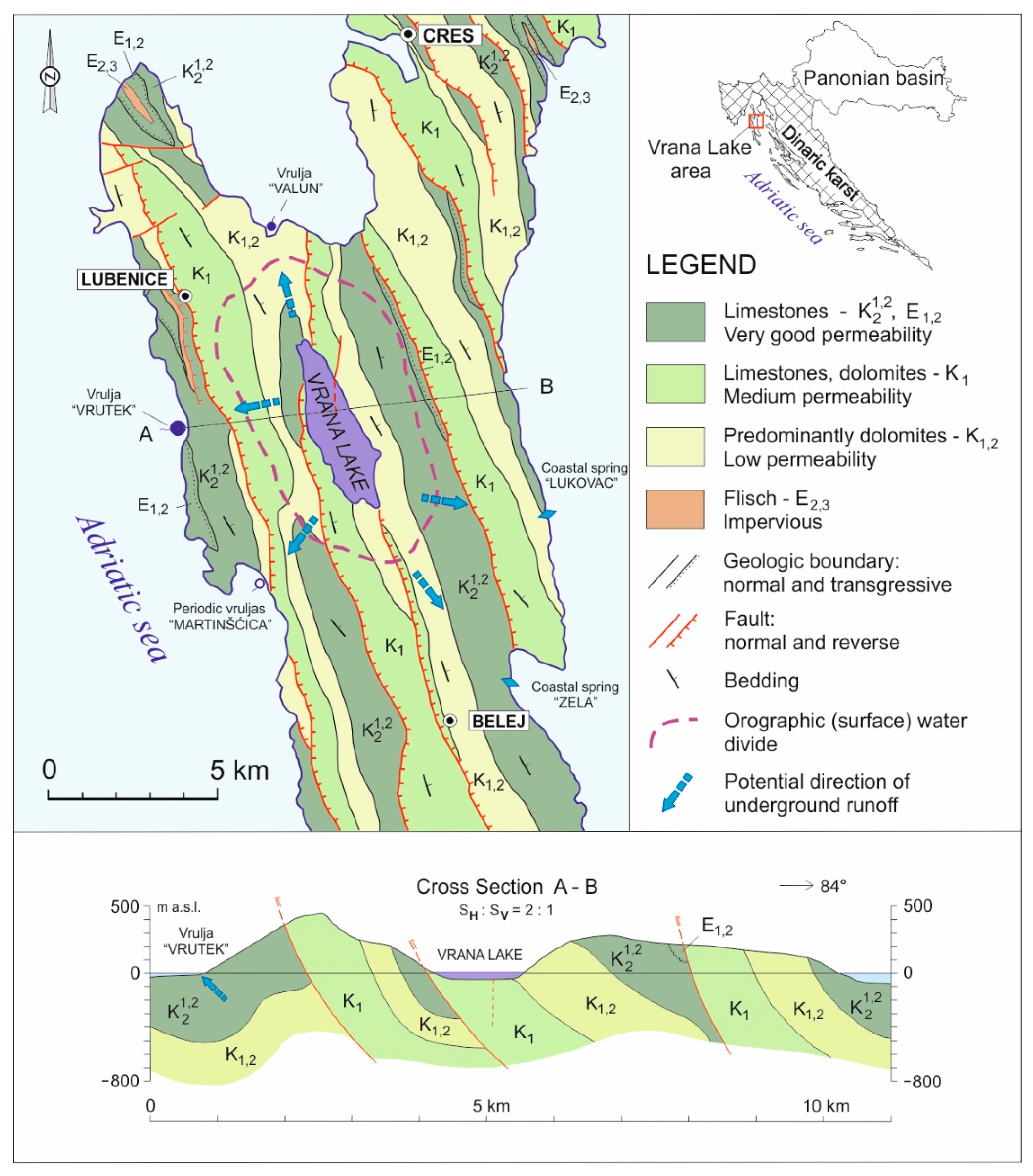
2. Geological and Hydrogeological Settings

Cres is a typical karst island mostly built of Cretaceous limestone and dolomite (Figure 1) which were deposited as part of a several thousand meter thick succession of carbonate sediments. The main geological structures formed during the orogeny of the Dinarides from the Late Cretaceous to the Miocene and were finally shaped by neotectonic movements. The genesis of Vrana Lake is related to the position of less permeable dolomite series (K_1,2), the influence of strike-slip tectonics (pull-apart structure), and the last sea level rise.

Vrana Lake is an oligotrophic lake, which was developed in a sensitive equilibrium with seawater, and represents a specific karst phenomenon. Vrana Lake is a submerged karst polje. The recent genetic phase followed the Würm glacial stage, when a global sea level rise of over 100 m resulted in a rise in groundwater levels in the remaining land areas. The lowering of the hydraulic gradient between the lake and the newly formed, elevated erosion base resulted in the slowing down of underground runoff and the significant closing of the previously developed drainage systems. This enabled the filling of the depression with fresh water and the forming of the recent Vrana Lake [46].

With the deepest point of 61.3 m below sea level, the lake is a cryptodepression without directly measurable surface or underground inflow and runoff. There is no permanent surface flow on the island, and even torrents active during heavy rains are rare, with only one occurring in the gully on the southern side of Lake Vrana. This torrent disappears shortly after the rain ceases.

The inhabitants of Cres Island and the surrounding islands previously consumed water from rare springs, dug wells, ponds, and cisterns, which is still the case on the smaller islands. Approximately 15 springs and 10 wells are present on the island of Cres, a majority of which are permanent, but have a low discharge rate that rarely surpasses 0.5 L/s. The wider coastal area of Cres Island has several submarine (called vruljas) and coastal springs (Figure 1). Some of these can be associated with Vrana Lake as possible privileged directions of lake discharge [47], which primarily refers to Vrutak vrulja, where, according to rough estimates, 50–250 L/s water flows out. However, tracing performed on the western side of the lake shore did not confirm this assumption [48]. On the eastern side of the lake, at a distance of up to 485 m from the lake, there are three observation wells in which groundwater levels are measured. Groundwater flows towards the lake and the hydraulic gradient ranges from 0.0048 in low water conditions to 0.1345 immediately after heavy rainfall [46].

3. Data and Methods

3.1. Data Source

The water level of Vrana Lake, precipitation, and air temperature have been officially measured since 1978 and 1981, respectively, by the Croatian Meteorological and Hydrological Institute (DHMZ). However, water levels between 1928 and 1978, as well as precipitation data before 1981, have been monitored by various researchers [43].

In this study, we used annual precipitation data for a period of 90 years from 1929 to 2019, and monthly precipitation data from 1981 to 2019. Annual and monthly air temperatures, which were measured for the period 1981–2019 at the Cres meteorological station, were also used. To model the water level of the lake, a series of mean annual air temperatures of Cres were extrapolated for the period 1954–1980 from data measured at the Rijeka meteorological station. This was possible because of the strong correlation coefficient (r = 0.975) between the mean annual air temperatures at both stations (Rijeka and Cres) during the period 1981–2013 [44]. In addition to the mean annual water levels from 1929 to 2019, the mean monthly water levels for the period 1978–2019 were analysed. Continuous monitoring of the abstraction rates has been done since the beginning of exploitation in 1954, and the data are recorded by the company Vodovod i odvodnja Cres-Lošinj d.o.o.

3.2. Calculation of the Standardised Drought Indices

The SPI was developed by McKee et al. [6] and provides a normalised measure as follows:

$$\mathrm{SPI}=\frac{P_i-P_{mean}}{S_P}$$

(1)

where P_i, P_mean, and S_P are the monthly precipitation, mean, and standard deviation, respectively.

The main advantage of SPI over other indices is that it allows not only the determination of the state of drought at different time scales but also the monitoring of different drought types [49]. According to SPI, droughts are classified into four classes: mild, moderate, severe, and extreme. A drought is described by SPI < 0, and excess precipitation over a period of time is described by SPI > 0. McKee et al. [6] determined that the SPI indicates mild, moderate, severe, and extreme drought 16–50%, 6.8–15.9%, 2.3–6.7%, and <72.3% of the time, respectively. The remaining values were allocated to the wet and normal classes. SPI is a standardised index; therefore, these percentages are expected from a normal SPI distribution.

McKee et al. [6] suggested that the equation used for calculating SPI could be applied to other variables relevant to drought, such as stream flow or groundwater. In this study, the SWI was used to represent hydrological drought and based on its value drought was categorised split into four classes that were the same as those for SPI [10]. Therefore, time series data on precipitation, air temperature, and water level were used to derive SPI, STI, and SWI, respectively. The STI and SWI build on the SPI of McKee et al. [6] to account for differences in the form and characteristics of air temperature and water level time series [50]. Extremely hot periods were marked with STI > 2 and extremely cold periods with STI < −2. High temperatures lead to increased evaporation from the water surface, contributing to the development of hydrological drought.

In this study, standardised indices were calculated using the cumulative precipitation and water level over different durations, for which the drought indices calculator (DrinC) software package [51] was used. Before the standardised index was assessed, monthly input data were used for gamma distribution calculation, and a log-normal distribution was used for the annual input data. In both cases, the obtained standardised indices followed a normal distribution. The percentages of droughts using the SPI and SWI indices were calculated for the period 1929–2019, as well as for three separate 30-year periods 1929–1958, 1959–1988, and 1989–2019.

From a hydrological point of view, the SPI, STI, and SWI were derived from the time series of monthly accumulated precipitation amount, mean monthly air temperature, and mean monthly water levels during the period 1981–2019, respectively. The recharge and discharge processes of the system are reflected in the SPI and SWI for 6-month periods within the hydrological year, from October to March, and April to September. The first period describes the recharge time and the second the discharge time of the system. SPI and SWI for these periods were also considered in this study.

3.3. Trend Analysis Method

The Mann–Kendall (MK) trend test [52,53] is a non-parametric test used to assess the significance of a trend and has been widely used in hydrological and meteorological trend detection studies [54]. The test was applied to the data as follows:

$$\mathrm{S}={\displaystyle \sum }_{i=0}^{n-1}{\displaystyle \sum }_{j=i+1}^{n}sgn\left(x_j-x_i\right)$$

(2)

where n is the length of the data set, x_i is from i = 1, 2, …, n − 1, and x_j is from j = i + 1, …, n. If n is greater than 8, then S approximates to normal distribution.

The annual precipitation and water levels, annual abstraction rate, and mean annual air temperature were analysed for several different periods. The MK trend test was used to statistically investigate whether there was a monotonic upward or downward trend in the variables (precipitation, air temperature, abstraction rate, and lake water level) over time. The significance levels at p < 0.05 are discussed. Kendall’s τ is a correlation coefficient and measure of the strength and direction of association that exists between two variables, where a positive τ-value indicates an upward trend and a negative τ-value indicates a downward trend. The data were analysed using XLSTAT software version 2021.4 [55].

3.4. Auto- and Cross-Correlation Method

Auto-correlation was used to analyse the effect of the previous year’s water levels on the current year’s water levels, and cross-correlation analyses were used to study the time lag between lake water level and precipitation, i.e., lake level and air temperature, and lake level and water abstraction rate. Analyses were performed using the XLSTAT software version 2021.4.

The auto-correlation coefficient r(k) was calculated for individual time lags k and is given by

$$r(k)=\frac{C_k}{C_0}$$

(3)

$$C_0=\frac{1}{n}{\displaystyle \sum _{i=1}^n(x_i-}\overline{x}{)}^2$$

(4)

$$C_k=\frac{1}{n}{\displaystyle \sum _{i=1}^{n\pm k}(x_i-}\overline{x})(x_{i+k}-\overline{x})$$

(5)

where x_i = (x₁, … x_n) is a time series of n data for which m auto-correlation coefficients, i.e., r(k) = (r₀, … r_m) are calculated.

The cross-correlation coefficient rxy(k) was calculated for the individual time lag k according to the following equations:

$$r_{x,y}(k)=\frac{C_{x,y}(k)}{{\sigma }_x{\sigma }_y}$$

(6)

$$C_{x,y}(k)=\frac{1}{n}{\displaystyle \sum _{i=1}^{n\pm k}(x_i-}\overline{x})(y_{i+k}-\overline{y)}$$

(7)

where σ_x and σ_y are the standard deviations of the input and output series, respectively.

3.5. Multiple Linear and Nonlinear Regressions

The influence of mean annual precipitation, air temperature, and abstraction rate on the water level in the lake was analysed using MLR and MNLR. The MLR describes the linear relationship between two or more independent variables and a dependent variable. The generic form of an MLR model is as follows [56]:

Y_MLR = c + β₁X₁ + β₂X₂ + … + β_nX_n

(8)

The MNLR model fits a nonlinear regression to the observed data [57], whose equations is as follows:

Y_MNLR = c + β₁X₁^β₂ + β₃X₂^β₄ + … + β_mX_n^β_m+1

(9)

In both equations, Y is the dependent variable, c is the intercept, X is the independent (explanatory) variable, β is the slope or unstandardized coefficient, and n is the number of input variables. In nonlinear models, m is the number of coefficients. The standardised coefficient β*, which is calculated by multiplying the unstandardized coefficient with the ratio of the standard deviations of the independent variable and dependent variable, was used in MLR to rank independent (explanatory) variables on the outcome of the dependent variable. A higher absolute value of the beta coefficient means a stronger effect of the variable. Coefficient standardization is important when independent variables or predictors are expressed in different dimensions.

In this study, analysis was carried out from the point when pumping began, for the period 1954–2019 using the software package XLSTAT version 2021.4 [55]. The mean annual water level (H) in the actual year was the dependent variable, and the mean annual precipitation (P), annual abstraction rate (Q), and mean annual air temperature (T) were independent variables. Precipitation and abstraction rates from previous years were added as independent variables based on cross-correlation analysis. The MLR and MNLR models were first applied for the analysis of data from 1954 to 2004 (training period), following which a water level prediction was made for the period 2005–2019 (testing period). Both models were also applied to the entire period 1954–2019 without splitting the data to the training and testing process. The aim of this modelling was to determine if there were any changes given that the distribution of water levels in the lake is very diverse over time.

3.6. Artificial Neural Networks

Changes in the lake water level were further analysed using ANN in the neuralnet package of XLSTAT version 2021.4 software (Paris, France) [55,58]. The lake water level prediction was driven by precipitation, air temperature, and abstraction rate, as well as their magnitudes in previous years (as previously described). The resilient backpropagation algorithm (Rprop), created by Riedmiller and Braun [59], was used to minimize the error function and to solve the problems of water level forecasting. The absolute partial derivatives of the error function with respect to the weight are used to find the minimum error. The iterative training process stops when all absolute partial derivatives of the error function are less than the given threshold which can be between 0.001 and 0.5. The network architecture consists of an input layer, a hidden layer, and an output layer. Different training datasets were tested to achieve the best possible modelling results while avoiding overfitting.

Two time series patterns were created in the input layer. The first is a recognition pattern consisting of the time series of average annual rainfall, air temperature, abstraction rate, and lake water level, which was used in the training process. Training covers the process of iterative input data were entered into the network, allowing the network to learn and adjust the trained data with the desired target data [60]. This includes determining the optimal interconnection weights and the number of hidden neurons. Initially, a time series from 1954 to 1999 was trained, but overfitting of the model was found. Avoiding overfitting was achieved by increasing the size of the training dataset, so the period 1954–2004 accepted for the training period, and the period 2004–2019 for the testing period. The same division into training and testing periods was used for the previously described two models, MLR and MNLR. A prediction pattern was used for the data testing process, which consisted of the time series of average annual rainfall, air temperature, and abstraction rate from 2005 to 2019. Thus, from the total data, 77% was used in the training process and 23% was used in the testing process. The ANN model was also applied to the period 1954–2019, without splitting the data to the training and testing process.

The mathematical model of information processing in a neuron is such that the inputs to the neurones (i = 1, …, n) receive input values x_i, which are real numbers. Each input value x_i is multiplied by the weight value w_ji, which describes the connection between input i and hidden neuron j, and then summed as per the following equation:

$$y_j={\displaystyle \sum }_{i=0}^n{w}_{ji}\times x_i$$

(10)

The obtained sum h_j is processed using the activation function of the hidden layer f (h_j) and the output from the neural network is equal to y_j.

$$y_j=f h_j$$

(11)

The prediction from the ANN model (y_k) can be expressed as follows:

$$y_j=f \left({\displaystyle \sum }_{j=0}^m{w}_{kj}\times h_j\right)$$

(12)

where w_kj is the connection weight between output neuron k and hidden neuron j, h_j is the output from neuron j in the hidden layer, m is the number of neurons in the hidden layer, and f is the activation function of the output layer.

In this study, one hidden layer was selected. The optimal number of neurons in the hidden layer, as well as the threshold was determined using a trial-and-error method until the best match between the observed and predicted water levels in the training and testing period was achieved.

The goodness of fit between the observed and simulated water levels in all the applied models was evaluated using the coefficient of determination (R²), mean absolute error (MAE), and root mean squared residual (RMSE), scatter index (SI), and bias:

$$R^2=1-\frac{{\displaystyle \sum }_{i=1}^n{\left(H_o-H_p\right)}^2}{{\displaystyle \sum }_{i=1}^n{\left(\overline{H_o}-H_o\right)}^2}$$

(13)

$$MAE=\frac{1}{n}{\displaystyle \sum }_{i=1}^n{\left|\left(H_o-H_p\right)\right|}_i$$

(14)

$$RMSE={\left[\frac{1}{n}{\displaystyle \sum }_{i=1}^n{\left(H_o-H_p\right)}_i^2\right]}^{0.5}$$

(15)

$$SI=\frac{RMSE}{\overline{H_o}}$$

(16)

$$Bias=\frac{1}{n}\sum \left(H_o-H_p\right)$$

(17)

where n is the number of observations, H_o is the observed water level, H_p is the predicted (simulated) water level, and $\overline{H_o}$ is the mean value of the observed water levels.

4. Results

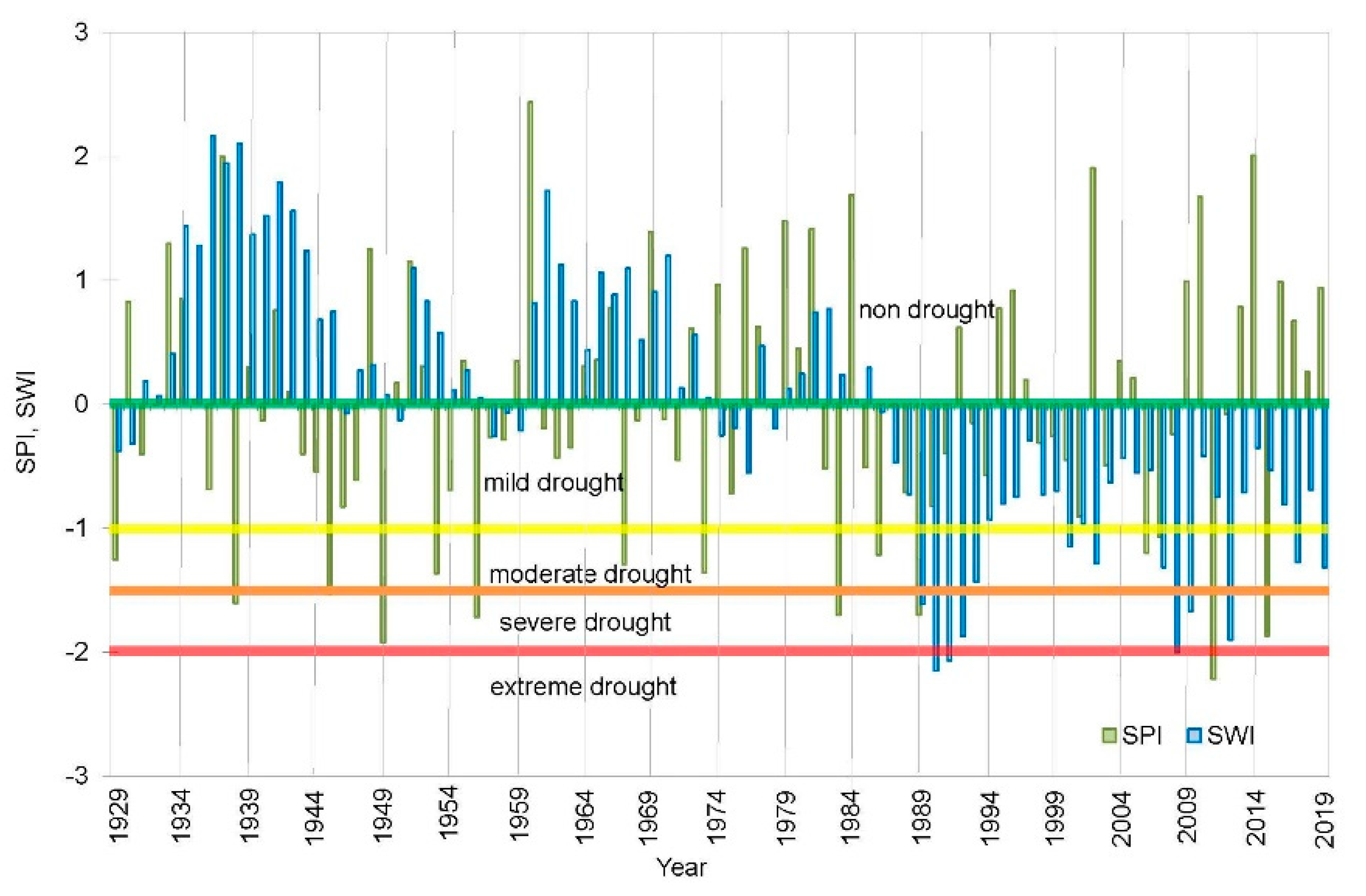
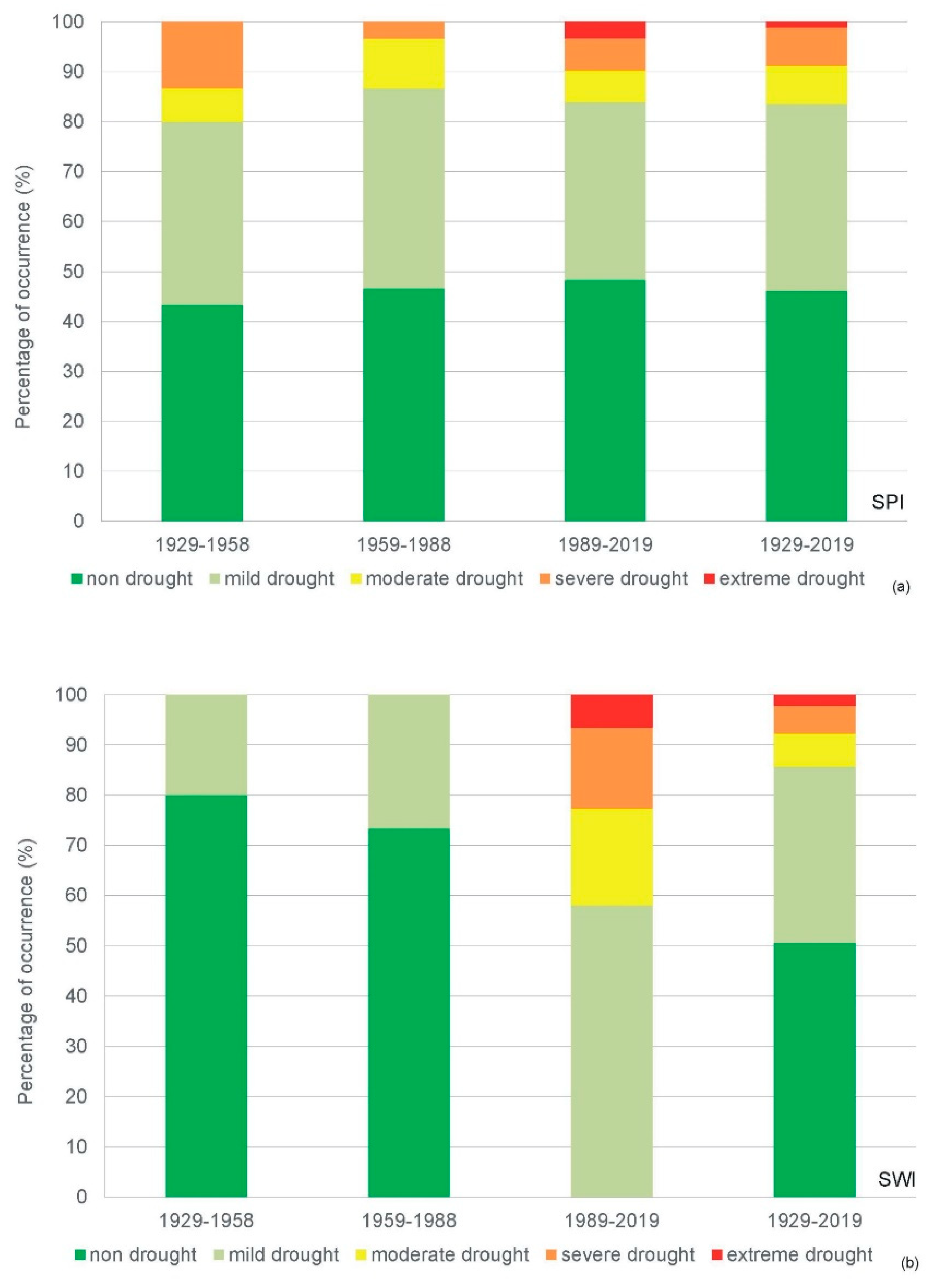
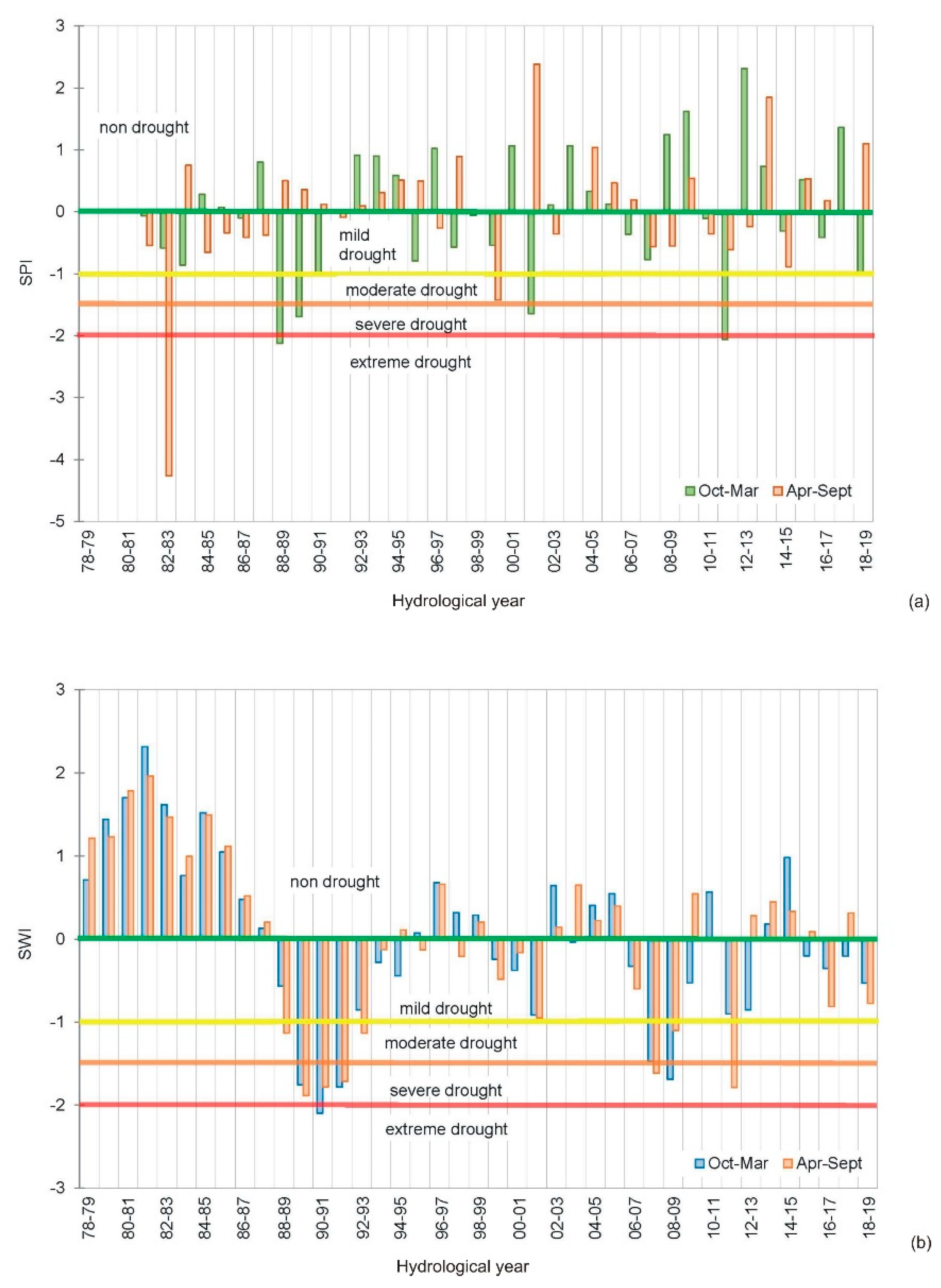
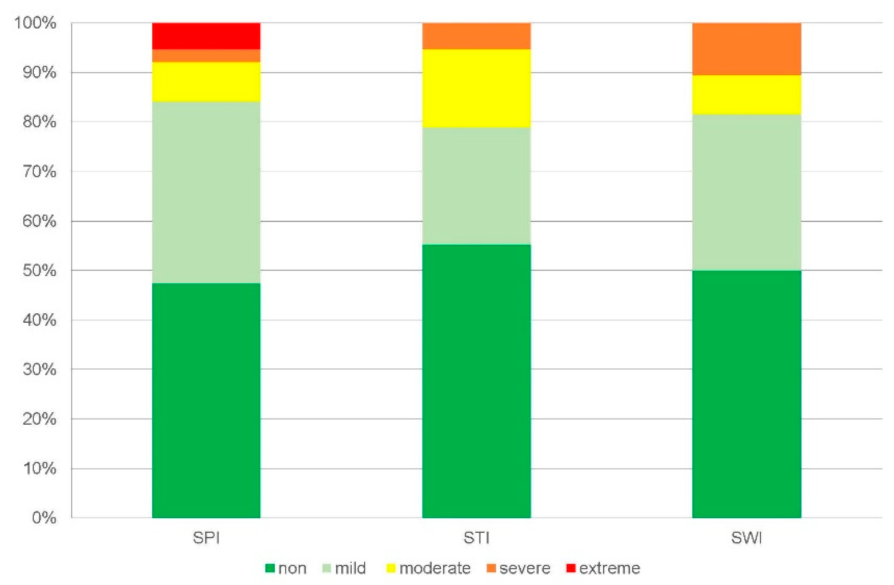
4.1. Changes in the Standardised Drought Indices

The SPI time series for the period 1929–2019 is presented in Figure 2. Though it appears that there was neither a significant increase nor decrease in the frequency of rainfall droughts, when comparing the three 30-year periods, a difference in the number and type of droughts was observed (Figure 3a). Four drought categories were registered from 1929 to 1958, the most common being mild drought (37%), followed by moderate drought (7%) and severe drought (13%). Furthermore, from 1959 to 1988, severe, moderate, and mild drought were recorded to have occurred 3%, 10%, and 40% of the time, respectively. During each time period, i.e., from 1929 to 1958 and from 1959 to 1988, drought was not registered 43% and 47% of the time, respectively. Similarly, the percentage of no-drought condition recorded in the period 1989–2019 was 48%. However, during the period from 1989 to 2019, extreme, severe, moderate, and mild drought were recorded at levels of 3%, 7%, 7%, and 35%, respectively. The resulting occurrence percentage of individual drought categories in the period 1929–2019 was approximately within the range reported by McKee et al. [6].

Unlike SPI, the SWI time series shows a marked change since 1986 (Figure 2). In the first two studied periods, 1929–1958 and 1959–1988, no hydrological drought was registered two-thirds of the time and a mild drought was registered one-thirds of the time (Figure 3b). However, after 1988, no-drought condition was not registered, and mild, moderate, severe, and extreme drought were registered 58%, 19%, 16%, and 7%, of the time, respectively (Figure 3b). The meteorological droughts recorded in the same period (Figure 3a) likely contributed to the higher prevalence of severe and extreme droughts; however, this is probably a consequence of the gradual increase in the abstraction rates.

Figure 4a,b show the SPI, SWI, and STI calculated on the basis of available average monthly values of precipitation, water level, and air temperature for the hydrological years 1981–2019 (38 years). According to the SPI, droughts that began in the early 1980s lasted almost a decade (Figure 4a), and until 1992 were mainly categorised as mild drought, although extreme drought was recorded in the hydrological year 82–83. Furthermore, a continuous dry period was observed from 1988 to 1991, falling mostly in the moderate drought category. Although the SPI has largely corresponded to non-drought since 1992, extremely dry years have occasionally been recorded in the hydrological years 99–00, 07–08, 11–12, and 14–15.

Unlike SPI, SWI was in the non-drought category at the beginning of the analysed period 1981–1988 (Figure 4a). However, from 1988 to 1993, drought was very pronounced in the hydrological years 89–90, 90–91, and 91–92. Since 1995, SWI has largely belonged to the non-drought class with an occasional but very pronounced decline in the severe to moderate drought class during the hydrological years 07–08, 08–09, and 11–12.

In the first 25 years of the observed period, from 1981 to 2006, the STI generally corresponded to the normal temperature class, and hot years were registered six times during that period, of which the moderate hot class was recorded twice (Figure 4b). Since 2007, the STI has generally shown a drought, which has belonged to the moderate hot class since 2013. A sharp global increase in air temperature was recorded in the 1980s, which corresponds with data presented in NOAA’s 2020 Annual Climate Report (https://www.ncdc.noaa.gov/sotc/global/202013 (accessed on 18 January 2022)), which suggest that the Earth’s temperature has risen since 1981. The years 2014–2020 were among the seven warmest years in Europe, which corresponds with the period when high air temperatures were recorded on Cres Island (Figure 4b).

No drought occurred as per any of the three indices approximately 50% of the time (Figure 5). Furthermore, the highest percentage of drought time refers to mild drought, and only the SPI was recorded in the extreme drought class. All three indices belonged to the drought-free and mild drought classes approximately 80% of the time; results for the remaining drought classes for the three indices were as follows: for the SPI, extreme, severe, and moderate drought classes were determined 5%, 3%, and 8%, of the time respectively; for the SWI, severe and moderate drought classes were determined 11% and 8%, of the time, respectively; and for the STI, moderate and severe hot classes were determined 16% and 5% of the time, respectively (Figure 5). The higher prevalence of severe drought as per the SWI is likely due to the lack of precipitation, i.e., the higher prevalence of severe SPI droughts.

Seasonal variations were analysed by dividing the hydrological years into winter (October–March) and summer (April–September) periods. According to the SPI, meteorological droughts were expressed through a decrease in summer precipitation in the first half of the 1980s and through a pronounced decrease in winter precipitation since 1987 (Figure 6a). Unlike the SPI, which, within the course of one hydrological year, may see an opposite sign in the winter from that in the summer, the SWI sign is generally identical (Figure 6b). From 1981 to 1988, the SWI for both 6-month periods belonged to the non-drought class, and from 1989 to 1994, the SWI for both 6-month periods belonged to the drought category, which reached the extreme drought class in the hydrological year 90–91. Pronounced meteorological droughts were recorded during the winter months in the hydrological years 88–89, 89–90, and 90–91 (Figure 6a), which otherwise represent the most significant time for lake water recharge. A pronounced lack of rainfall affected SWI droughts, which lasted twice as long as SPI droughts (Figure 6b). Droughts were also later registered in hydrological years 01–02, 07–08, 08–09, and 11–12, and were associated with concurrent meteorological (SPI) droughts.

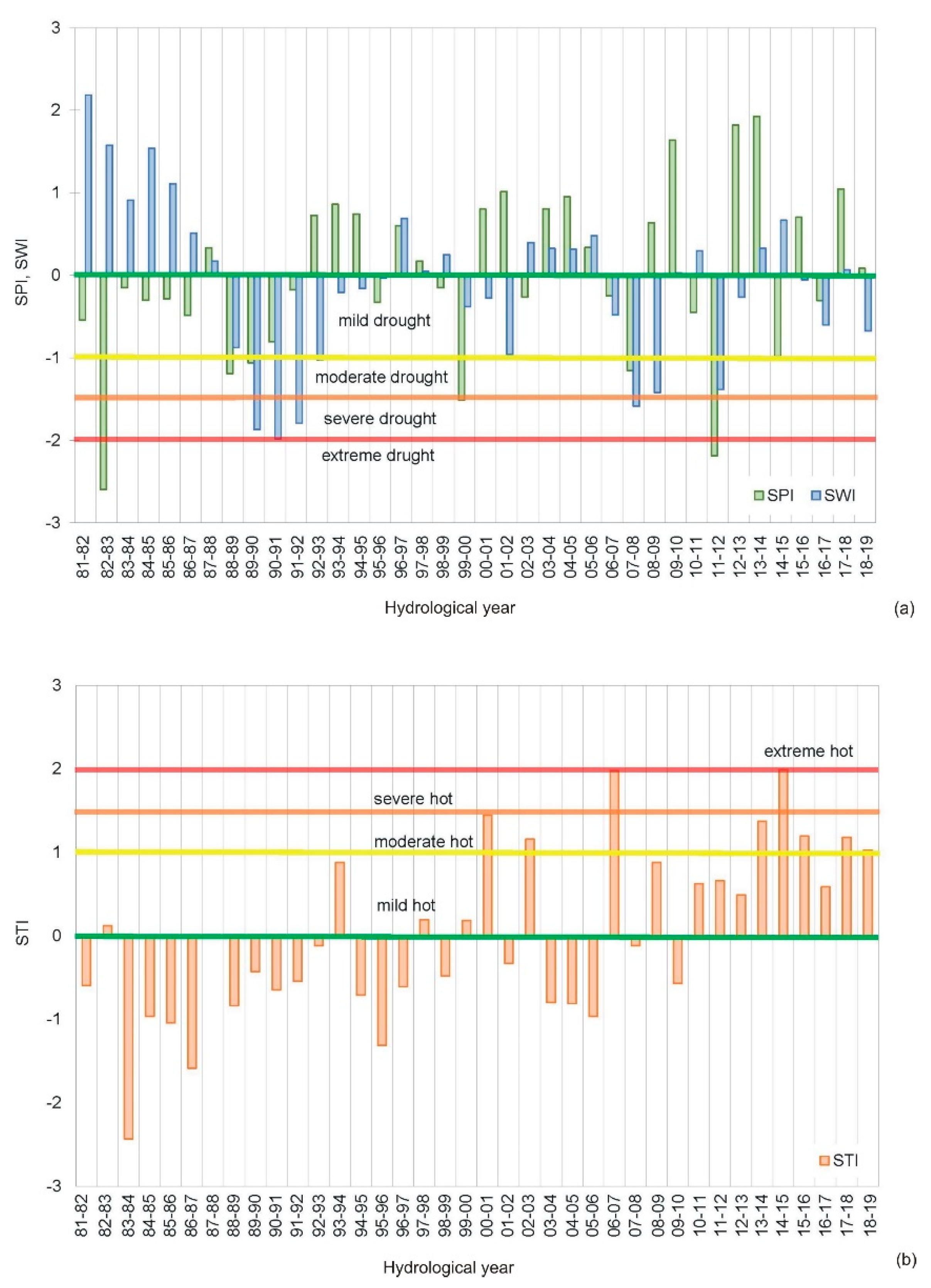
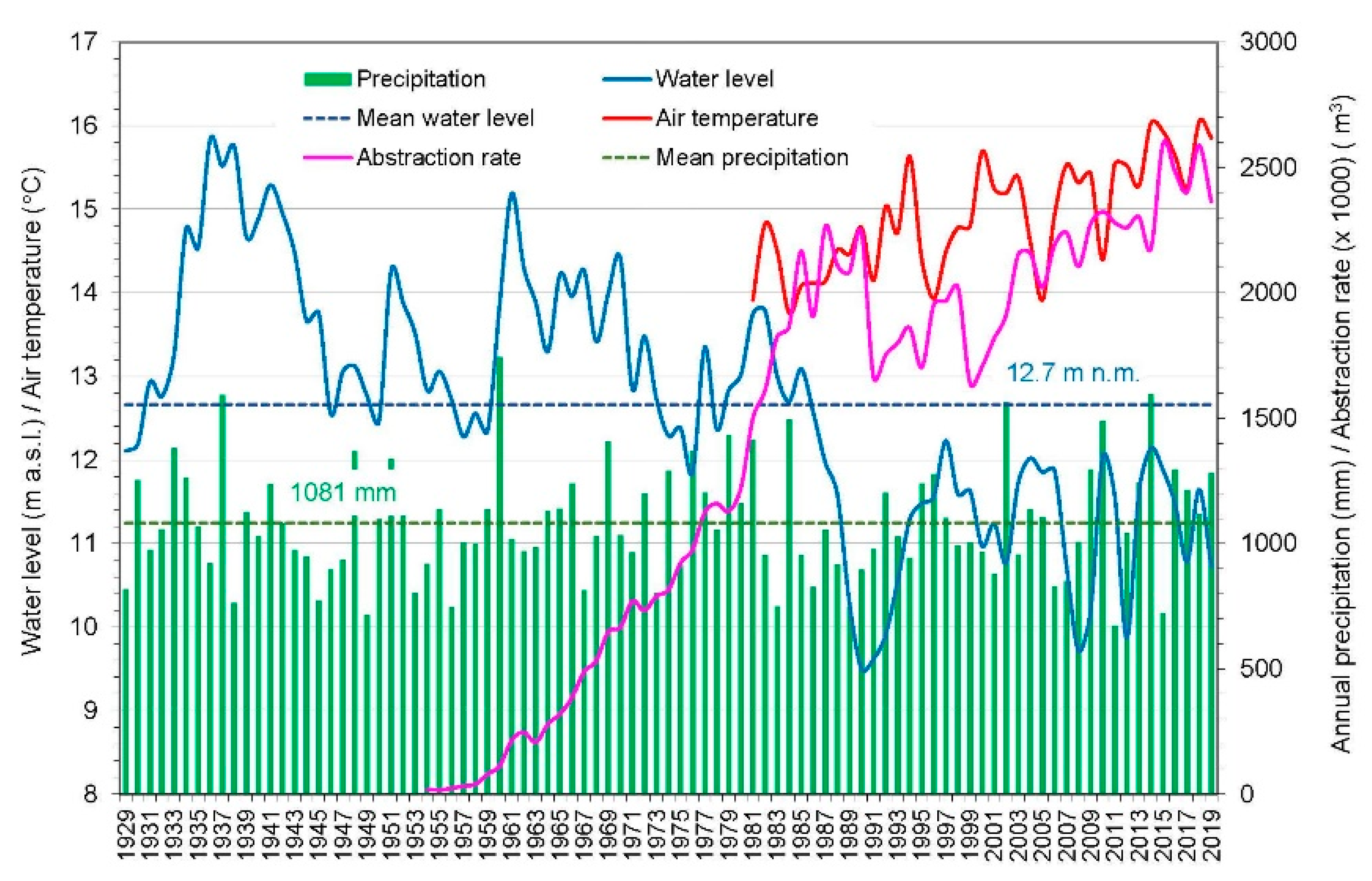
4.2. Time Series of Investigated Variables

The time series of annual precipitation (P), air temperature (T), abstraction rate (Q), and lake water level (H) are shown in Figure 7. The average water level of the lake during the study period was 12.7 m a.s.l. (Figure 7). Initially, it varied from 13 to 16 m a.s.l., after which a gradual decrease in water levels was recorded, culminating in 1990, when it was measured as only 9.11 m a.s.l. Thereafter, the water level in the lake was generally maintained between 11 and 12 m a.s.l. with two stronger drawdowns in 2008 and 2012. The average annual precipitation is 1081 mm, and air temperatures have gradually risen from 14 °C in the early 1980s to 16 °C in 2019 (Figure 7). The amount of abstracted water rose from approximately 1 L/s in 1954 to 71 L/s in 1990 when the Homeland War began. Since the end of the war in 1995, the amount of abstracted water has gradually increased to approximately 80 L/s.

Trends in these time series for different periods were examined using the MK trend test, and the results are presented in

Table 1. Mann–Kendall test results for time series of the mean annual precipitation (P), mean annual air temperature (T), mean annual abstraction rate (Q), and mean annual lake water level (H) in the different periods.

	Precipitation (P)	Air Temperature (T)	Water Level (H)	Abstraction Rate (Q)
Observation period	1929–2019
No. of data	91	39 *	91	66 **
p-value	0.472	<0.0001	<0.0001	<0.0001
Kendall’s τ	0.052	0.553	−0.529	0.844
Type of trend	n.s.s.	increasing	decreasing	increasing
Observation period	1929–1953
No. of data	25		25
p-value	0.455		0.726
Kendall’s τ	−0.110		−0.053
Type of trend	n.s.s.		n.s.s.
Observation period	1954–2019
No. of data	66	39 *	66	66
p-value	0.486	<0.0001	<0.0001	<0.0001
Kendall’s τ	0.059	0.553	−0.493	0.844
Type of trend	n.s.s.	increasing	decreasing	increasing
Observation period	1954–1990
No. of data	37	10 *	37	37
p-value	0.724	0.210	0.013	<0.0001
Kendall’s τ	−0.042	0.333	−0.287	0.964
Type of trend	n.s.s.	n.s.s.	decreasing	increasing
Observation period	1991–2019
No. of data	29	29	29	29
p-value	0.358	0.0005	0.293	<0.0001
Kendall’s τ	0.123	0.463	0.141	0.749
Type of trend	n.s.s.	increasing	n.s.s.	increasing
Observation period	1954–1981
No. of data	28		28	28
p-value	0.038		0.607	<0.0001
Kendall’s τ	0.280		−0.072	0.974
Type of trend	increasing		n.s.s.	increasing
Observation period	1982–1990
No. of data	9	9	9	9
p-value	0.466	0.466	0.001	0.029
Kendall’s τ	−0.222	0.222	−0.889	0.611
Type of trend	n.s.s.	n.s.s.	decreasing	increasing

* data since 1981. ** data since 1954. n.s.s.—not statistically significant.

. The following periods were analysed: (1) the entire period 1929–2019, (2) the period before the beginning of water abstraction from the lake (1929–1953), (3) the period from the beginning of the water abstraction (1954–2019), (4) the period from the beginning of water abstraction to the first large water level decrease (1954–1990), (5) the period after the first large water level decrease (1991–2019), (6) the period from the beginning of water abstraction to the first significant meteorological drought (1954–1981), and (7) the period from the first significant meteorological drought to the first large decrease in water level (1982–1990).

The results show positive (increasing) trends in air temperature and abstraction rate and a negative (decreasing) trend in water levels (p < 0.05). The trend of increasing mean annual air temperature has been monitored since 1991, and the trend of increasing mean annual abstraction rate has been monitored since the beginning of water abstraction in 1954. Increasing mean annual air temperature and abstraction rate (p < 0.05) can significantly contribute to decreasing mean annual lake water level. Furthermore, increasing the abstraction rate can lead to overexploitation and an increase in temperatures, which would lead to increased evaporation from the surface of the lake, and a lowering of water levels. No statistically significant trends were found for precipitation data during any of the analysed periods.

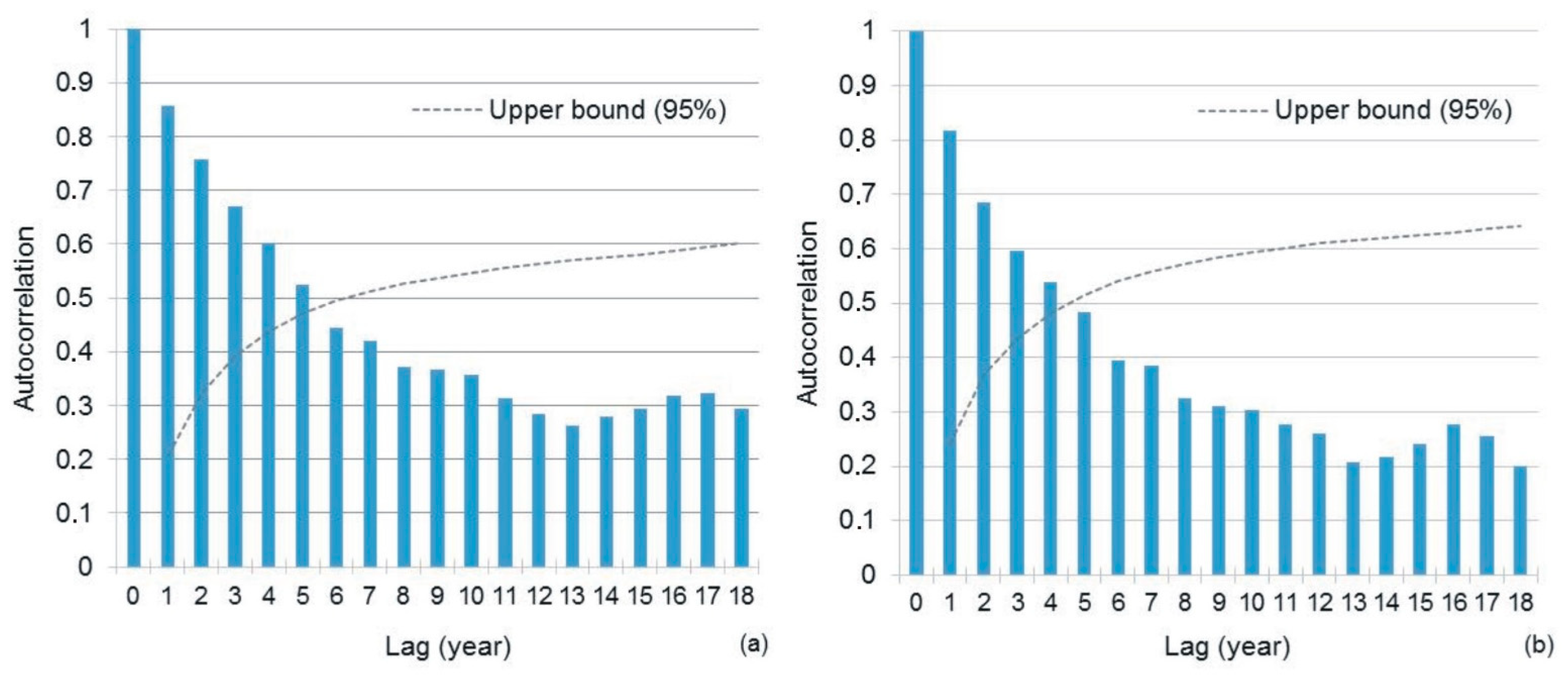
4.3. Auto-Correlation and Cross-Correlation of Variables

The auto-correlation coefficients for the water level in the periods 1929–2019 (n = 91) and 1954–2019 (n = 66) are shown in Figure 8. The annual water level fluctuation was time-dependent. For the period 1929–2019, the auto-correlation coefficients for a time interval of 1 to 5 years were higher than the upper bound of the 95% confidence interval. Furthermore, for the period 1954–2019, the time interval of auto-correlation coefficients above the upper bound of the 95% confidence interval was smaller, amounting to 4 years. Due to its dimensions, the lake was found to show marked sluggishness in the reactions [61]. Using auto-correlation analysis of average monthly water levels for the period 1929–1996, Ožanić et al. [61] found that a significant relationship between lake water levels lasted for 38 months.

The values of the cross-correlation coefficients between the lake water levels and precipitation, air temperature, and abstraction rate are summarised in

Table 2. Cross-correlation between lake water levels and three independent variables: precipitation (P), air temperature (T), and abstraction rate (Q).

Period	Correlation Coefficient (R)			Lag (Year)
	P	T	Q	P	T	Q
1929–2019	0.30	-	-	1	-	-
1954–2019	0.37	−0.35	−0.7 (±0.04)	1	0	<4

Not analysed due lack of data.

. Because the correlation coefficients are higher than in $\frac{2}{\sqrt{n-\left|k\right|}}$ where n is the number of observations and k is the lag, the correlation is significant. The best match between the time series of the annual abstraction rate and that of the annual water level in the lake was achieved with lags of up to 4 years. For these lags, the correlation coefficient was between 0.66 and 0.74, i.e., 0.7 (±0.04) as the average value. The time series of variables Q, Q_(t−1), Q(_t−2), Q_(t−3), and Q_(t−4) are very similar because of the gradual increase in abstraction rates. For precipitation and water level, the best matching was achieved with a lag of 1 year. There was no lag between the time series for air temperature and water level.

4.4. Developed Machine Learning Models

The selection of influential (significant) input variables in the development of MLR, MNLR, and ANN models is one of the most important steps [37]. Not all potential input variables are equally informative because some variables may be correlated, noisy, or have no significant relationship with the output to be modelled [62]. As previously mentioned, cross-correlation analysis of the annual data was performed to study the influence of precipitation, air temperature, and abstraction rate on the water level in the lake. This analysis showed a time lag of water levels behind precipitation of 1 year, behind an abstraction rate of up to 4 years, and no lag in the air temperature. Considering these findings, in addition to the variables P(t), T(t), and Q(t) for the considered year (t), the P_(t−1) and Q_(t−2) were used as input data for the MLR, MNLR, and ANN methods. The effect of evaporation was partially annulled by the introduction of air temperature because a pronounced increase in T causes water loss by evaporation from the lake surface. Owing to the typically strong auto-correlation of the water level time series, the simulated water level has been significantly influenced by past water levels. Therefore, the water level from the previous year, H_(t−1), was added as an explanatory variable.

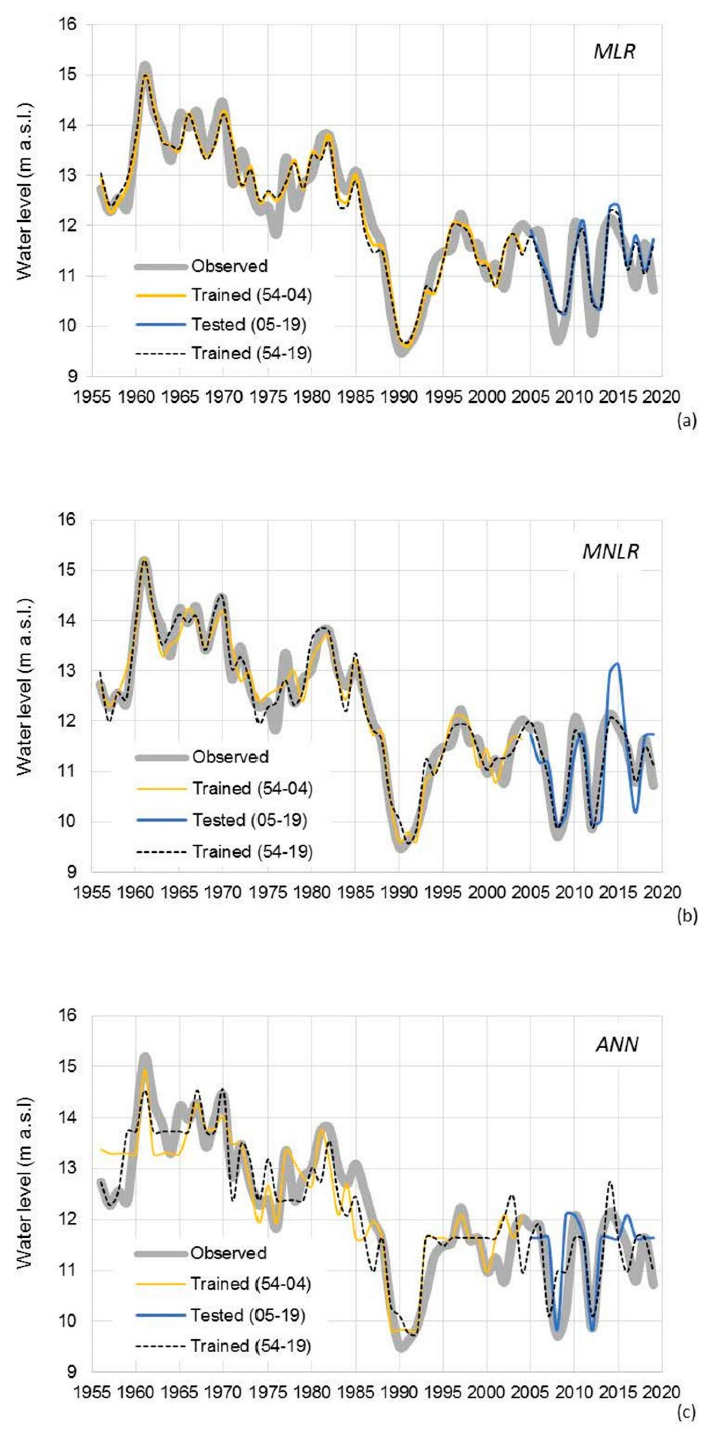
4.4.1. Multiple Linear Regression Model

Based on the six variables (P, T, Q, P_(t−1), Q_(t−2), and H_(t−1)), the best MLR model in the training phase (1954–2004) was achieved using the four independent variables P, P_(t−1), Q_(t−2), and H_(t−1). The R value between observed and simulated water levels was 0.95, MSE was 0.17 m, MAE was 0.34, and RMSE was 0.41 m (

Table 3. Goodness of fit between the observed and predicted water levels for the multiple linear regression (MLR), multiple nonlinear regression (MNLR), and artificial neural networks (ANN) models.

	Training Period (1954–2004)			Testing Period (2005–2019)			Training of Entire Period (1954–2019)
	MLR	MNLR	ANN	MLR	MNLR	ANN	MLR	MNLR	ANN
R2	0.90	0.93	0.82	0.42	0.50	0.43	0.89	0.96	0.81
R	0.95	0.96	0.90	0.65	0.71	0.66	0.94	0.98	0.90
MAE (m)	0.34	0.29	0.39	0.54	0.52	0.45	0.36	0.21	0.43
RMSE (m)	0.41	0.36	0.55	0.64	0.70	0.67	0.44	0.28	0.57
SI	0.033	0.029	0.045	0.057	0.062	0.060	0.036	0.023	0.047
Bias (m)	0.00	0.00	0.00	−0.13	−0.02	−0.28	0.00	0.00	0.00

). The equation for the MLR model obtained to simulate the water levels in the lake is as follows:

$$H=1.06+1.12\times {10}^{-3}\times P+3.58\times {10}^{-4}\times Q_{\left(t-2\right)}+1.94\times {10}^{-3}\times P_{\left(t-1\right)}+0.68\times H_{\left(t-1\right)}$$

(18)

The standardised coefficients (beta, β) of the independent variables in the MLR model show the relative contribution of each independent variable to the prediction of water levels (

Table 4. Standardised coefficients.

Variable	Beta	p-Value
P	0.187	0.0004
P(t−1)	0.323	<0.0001
Q(t−2)	−0.207	0.0004
H(t−1)	0.681	<0.0001

). The highest absolute value of the beta coefficient has variable H_(t−1), which means that the weight of this variable is more important. This is followed by variables P_(t−1) and Q_(t−2). These variables, as well as the P variable, were statistically significant (p < 0.05). The other two variables, T and Q, are not significant and therefore not included in this model. The R² value of 0.90 means that 90% of the variability of H is explained by the four variables P, P_(t−1), Q_(t−2), and H_(t−1).

The MLR model was tested for four assumptions that were required to be met in order for the model to be used for prediction [56]: (1) the linearity of the relationship between the dependent and independent variables, (2) independence of the errors (no auto-correlation), (3) homoscedasticity (constant variance) of the errors with respect to the predicted values, and (4) normality of the error distribution. The increasing spread of residuals with simulated values not been determined, so the assumption of constant variance of errors is satisfied (Supplementary Figure S1). The computed p-value of the Shapiro–Wilk test was 0.51, which is higher than the significance level of 0.05 and indicates that the residuals follow a normal distribution.

The auto-correlation of residuals was checked using the Durbin–Watson (DW) test [63]. In general, a DW statistic between 1.5 and 2.5 is used to conclude that there is no first-order temporal auto-correlation [64]. The value of the DW statistic for the obtained residuals was 2.7. Based on the read upper limit (dU) and lower limit (dL) at 5% of the significance level from the Savin and White table [65], it was determined that the DW value of 2.7 lies between the values of 4-dU and 4-dL (hence, (4-dU) < DW < (4-dL)), suggesting that the DW test was inconclusive.

The degree of multicollinearity was checked using the variance inflation factor (VIF) and tolerance. High multicollinearity corresponds to a VIF value >5 or a tolerance <0.2 [66]. The magnitudes of VIF and tolerance for all the independent variables used in developing the MLR model (Equation (18)) are between 1 and 2.4, and 0.4 and 0.9, respectively.

A water level prediction was made for the period 2005–2019. The R value between observed and predicted water level in the period 2005–2019 was 0.64, and the MAE, RMSE, and SI values were 0.54, 0.64 m, and 0.057, respectively.

In the conducted modelling the ratio of the testing data to the total length of data is 0.23. In a study by Zhu et al. [13], one quarter of the analysed publications had a ratio of testing data of approximately 0.23, and only 5% of them did not split the data for model evaluation.

In this study, the modelling was also conducted without splitting the data to the training and testing process. The aim of this modelling was to determine if there were any changes given that the distribution of water levels in the lake is very diverse over time. Six variables were retained in the model using the best variable selection method. The highest absolute value of the standardised beta coefficient has the variable Q_(t−2) (β = −0.753), suggesting that the weight of this variable is more important. This is followed by the variables H_(t−1) (β = 0.546) and P_(t−1) (β = 0.316). These variables, as well as the P variable, were statistically significant (p < 0.05). The beta coefficient of Q was 0.448, with a significance of p = 0.05. Furthermore, air temperature has slightly higher beta coefficient values (β = −0.063) in this period than in the period 1954–2004; however, it is still statistically insignificant (p = 0.244). It can be assumed that in the coming years, owing to climate change, the impact of air temperature will strengthen. Figure 4b clearly highlights the mostly mild to moderate increase in average air temperature since 2006 compared to the previous period. Investigating monthly climatic (precipitation, air temperature and evaporation), and management (abstraction rate) drivers of water level changes in Lake Bracciano near Rome, Italy, Guyennon et al. [30] also found a marginal role for temperature, an increasing role of abstraction during the past two decades, and a key role for increased precipitation variability. Negative values of the beta coefficients for the abstraction rate and air temperature indicate that an increase in pumping causes a decrease in the water level, and an increasing air temperature drives higher evaporation rates, also causing a decrease in the water level.

However, given that T and Q do not bring significant information to explain the variability of the dependent variable H, they were removed so the equation used to simulate the water levels in the lake is as follows:

$$H=2.1+1.19\times {10}^{-3}\times P-4.94\times {10}^{-4}\times Q_{\left(t-2\right)}+1.91\times {10}^{-3}\times P_{\left(t-1\right)}+0.6\times H_{\left(t-1\right)}$$

(19)

Indicators of the goodness of fit between the observed and simulated water levels for the period 1954–2019 are very similar to those for the period 1954–2004. The R value between observed and simulated water levels was 0.94, while the MAE, RMSE and SI were 0.36, 0.44 m, and 0.036 respectively (Table 3). All the assumptions that need to be met for the MLR model to be used for prediction are met, including the DW statistic which is on the top limit of validation and amounts to 2.52. However, the VIF values and tolerance for all the independent variables are between 1 and 2.2, and 0.4 and 1, respectively.

Using the MLR for the periods 1967–2013 and 1948–2015, Bonacci [44,67] found that the most important influence on the decreasing trend of the mean annual water level in Vrana Lake is the mean annual air temperature in relation to the abstraction rate and precipitation. According to the poorly described methodology of applying MLR in these articles, it follows that instead of a standardized coefficient, an unstandardized regression coefficient was used to define the influence of the analysed independent variables P (length, L), T (temperature, Θ) and Q (volume per time, L³T⁻¹) on the water level of the lake. However, the unstandardized coefficient should not be used to rank the independent variables to the outcome of the dependent variable because it does not eliminate dimensions.

4.4.2. Multiple Nonlinear Regression Model

The MNLR model was used to simulate the water levels in the lake in two steps. In both cases, a good match between the observed and simulated water levels was obtained using the polynomial equations. In the first step, the water level in the training period (1954–2004) was simulated and then forecasted for the testing period (2005–2019). Good results were achieved using third-order polynomials. The R value between the observed and simulated water levels for the training period was 0.96, and as in the MLR model, the R value was lower (0.71) for the testing period (Table 3). In the second step, a training process for the entire period under consideration (1954–2019) was performed, and the result was obtained using the polynomial equation of the seventh order. The R value between the observed and simulated water levels was 0.96, and the MAE, RMSE and SI were 0.21, 0.28 m and 0.023 which is significantly better than the value of these indicators for the MLR model (Table 3).

4.4.3. Artificial Neural Networks Model

The best ANN results were obtained using 36 hidden neurons. The training process (1954–2004) needed 20777 steps until all the absolute partial derivatives of the error function were smaller than 0.003. The R value decreased by approximately 0.24 between the training and testing (2005–2019) periods. The R value for the training and testing periods was 0.9 and 0.66, respectively (Table 3). In the second step, a training process was conducted for the entire period under consideration (1954–2019). Relatively good results were obtained using 32 neurons, and the threshold for the partial derivatives of the error function as stopping criteria was 0.003. The matching indicators of the observed and simulated water levels are very similar to the indicators for the entire period from 1954 to 2004 (Table 3).

5. Discussion

5.1. Comparison of Models

A relatively good matching of the observed and predicted water levels obtained using the MLR, MNLR, and ANN methods was observed (Figure 9). For the training period in all applied methods, the R value between the observed and simulated water levels was greater than 0.9, demonstrating a strong correlation (Table 3). A particularly strong correlation was determined using the MNLR model (R = 0.96), and the weakest correlation was that obtained using the ANN model (R = 0.91). In contrast to the preferred higher values of R² and R, a lower value of the regression model accuracy (MAE, RMSE and SI) implies a higher accuracy of the regression model. In both training periods (1954–2004 and 1954–2019), the MNLR model produced the lowest MAE (0.29 and 0.21), RMSE (0.36 and 0.28) and SI (0.029 and 0.023), and highest R² (0.93 and 0.96) and R (0.96 and 0.98) indicating that this method has a better fitting ability compared to the other two methods. Bias value for all models in the both training period is 0.00.

The R values for the applied models in the testing period were at the lower limit of the strong correlation, demonstrating a moderate predictive ability (Table 3). These values are very similar, varying around 0.7, and mirror the similar values of MAE, RMSE and SI. Bias values are varying between −0.02 for MNLR model to −0.28 to ANN model. However, in contrast to the training results, the MNLR model in the testing period showed significantly weaker prediction ability than expected (Table 3). The values of R² (0.5) and R (0.71) were significantly reduced, while the values of MAE (0.52), RMSE (0.7) and SI (0.062) were increased. Bias value for MNLR model in the testing period is very close to 0 (−0.02). For the MLR model, the bias is −0.13, and for the ANN model −0.28, which indicates a slight underestimation compared to observations. For instance, Figure 9b clearly shows that the simulated water levels in the MNLR model during the period 2013–2015 differ significantly from the observed water levels. The other two models also clearly show deviations of the simulated water levels from the observed values (Figure 9a,c). Based on the visual inspection of the observed and predicted water levels (Figure 9), as well as the indicators of the best match (Table 3), it is not possible to conclude with certainty which model gives the best results for the water level simulation in the testing period. Nevertheless, during the training period, all three models trained the impact of intensive water abstraction and less rainfall, which caused very low water levels in the early 1990s. As a result, in the testing period they recognised small amount of precipitation and high abstraction rate (Figure 2, Figure 4a and Figure 7), and correctly predicted a significant drop in water levels in 2008 and 2012 (Figure 9).

The modelling for the entire period 1954–2019 was performed using all three applied models, and the observed and predicted water levels match well (Figure 9). The training accuracy in the period 1954–2019 using the MNLR model has increased compared to the training accuracy in the period 1954–2004 to which the greater number of analyzed inputs probably contributed. However, this is not true for the MLR and ANN models. Their training accuracy in the period 1954–2019 is slightly reduced compared to the period 1954–2004 (Table 3). The R² values in the training period 1954–2004 of 0.9 for the MLR model, of 0.93 for the MNLR model and of 0.82 for the ANN model mean that 90% of the variability of H is explained by the four variables P, P_(t−1), Q_(t−2) and H_(t−1) in the MLR model, i.e., 93% in the MNLR model and 82% in the ANN model. For the training period 1954–2019, these four variables explain 89% of the variability in H in the MLR model, i.e., 96% in the MNLR model and 81% in the ANN model. Bonacci [37,61] found that the values of R of the MLR models in the periods 1967–2013 and 1948–2015 are 0.733 and 0.734, from which it follows that the value of R² is 0.54, i.e., that only 54% of the variability of the water level in the lake is explained by the analysed independent variables P, T and Q. The predictive ability in these articles was not tested, but considering that a relatively low percentage of the variability of H is explained by the analyzed variables P, T and Q, it can be assumed that during the testing period this model would show a very weak prediction ability the water level in the lake.

Figure 10 shows the distribution of the residuals obtained from the applied models for each model period: training (1954–2004), testing (2005–2019), and the entire period (1954–2019). Residuals were calculated each year by subtracting the simulated water level from the observed water level. A negative residual equals a rise in water level, and a positive residual represents a drop in water level. For all cases except the MLR model in the testing phase, the median residual value was almost zero (Figure 10). Four outliers were registered: two for the ANN model in the first training process (1954–2004) (box plot number 3 in Figure 10), one for the MNLR model in the testing process (2005–2019) (box plot number 5 in Figure 10), and one for the MNLR model in the second training process (1954–2019) (box plot number 8 in Figure 10). Both MNLR outliers referred to the same year. The residual values for the tested (2005–2019) and training processes (1954–2004) were 1.58 m and 0.74 m, respectively. Figure 9b clearly shows only the deviation registered in the testing process conducted in the period 2004–2019, but not in the training process conducted for the entire period of the research (1954–2019). Based on the Kolmogorov–Smirnov statistic, all residual distributions were found to be normal. Though considered a normal distribution, the ANN testing period (box plot number 6 in Figure 10) stands out, for which the p-value is only slightly higher than the significance level of 0.05.

Most of the published papers on the prediction of water levels in a lake by machine learning used daily or monthly data on water levels from previous years [13,36,68,69]. If in addition to water levels from previous years, meteorological data such as precipitation, air temperature, humidity, and wind were also used, and daily data were mainly analysed [39,70,71]. In such treatments, the time series contain a significant amount of data but describe relatively short periods (several years). Therefore, the prediction of water levels in the lake through the use of historical annual data of precipitation, air temperature, and abstraction rates, as well as water levels from the previous year, and using applied models is a novel contribution of this study. Annual data are particularly interesting from the perspective of analysing the impact of climate change on the availability of water resources. Unfortunately, the conducted analyses in this study have shown that the simulated water level of Vrana Lake is significantly influenced by the water levels in the past, which also was shown in the study of Noury et al. [15]. This suggests that the future impact of climate change or an increase in the abstraction rate on the lake water level cannot be reliably predicted by analysed annual input data (it is not possible to define level in the previous year for some future period because the water level is the target forecast variable).

The predictions obtained from this study were also compared with other published results. Noury et al. [15] used support vector machines (SVM) and neural wavelet network (NWN) models to predict the annual water level in Lake Urmia. The results of the SVM model were better (R² = 0.97) than those obtained with the NWN model (R² = 0.95). Annual input data being used for time series analysis is not only a rarity in the research of lake water level variations, but also in the research of time series of other hydrological variables. Shiri and Kisi [72] investigated the use of daily, monthly, and annual streamflow data using single neuro-fuzzy (NF) and wavelet-neuro-fuzzy (WNF) models. For the test period in both models, the best results were achieved using daily and monthly input data, but they are somewhat worse for the NF model compared to the WNF model. However, for annual input data, the results of the NF model were significantly worse than the results of the WNF model; Pearson’s correlation coefficient was −0.338 in the NF model, and 0.994 in the WNF model. The authors concluded that a model architecture that works well on one case does not necessarily work on another. The results obtained in our study, as well as the results of other described studies, point to the need for further research. Other modern forecasting methods should certainly be applied in order to find the best method for water level forecasting with applied input data.

5.2. Impact on the Water Level of Vrana Lake

Before the start of water abstraction from Vrana Lake (1929–1953), no trends in precipitation or water levels were observed (Table 1), and no significant stress that would have caused a drawdown of the water level in the lake was noted. A constant record of the abstraction rate has existed since 1954 (Figure 7). For the period 1954–2019, the results of the MK trend test show that there are positive (increasing) trends for air temperature and abstraction rate and a negative (decreasing) trend for water level at a significance level of p < 0.0001 (Table 1). The precipitation data for this period did not show a significant change trend. The Kendall’s τ coefficient for the abstraction rate, air temperature, and water level were 0.84, 0.55, and −0.49, respectively (Table 1).

Ožanić [44] and Ožanić and Rubinić [47] using a mathematical-hydrological model found that in the period 1929–1997 the average annual inflow was 18.5 × 10⁶ m³, the average evaporation from the lake surface 6.7 × 10⁶ m³, and the average annual underground runoff (losses) from the lake was approximately 11.7 × 10⁶ m³. The average annual water level in the lake was 13.10 m a.s.l. Owing to the large area of the lake in relation to the catchment area, 33% of the total inflow into the lake is from precipitation that falls directly on the surface of the lake, and the remainder is underground recharge from the catchment area. According to the results of the modelling, the authors determined that the surface of the catchment area that optimally satisfied the water balance conditions was approximately 24 km².

The first lowering of the lake’s water level to 9.5 m a.s.l. was registered in 1990 (Figure 7). To discern what led to this phenomenon, the pumping period was divided into several shorter periods. From the beginning of pumping to 1990, the MK test showed a significant trend of increasing abstraction rates (Kendall’s τ is 0.964, p < 0.0001), which followed a significant trend of lowering the water level of the lake (Kendall’s τ = −0.287, p = 0.013) (Table 1). Precipitation and air temperature did not show any significant trends, with temperature measurements beginning in 1981.

Since 1982, the water level of the lake has decreased, which is clearly visible in Figure 4a, Figure 6b and Figure 7. The results of the MK test for the period 1982–1990 showed that the trend of increasing abstraction rates (p = 0.029) affected the decrease in water levels (p = 0.001) (Table 1). The Kendall’s τ coefficient for the abstraction rate and water level are 0.61 and −0.89, respectively. In the period 1982–1990, the abstraction rate increased from 1.6 × 10⁶ m³/year to 2.2 × 10⁶ m³/year (by approximately 40%), and the water level decreased from 13.8 m a.s.l. at 9.5 m a.s.l. (by approximately 30%). Precipitation and air temperature did not show any significant trend. Precipitation in this entire period mainly reflected drought (Figure 4a) with no noticeable trend. The air temperature did not show drought, also without a clearly expressed trend (Figure 4b). Prior to 1982, no significant trends in the changes in the water level of the lake were found (Table 1), although the trend of increasing abstraction rates (p > 0.0001) was significant. Mean annual abstraction rates in that period increased from 0.14 × 10⁶ m³ in 1967 to 1.6 × 10⁶ m³ in 1982.

Despite the trend of increasing abstraction rates (p < 0.0001), as well as the increase in air temperature (p = 0.0005) which affects the increase in evaporation rate from the lake surface and evapotranspiration in the catchment area, the trend of lake water level in the period 1991–2019 was not statistically significant. The average annual water level of the lake in the period 1991–2019 was lower by 0.9 m than in the period 1982–1990 (

Table 5. Average annual values of analysed variables in different time periods.

Period	Hav (m a.s.l)	Pav (mm)	Tav (°C)	Qav (×106) (m3)
1954–1981	13.3	1115.9	13.9	0.55
1954–1990	13.0	1076.5	14.3	0.91
1982–1990	12.1	954.0	14.4	2.01
1991–2019	11.2	1104.3	15.1	2.09

). Though the water level increased after the low level observed in 1990, it did not reach the same level, and has been maintained at an average of 11.3 m a.s.l. since 1995 (Figure 7). The abstraction rate increased from 1.7 × 10⁶ m³ in 1991 to approximately 2.5 × 10⁶ m³ in 2018. However, the average annual abstraction rate in that period was very similar to that in the period 1982–1990, when there was a sharp drawdown in the water level of the lake (Table 5). In the same period (1991–2019), the average annual rainfall was almost 16% higher than that in the period 1982–1990. Based on these observations, it can be assumed that new water balance conditions have been established which, with an increase in precipitation, enable the same abstraction rate at a lower water level. Lower water levels and the associated reduction of the hydraulic gradient towards the sea have reduced underground runoff (losses) from the lake. A gradient of change underground runoff per each meter of water level was estimated at approximately 0.028 m³/s (0.88 × 10⁶ m³/year) [47]. The average water level in the period 1991–2019 was 0.9 m lower compared to the average water level in the period 1982–1990, which means that these losses are reduced by approximately 0.8 × 10⁶ m³. Furthermore, Bonacci [44] found that an increase in annual air temperature of 1 °C increases evaporation by approximately 0.5 × 10⁶ m³ of water. The average air temperature in the period 1991–2019 was 0.7 higher than the average air temperature in the period 1982–1990 (Table 5). Assuming linear relationships, this would mean that evaporation in the period 1991–2019 increased by 0.35 × 10⁶ m³. Based on these relationships, it can be assumed that the losses related to underground runoff from the lake and evaporation reduced by 0.45 × 10⁶ m³ in the period 1991–2019 in relation to the period 1982–1990. At the same time, it is possible that the underground recharge from the surrounding aquifer increased as a result of the increase in the catchment area, i.e., the increase in the cone of depression due to the lower level of the lake. During the period 1982–1990, the average rainfall was 13.5% less, and the average abstraction rate was approximately 4% less than that in the period 1991–2019. Still, such an abstraction rate, with the occurrence of unfavourable hydrological conditions (Figure 4a and Figure 6b), caused the appearance of very low water levels, as recorded in 2008 and 2012 (Figure 7 and Figure 9).

5.3. Limitations

It should also be considered that the water level in the lake is not only influenced by the herein used variables, but also by other elements of water balance, such as evaporation, evapotranspiration, and underground runoff from the lake. Since these data were not used in this study, it is expected that their inclusion in future machine learning models could contribute to a better prediction of lake water level and lead to lower statistical error, as shown by Buyukyildiz et al. [73]. If all the input elements affecting the water level of the lake were known, the output data from the model would be the height difference between successive annual lake water levels, as shown in the mentioned paper.

5.4. Practical Implications

The first hydrological analyses of Vrana Lake, carried out at the time of the start of pumping for public water supply, predicted the possibility of a mean annual abstraction rate of 250 L/s [74]. Analyses carried out after the occurrence of a large drop in the lake level in 1989 showed that these quantities were overestimated and suggested that the sustainable pumping capacity likely should not exceed 90 L/s [43].

The results of the analyses presented in this paper point to significant changes in environmental conditions that are probably the result of global climate changes. In the last thirty years, the frequent occurrence of dry years (SWI on Figure 2), and a significant increase in average annual air temperatures, especially after 2006 (STI on Figure 4b, and Figure 7), is indicative. Likewise, the applied machine learning models showed a significant influence of the abstraction on the lake level. The obtained results show that any further increase in the abstraction rates should be carried out with caution. It is very likely that in the changed hydrological conditions, the sustainable abstraction rates are less than 90 L/s, and today’s mean annual abstraction rate of approximately 82 L/s is very close to the maximum sustainable rates. Additional efforts should be focused on collecting measured data on evaporation from the water surface of the lake and evapotranspiration on the land part of the catchment area. This is particularly important in the conditions of expected increasing impacts of climate change, which are also reflected in the state of freshwater resources. An increase in the abstraction rate along with an increase in evaporation and a decrease in precipitation due to climate change can cause the appearance of very low water levels, which can result in the intrusion of salt water into the lake, and negatively affect the ecological state of the lake. There is no doubt that the data on evaporation and evapotranspiration can and should be improved, which will enable the development of a new, more reliable physical model. However, in the case of Vrana Lake, located in typical karst environment, the direct measurements (quantification) of underground discharge (losses) will probably never be possible. In other words, this means that the physical models of the water balance or lake level will always be, at least, partially based on estimates and assumptions. In this sense, we found that the use of mathematical, statistical, and, more recently, machine learning methods contribute to a better prediction of the future state of the lake and the management of this extremely valuable water resource.

6. Conclusions

The aim of this study was to better understand the impact of available historical driver of water level change in Vrana Lake on the island of Cres in Croatia through drought analysis and the basic methods of machine learning. The principal findings of the study are as follows:

• The dominant no-drought conditions (SWI > 0) recorded in the previous intervals (1929–1958 and 1959–1989) were not recorded in the period 1989–2019.
• After 2006, sharp increase in temperature was noticeable, where an almost continuous series from mild hot to moderate hot years were seen.
• The MLR, MNLR, and ANN models have been trained to recognize extreme conditions in the form of less precipitation, high abstraction rate and, consequently, low water levels in the testing (predicting) period.
• The best result was achieved with the MNLR model for the entire trained period of 1954–2019.
• The use of a time series (long period) of historical annual data can be very interesting from the point of view of analysing the impact of current climate change on water resources, particularly when studying multiparametric systems that react very sluggishly to change.
• New water balance conditions have been established, probably by reducing underground runoff (losses) and widening the catchment area, which, with a slight increase in precipitation, has enabled the same abstraction rate and stabilization of water levels.
• The establishment of monitoring of all elements affecting the lake water level is of crucial importance for all further research including the development of a new, more reliable physical model, development of new models using machine learning, and comparisons with the results of this study.

References

1. Wilhite, D.A.; Glantz, M.H. Understanding the drought phenomenon: The role of definitions. Water Int. 1985, 10, 111–120. [Google Scholar]
2. Hayes, M.; Svoboda, M.; LeComte, D.; Redmond, K.; Pasteris, P. Drought monitoring: New tools for the 21st century. In Drought and Water Crises: Science, Technology, and Management Issues; CRC Press: Boca Raton, FL, USA, 2005; pp. 53–69. [Google Scholar]
3. Hannaford, J. Climate-driven changes in UK river flows: A review of the evidence. Prog. Phys. Geogr. 2015, 39, 29–48. [Google Scholar] [CrossRef] [Green Version]
4. Hanel, M.; Rakovec, O.; Markonis, Y.; Máca, P.; Samaniego, L.; Kyselý, J.; Kumar, R. Revisiting the recent European droughts from a long-term perspective. Sci. Rep. 2018, 8, 9499. [Google Scholar] [CrossRef] [PubMed]
5. Peña-Angulo, D.; Vicente-Serrano, S.M.; Domínguez-Castro, F.; Lorenzo-Lacruz, J.; Murphy, C.; Hannaford, J.; Allan, R.P.; Tramblay, Y.; Reig-Gracia, F.; El Kenawy, A. The Complex and Spatially Diverse Patterns of Hydrological Droughts Across Europe. Water Resour. Res. 2022, 58, e2022WR031976. [Google Scholar] [CrossRef]
6. McKee, T.B.; Doesken, N.J.; Kleist, J. The relationship of drought frequency and duration of time scales. In Proceedings of the Eighth Conference on Applied Climatology, American Meteorological Society, Anaheim, CA, USA, 17–23 January 1993; pp. 179–186. Available online: https://www.droughtmanagement.info/literature/AMS_Relationship_Drought_Frequency_Duration_Time_Scales_1993.pdf (accessed on 18 January 2022).
7. Nalbantis, I.; Tsakiris, G. Assessment of Hydrological Drought Revisited. Water Resour Manag. 2009, 23, 881–897. [Google Scholar] [CrossRef]
8. Palmer, W.C. U.S. Research Paper No. 45. In Meteorological Drought; US Weather Bureau: Washington, DC, USA, 1965. [Google Scholar]
9. Shafer, B.A.; Dezman, L.E. Development of a Surface Water Supply Index (SWSI) to Assess the Severity of Drought Conditions in Snowpack Runoff Areas. In Proceedings of the Western Snow Conference, Fort Collins, CO, USA, 19–23 April 1982; pp. 164–175. [Google Scholar]
10. Bhuiyan, C. Various drought indices for monitoring drought condition in Aravalli terrain of India. In Proceedings of the XXth ISPRS Conference International Society Photogrammetry Remote Sensing, Istanbul, Turkey, 12–23 July 2004; Available online: http://www.isprs.org/proceedings/xxxv/congress/comm7/papers/243.pdf (accessed on 18 January 2022).
11. Bloomfield, J.P.; Marchant, B.P. Analysis of groundwater drought building on the standardised precipitation index approach. Hydrol. Earth Syst. Sci. 2013, 17, 4769–4787. [Google Scholar] [CrossRef] [Green Version]
12. Wunsch, A.; Liesch, T.; Broda, S. Groundwater level forecasting with artificial neural networks: A comparison of long short-term memory (LSTM), convolutional neural networks (CNNs), and non-linear autoregressive networks with exogenous input (NARX). Hydrol. Earth Syst. Sci. 2021, 25, 1671–1687. [Google Scholar] [CrossRef]
13. Zhu, S.; Hongfang, L.; Ptak, M.; Jiangyu, D.; Qingfeng, J. Lake water level fluctuation forecasting using machine learning models: A systematic review. Environ. Sci. Pollut. Res. 2020, 27, 44807–44819. [Google Scholar] [CrossRef]
14. Akyuz, D.E.; Cigizoglu, H.K. Long range lake water level estimation using artificial intelligence methods. e-Zbonik Electron. Collect. Pap. Fac. Civ. Eng. 2020, 20, 1–17. Available online: https://hrcak.srce.hr/file/361707 (accessed on 18 January 2022).
15. Noury, M.; Sedghi, H.; Babazedeh, H.; Fahmi, H. Urmia lake water level fluctuation hydro informatics modeling using support vector machine and conjunction of wavelet and neural network. Water Res. 2014, 41, 261–269. [Google Scholar] [CrossRef]
16. Maier, H.R.; Jain, A.; Dandy, G.C.; Sudheer, K. Methods Used for the Development of Neural Networks for the Prediction of Water Resource Variables in River Systems: Current Status and Future Directions. Environ. Model. Softw. 2010, 25, 891–909. [Google Scholar] [CrossRef]
17. Rajaee, T.; Ebrahimi, H.; Nourani, V. A review of the artificial intelligence methods in groundwater level modeling. J. Hydrol. 2019, 572, 336–351. [Google Scholar] [CrossRef]
18. Shen, C. A Transdisciplinary Review of Deep Learning Research and Its Relevance for Water Resources Scientists. Water Resour. Res. 2018, 54, 8558–8593. [Google Scholar] [CrossRef]
19. Duan, S.; Ullrich, P.; Shu, L. Using Convolutional Neural Networks for Streamflow Projection in California. Front. Water 2020, 2, 28. [Google Scholar] [CrossRef]
20. Gauch, M.; Kratzert, F.; Klotz, D.; Nearing, G.; Lin, J.; Hochreiter, S. Rainfall–Runoff Prediction at Multiple Timescales with a Single Long Short-Term Memory Network. Hydrol. Earth Syst. Sci. 2020, 25, 2045–2062. [Google Scholar] [CrossRef]
21. Gauch, M.; Mai, J.; Lin, J. The Proper Care and Feeding of CAMELS: How Limited Training Data Affects Streamflow Prediction. Environ. Model. Softw. 2021, 135, 104926. [Google Scholar] [CrossRef]
22. Kraft, B.; Jung, M.; Körner, M.; Reichstein, M. Hybrid Modeling: Fusion of a Deep Learning Approach and a Physics-Based Model for Global Hydrological Modeling. Int. Arch. Photogramm. Remote Sens. Spat. Inf. Sci. 2020, 43, 1537–1544. [Google Scholar] [CrossRef]
23. Kratzert, F.; Klotz, D.; Shalev, G.; Klambauer, G.; Hochreiter, S.; Nearing, G. Towards learning universal, regional, and local hydrological behaviors via machine learning applied to large-sample datasets. Hydrol. Earth Syst. Sci. 2019, 23, 5089–5110. [Google Scholar] [CrossRef] [Green Version]
24. Wunsch, A.; Liesch, T.; Cinkus, G.; Ravbar, N.; Chen, Z.; Mazzilli, N.; Jourde, H.; Goldscheider, N. Karst spring discharge modeling based on deep learning using spatially distributed input data. Hydrol. Earth Syst. Sci. 2022, 26, 2405–2430. [Google Scholar] [CrossRef]
25. Altunkaynak, A. Forecasting surface water level fluctuations of Lake Van by artificial neural networks. Water Resour. Manag. 2007, 21, 399–408. [Google Scholar] [CrossRef]
26. Ondimu, S.; Murase, H. Reservoir level forecasting using neural networks: Lake Naivasha. Biosyst. Eng. 2007, 96, 135–138. [Google Scholar] [CrossRef]
27. Yarar, A.; Onucyildiz, M.; Copty, N.K. Modelling level change in lakes using neuro-fuzzy and artificial neural networks. J. Hydrol. 2009, 365, 329–334. [Google Scholar] [CrossRef]
28. Kisi, O.; Shiri, J.; Nikoofar, B. Forecasting daily lake levels using artificial intelligence approaches. Comput. Geosci. 2012, 41, 169–180. [Google Scholar] [CrossRef]
29. Piasecki, A.; Jurasz, J.; Skowron, R. Forecasting surface water level fluctuations of lake Serwy (Northeastern Poland) by artificial neural networks and multiple linear regression. J. Environ. Eng. Landsc. Manag. 2017, 25, 379–388. [Google Scholar] [CrossRef] [Green Version]
30. Guyennon, N.; Salerno, F.; Rossi, D.; Rainaldi, M.; Calizza, E.; Romano, E. Climate change and water abstraction impacts on the long-term variability of water levels in Lake Bracciano (Central Italy): A Random Forest approach. J. Hydrol. Reg. Stud. 2021, 37, 100880. [Google Scholar] [CrossRef]
31. Barzkar, A.; Najafzadeh, M.; Homaei, F. Evaluation of drought events in various climatic conditions using data-driven models and a reliability-based probabilistic model. Nat. Hazards 2022, 110, 1931–1952. [Google Scholar] [CrossRef]
32. Basak, A.; Sakiur Rahman, A.T.M.; Das, J.; Hosono, T.; Kisi, Ö. Drought forecasting using the Prophet model in a semi-arid climate region of western India. Hydrol. Sci. J. 2022, 67, 1397–1417. [Google Scholar] [CrossRef]
33. Mirboluki, A.; Mehraein, M.; Kisi, Ö. Improving accuracy of neuro fuzzy and support vector regression for drought modelling using grey wolf optimization. Hydrol. Sci. J. 2022. [Google Scholar] [CrossRef]
34. Shiri, J. Modeling reference evapotranspiration in island environments: Assessing the practical implications. J. Hydrol. 2019, 570, 265–280. [Google Scholar] [CrossRef]
35. Shiri, J.; Kişi, Ö.; Landeras GLópez, J.J.; Nazemi, A.H.; Stuyt, L.C.P.M. Daily reference evapotranspiration modeling by using genetic programming approach in the Basque Country (Northern Spain). J. Hydrol. 2012, 414–415, 302–316. [Google Scholar] [CrossRef]
36. Hrnjica, B.; Bonacci, O. Lake Level Prediction using Feed Forward and Recurrent Neural Networks. Water Resour. Manag. 2019, 33, 2471–2484. [Google Scholar] [CrossRef]
37. Sahoo, S.; Jha, M.K. Groundwater-level prediction using multiple linear regression and artificial neural network techniques: A comparative assessment. Hydrogeol. J. 2013, 21, 1865–1887. [Google Scholar] [CrossRef]
38. Sahoo, S.; Russo, T.A.; Elliott, J.; Foster, I. Machine learning algorithms for modeling groundwater level changes in agricultural regions of the U.S. Water Resour. Res. 2017, 53, 3878–3895. [Google Scholar] [CrossRef]
39. Wang, Q.; Wang, S. Machine Learning-Based Water Level Prediction in Lake Erie. Water 2020, 12, 2654. [Google Scholar] [CrossRef]
40. Goldscheider, N.; Chen, Z.; Auler, A.S.; Bakalowicz, M.; Broda, S.; Drew DHartmann, J.; Jiang, G.; Moosdorf, N.; Stevanovic ZVeni, G. Global distribution of carbonate rocks and karst water resources. Hydrogeol. J. 2020, 28, 1661–1677. [Google Scholar] [CrossRef] [Green Version]
41. Kuhta, M.; Brkić, Ž. Seasonal Temperature Variations of Lake Vrana on the Island of Cres and Possible Influence of Global Climate Changes. J. Earth Sci. Eng. 2013, 4, 225–237. Available online: http://www.davidpublisher.com/index.php/Home/Article/index?id=4818.html (accessed on 18 January 2022).
42. Stevanović, Z. Karst waters in potable water supply: A global scale overview. Environ. Earth Sci. 2019, 78, 662. [Google Scholar] [CrossRef]
43. Ožanić, N. Hydrological Functioning Model of the Vrana Lake on the Cres Island. Ph.D. Thesis, University of Split, Split, Croatia, 1996. (In Croatian). [Google Scholar]
44. Bonnaci, O. Analysis of variations in water levels of the Vrana Lake on the Cres island (In Croatian). Hrvat. Vode 2014, 22, 337–346. Available online: https://www.voda.hr/sites/default/files/pdf_clanka/hv_90_2014_337-346_bonacci.pdf (accessed on 18 January 2022).
45. Magaš, N. Basic Geological Map of SFRY: Sheet Cres. Scale 1:100,000. L33-113; Sav. Geol. Zavod Beograd, 1968; Inst.geol.istraž: Zagreb, Croatia, 1965. [Google Scholar]
46. Kuhta, M. Lake Vrana on Cres Island—Genesis, characteristics and prospects. In Proceedings of the XXXIII Congress IAH and 7th Congress ALHSUD, Zacatecas, Mexico, 11–15 October 2004. [Google Scholar]
47. Ožanić, N.; Rubinić, J. Analysis of the Hydrological Regime of the Lake Vransko jezero on the Island of Cres (in Croatian). Hrvat. Vode 1994, 2, 535–543. [Google Scholar]
48. Biondić, B.; Prelogović, E.; Braun, K.; Ivičić, D. Jezero Vrana Na Otoku Cresu. Hidrogeološki Istražni Radovi; Professional Report; Croatian Geological Survey: Zagreb, Croatia, 1991. (In Croatian) [Google Scholar]
49. Patel, N.R.; Chopra, P.; Dadhwal, V.K. Analyzing spatial patterns of meteorological drought using standardized precipitation index. Meteorol. Appl. 2007, 14, 329–336. [Google Scholar] [CrossRef]
50. Bloomfield, J.P.; Marchant, B.P.; McKenzie, A. Changes in groundwater drought associated with anthropogenic warming. Hydrol. Earth Syst. Sci. 2019, 23, 1393–1408. [Google Scholar] [CrossRef] [Green Version]
51. Tigkas, D.; Vangelis, H.; Tsakiris, G. DrinC: A software for drought analysis based on drought indices. Earth Sci. Inform. 2015, 8, 697–709. [Google Scholar] [CrossRef]
52. Mann, H.B. Non-parametric tests against trend. Econometrica 1945, 13, 245–259. Available online: https://www.jstor.org/stable/1907187 (accessed on 18 January 2022). [CrossRef]
53. Kendall, M.G. Rank Correlation Methods; Griffin: London, UK, 1975. [Google Scholar]
54. Burn, D.H.; Hag Elnur, M.A. Detection of hydrological trends and variability. J. Hydrol. 2002, 255, 107–122. [Google Scholar] [CrossRef]
55. Addinsoft. XLSTAT Software, Version 2021.4; Paris, France, 2021.
56. Makridakis, S.; Wheelwright, S.C.; Hyndman, R.J. Forecasting Methods and Applications, 3rd ed.; John Wiley & Sons: Singapore, 2008; p. 656. [Google Scholar]
57. Seber, G.A.F.; Wild, C.J. Nonlinear Regression; John Wiley: New York, NY, USA, 2003. [Google Scholar]
58. Günther, F.; Fritsch, S. NeuralNet: Training of Neural Networks. R J. 2010, 2, 30–38. [Google Scholar] [CrossRef] [Green Version]
59. Riedmiller, M.; Braun, H. RPROP—A Fast Adaptive Learning Algorithm. In Proceedings of the 1992 International Symposium on Computer and Information Sciences, Antalya, Turkey, 28–30 May 1992; pp. 279–285. [Google Scholar]
60. Saputra, W.; Tulus Zarlis, M.; Sembiring, R.W.; Hartama1, D. Analysis Resilient Algorithm on Artificial Neural Network Backpropagation. In Proceedings of the International Conference on Information and Communication Technology, Medan, Indonesia, 25–26 August 2017. [Google Scholar] [CrossRef]
61. Ožanić, N.; Rubinić, J. The regime of inflow and runoff from Vrana Lake and the risk of permanent water pollution. RMZ-Mater. Geoenviron. 2003, 50, 281–284. [Google Scholar]
62. Maier, H.R.; Dandy, G.C. Understanding the behaviour and optimizing the performance of back-propagation neural networks: An empirical study. Environ. Model. Softw. 1998, 13, 179–191. [Google Scholar] [CrossRef]
63. King, M.L. The Durbin-Watson Test for Serial Correlation: Bounds for Regressions Using Monthly Data. J. Econom. 1983, 21, 357–366. [Google Scholar] [CrossRef]
64. Abdulhafedh, A. How to Detect and Remove Temporal Autocorrelation in Vehicular Crash Data. J. Transp. Technol. 2017, 7, 133–147. [Google Scholar] [CrossRef] [Green Version]
65. Savin, N.E.; White, K.J. The Durbin-Watson Test for Serial Correlation with Extreme Sample Sizes or Many Regressors. Econometric 1977, 45, 1989–1996. [Google Scholar] [CrossRef]
66. Statistica: System Reference; StatSoft: Tulsa, OK, USA, 2001; p. 1098.
67. Bonnaci, O. Preliminary Analysis of the Decrease in Water Level of Vrana Lake onthe Small Carbonate Island of Cres (Dinaric karst, Croatia). In Advances in Karst Research: Theory, Fieldwork and Applications; Parise, M., Gabrovsek, F., Kaufmann, G., Ravbar, N., Eds.; Geological Society: London, UK, 2017; p. 466. [Google Scholar] [CrossRef]
68. Young, C.C.; Liu, W.C.; Hsieh, W.L. Predicting the Water Level Fluctuation in an Alpine Lake Using Physically Based, Artificial Neural Network, and Time Series Forecasting Models. Math. Probl. Eng. 2015, 2015, 708204. [Google Scholar] [CrossRef] [Green Version]
69. Zhu, S.; Hrnjica, B.; Ptak, M.; Choiński, A.; Sivakumar, B. Forecasting of water level in multiple temperate lakes using machine learning models. J. Hydrol. 2020, 585, 124819. [Google Scholar] [CrossRef]
70. Choi, C.; Kim, J.; Han, H.; Han, D.; Kim, H.S. Development of Water Level Prediction Models Using Machine Learning in Wetlands: A Case Study of Upo Wetland in South Korea. Water 2020, 12, 93. [Google Scholar] [CrossRef] [Green Version]
71. Sapitang, M.; Ridwan, W.M.; Kushiar, K.F.; Ahmed, A.N.; El-Shafie, A. Machine Learning Application in Reservoir Water Level Forecasting for Sustainable Hydropower Generation Strategy. Sustainability 2020, 12, 6121. [Google Scholar] [CrossRef]
72. Shiri, J.; Kisi, O. Short-term and long-term streamflow forecasting using a wavelet and neuro-fuzzy conjunction model. J. Hydrol. 2010, 394, 486–493. [Google Scholar] [CrossRef]
73. Buyukyildiz, M.; Tezel, G.; Yilmaz, V. Estimation of the Change in Lake Water Level by Artificial Intelligence Methods. Water Resour. Manag. 2014, 28, 4747–4763. [Google Scholar] [CrossRef]
74. Petrik, M. Available Quantity of Water in Vrana Lake on the Cres Island (in Croatian). Građevinar 1961, 13, 93–99. [Google Scholar]
Figure 1. Hydrogeological map of Vrana Lake area—Geology after Magaš [45].
Sustainability 14 10447 g001
Figure 2. Change in standardised annual precipitation index (SPI) and standardised annual water level index (SWI) from 1929 to 2019.
Sustainability 14 10447 g002
Figure 3. Percentage of class occurrences of the standardized annual precipitation index (SPI) (a) and standardized annual water level index (SWI) (b) for the periods 1929–1958, 1959–1988, 1989–2019, and 1929–2019.
Sustainability 14 10447 g003
Figure 4. Change in (a) standardised monthly precipitation index (SPI) and standardised monthly water level index (SWI) and (b) standardised monthly temperature index (STI) in the hydrological years from 1981 to 2019.
Sustainability 14 10447 g004
Figure 5. Percentage of class occurrence of the standardised monthly precipitation index (SPI), standardised monthly water level index (SWI), and standardised monthly temperature index (STI) in the hydrological years from 1981 to 2019.
Sustainability 14 10447 g005
Figure 6. Change in (a) standardised precipitation index (SPI) and (b) standardised water level index (SWI) at 6-month periods (October–March and April–September) in the hydrological years 1981–2019.
Sustainability 14 10447 g006
Figure 7. Time series of the mean annual precipitation (P), mean annual air temperature (T), mean annual abstraction rate (Q), and mean annual lake water level (H) in the period 1929–2019.
Sustainability 14 10447 g007
Figure 8. Correlogram for water levels in the periods (a) 1929–2019 and (b) 1954–2019.
Sustainability 14 10447 g008
Figure 9. Time series of the observed and predicted water levels using (a) MLR, (b) MNLR, and (c) ANN model.
Sustainability 14 10447 g009
Figure 10. Box plots of residuals (observed minus simulated) during the training (1954–2004) (1-MLR, 2-MNLR, 3-ANN) and testing (2005–2019) periods (4-MLR, 5-MNLR, 6-ANN) as well as the entire period 1954–2019 (7-MLR, 8-MNLR, 9-ANN)). The boxes show the mean (red plus), median (black line), minimum and maximum values (red dots), and the 25th and 75th percentiles (limits of the box).
Sustainability 14 10447 g010