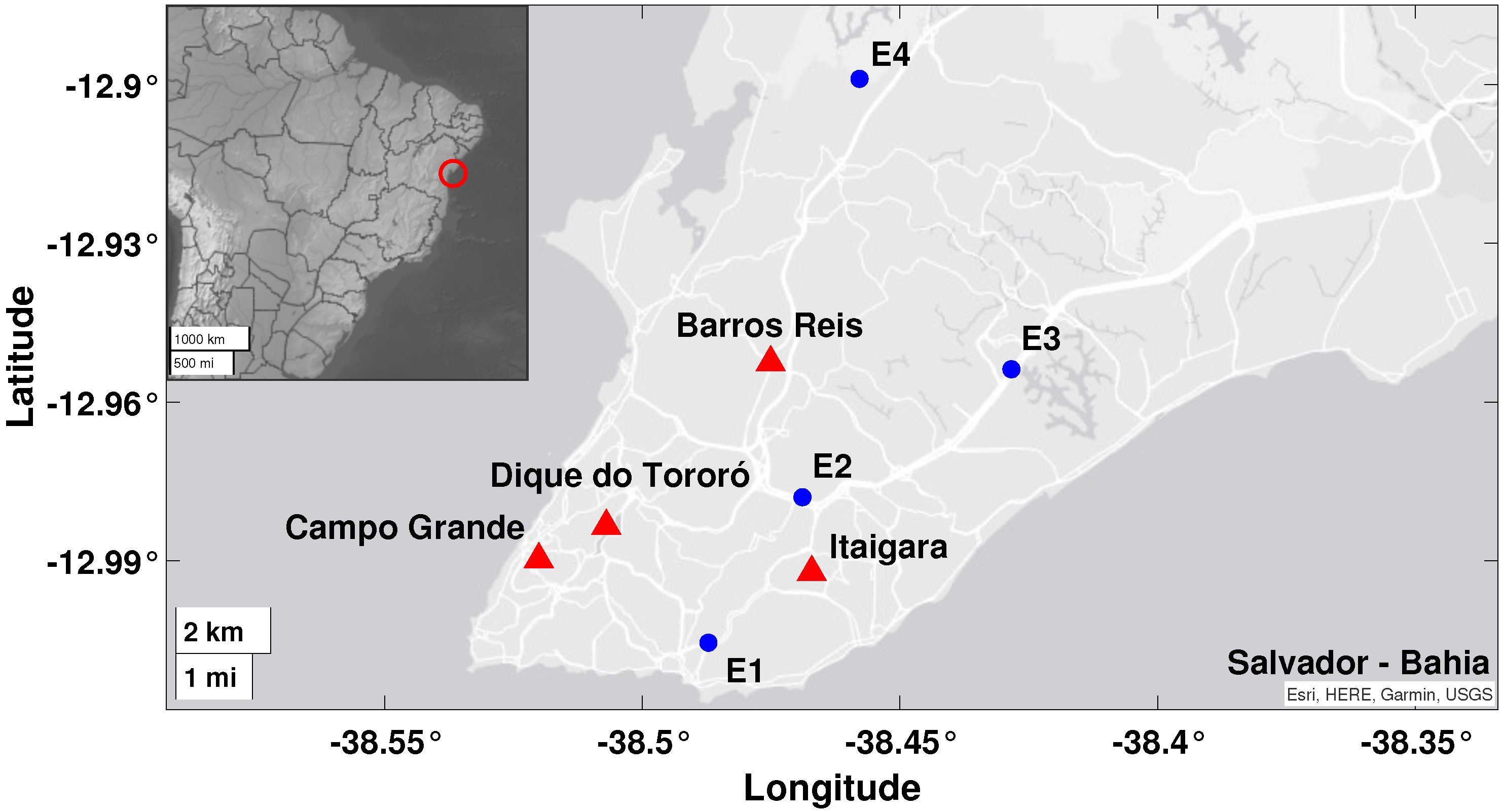
Article

Analysis of Atmospheric Pollutant Data Using Self-Organizing Maps

by
Emanoel L. R. Costa
1,†,
Taiane Braga
2,†,
Leonardo A. Dias
3,†,
Édler L. de Albuquerque
4,*,† and
Marcelo A. C. Fernandes
1,5,*,†
1
Laboratory of Machine Learning and Intelligent Instrumentation, Federal University of Rio Grande do Norte, Natal 59078-970, RN, Brazil
2
Federal Institute of Education, Science, and Technology of Bahia, Salvador 40301-015, BA, Brazil
3
Centre for Cyber Security and Privacy, School of Computer Science, University of Birmingham, Birmingham B15 2TT, UK
4
Department of Industrial Processes and Chemical Engineering, Federal Institute of Education, Science and Technology of Bahia, Salvador 40301-015, BA, Brazil
5
Department of Computer Engineering and Automation, Federal University of Rio Grande do Norte, Natal 59078-970, RN, Brazil
*
Authors to whom correspondence should be addressed.
These authors contributed equally to this work.
Sustainability 2022, 14(16), 10369; https://doi.org/10.3390/su141610369
Submission received: 12 July 2022 / Revised: 16 August 2022 / Accepted: 17 August 2022 / Published: 20 August 2022
(This article belongs to the Special Issue Air Quality Characterisation and Modelling)

Abstract

:
Atmospheric pollution is a critical issue in our society due to the continuous development of countries. Therefore, studies concerning atmospheric pollutants using multivariate statistical methods are widely available in the literature. Furthermore, machine learning has proved a good alternative, providing techniques capable of dealing with problems of great complexity, such as pollution. Therefore, this work used the Self-Organizing Map (SOM) algorithm to explore and analyze atmospheric pollutants data from four air quality monitoring stations in Salvador-Bahia. The maps generated by the SOM allow identifying patterns between the air quality pollutants (CO, NO, NO2, SO2, PM10 and O3) and meteorological parameters (environment temperature, relative humidity, wind velocity and standard deviation of wind direction) and also observing the correlations among them. For example, the clusters obtained with the SOM pointed to characteristics of the monitoring stations’ data samples, such as the quantity and distribution of pollution concentration. Therefore, by analyzing the correlations presented by the SOM, it was possible to estimate the effect of the pollutants and their possible emission sources.

1. Introduction

Air pollution is one of the crucial challenges of modern society. In recent years, pollution caused by industrial, vehicular, and toxic-chemical emission sources has increased significantly. This increase can be seen mainly in low- and middle-income countries, also called developing countries [1]. Despite the continuous pollution growth, awareness and pollution control programs are limited and receive little attention and financial resources from governments, international agencies, and philanthropic donors [1].
In addition, effectively managing regulations for controlling air pollution requires considerable knowledge about the costs and benefits. Currently, the primary efforts for measuring pollutants aim to avoid possible harm to people’s health, such as respiratory or cardiovascular diseases that can result in hospitalizations and even death, usually affecting vulnerable groups of the population [2].
Complex mixtures of solid particles and gaseous pollutants contribute to air pollution. Among these are priority pollutants, commonly regulated by law and categorized as primary and secondary. The primary pollutants are substances that can be released directly into the atmosphere, while the secondary pollutants are substances derivated from the primary ones through photochemical reactions in the troposphere [3]. Regarding the gaseous pollutants, to be particulary mentioned are sulfur dioxide (SO2), nitrogen dioxide (NO2), carbon monoxide (CO), volatile organic compounds (VOCs), solid materials or liquids suspended in the atmosphere due to their small size (called particulate matter (PM)), and the ozone (O3). The ozone is one of the major photochemical pollutants formed in the atmosphere by the reaction of nitrogen oxides (NOx) and hydrocarbons such as VOCs in the presence of sunlight, similarly to particulate sulfate and nitrate aerosols created from SO2 and NOx [3].
The dispersion of atmospheric pollutants results from different elements such as temperature, relative humidity, atmospheric pressure, wind direction and speed, as well as topography [4]. Consequently, the complexity of analyzing and identifying pollutants and their primary sources in large-scale areas increases, which leads to the problem of positioning monitoring stations for data collection.
There are several emission sources of air pollutants, and a single source can emit several pollutants. For instance, the composition of fossil fuels used in motor vehicles can emit different pollutants during combustion and evaporation, or by the wear of tires and roads where vehicles run. Due to the increasing number of private vehicles, their emissions have become a dominant source of CO, CO2, VOCs, NOx and PM. Meanwhile, industrial processes normally include pollutants such as CO, PM, NOx, and SO2 [4,5,6].
Thus, monitoring the concentration of pollutants in the environment at specific points is essential. Identifying the main components enables understanding of the current condition of air pollution, variations, correlations, and possible emission sources, which leads to the development of public policies to raise awareness and reduce pollutants. Therefore, many researchers have proposed the analysis of environmental data mainly using multivariate statistical techniques [4,7,8].
Multivariate statistical methods such as correlation or cluster analysis [9,10,11,12,13], and principal component analysis [7,14,15] are commonly applied in various studies to identify the correlation among parameters that can influence air quality. Large databases that carry various information about air pollution require techniques to extract and identify characteristics inherent to the analyzed data.
In this context, machine learning has proved to be a great alternative to the traditional methods used [16,17]. A well-known algorithm that belongs to the group of unsupervised learning algorithms is self-organizing maps (SOM) [18]. The SOM supports data dimensionality reduction and clustering. In addition, the SOM does not need to make assumptions about the parameters’ distribution, as it is capable of dealing with non-linear problems of great complexity and dimension and is effective in using noisy data [19].
The SOM algorithm is adopted in many applications to analyze data from atmospheric pollutants. For example, in Ref. [20], the SOM is used to analyze data regarding air quality. In Ref. [21], the SOM is used to identify the level of pollution during foundry and land mining. The study carried out in [22] used the SOM to highlight the impact on air quality caused by the circulation of different air types, which alters the concentration of pollutants in the atmosphere. For this purpose, it is essential to identify suitable placements for positioning monitoring stations, as shown in [23]. Finally, the SOM has also been used to obtain particulate-matter characteristics in the atmosphere by evaluating its concentration in both internal and external exposure and connecting them to human activities. According to [24], the SOM can also function as a pollution identifier by defining limits to classify regions with low or high concentrations of a specific pollutant, such as ozone, enabling the evaluation of pollution zones.
Therefore, this work proposes an SOM implementation to study and analyze atmospheric pollutants to identify their patterns and characteristics. The main contributions are:
  • A machine-learning-based approach for analyzing the air quality of Salvador monitoring stations, using the Government of Bahia State database—to the best of our knowledge, this work is the first to analyze this data using machine-learning algorithms.
  • We discuss the common factors among meteorological parameters and pollutants and their clusters’ impact on each monitoring station.

2. Methodology

2.1. Case Study

Salvador city (State of Bahia) has a territorial area of 693.453 km2 and a population of 2,675,656 people. Located in the northeastern region of Brazil, it has an urban core and rugged topography formed by several columns and valleys, with a rainy tropical climate with no dry season and an average annual temperature of 25 °C.
The Government of Bahia State, through CETREL S. A., the company that operated the air monitoring stations from 2011 to 2016, provided the air quality database for this work. It contains the air quality data of a monitoring network constituted of eight stations. Nonetheless, we used data from four stations: Barros Reis (BR), Campo Grande (CG), Dique do Tororó (DT), and Itaigara (IT), due to their inherent characteristics. Figure 1 illustrates the stations’ distribution in Salvador and highlights the four chosen. It is important to mention that this is the first air quality monitoring network ever installed in the city of Salvador. Therefore, this work portrays the first analysis of the pollutant and meteorological parameters in the database provided.

2.2. Dataset

The dataset contains the hourly average of twelve features related to meteorological parameters and pollutants concentration. The meteorological parameters are wind speed (WS), ambient temperature (TEMP), relative air humidity (RH), the standard deviation of wind direction (STWD), rainfall, and wind direction. Meanwhile, the pollutants are SO2, CO, O3, particulate matter whose aerodynamic diameter is less than 10 μ m (PM10) and the oxides of nitrogen NO2 and NO. We removed the rainfall and wind direction variables due to the small amount of data available; thus, only ten features were used in our analysis.
We performed a data preprocessing step by removing the null lines, the measurement errors (identified by a specific terminology), and the outliers to improve the quality of the analysis. The outliers were removed by investigating the data dispersion and symmetry and, subsequently, using the quartile separatrix measure [25] to divide the dataset into three quartiles: Q 1 , Q 2 and Q 3 . Finally, based on the interquartile range ( A I Q ) [25], outliers with value greater than Q 3 + 3 × A I Q and less than Q 1 3 × A I Q , were removed from the database. We kept outliers with values greater than Q 3 + 1.5 × A I Q and less than Q 1 1.5 × A I Q to avoid a large reduction in the dataset. Table 1 presents the number of data samples for each monitoring station considered in our analysis and their period of operation.
In the meantime, Table 2, Table 3, Table 4 and Table 5 present the dataset for the Barros Reis (BR), Campo Grande (CG), Dique do Tororó (DT), and Itaigara (IT) stations, respectively. As can be observed, all pollutants and atmospheric data are shown after the preprocessing step for each station in a concentration of pollutants in parts per billion (ppb).
As can be observed, the BR station presents a higher concentration of SO2, CO, and PM10. The SO2 has a maximum of 3.20 ppb and an average of 0.45 ppb due to the burning of fuels with sulfur. Meanwhile, the CO has a maximum of 2180 ppb and an average of 601.6 ppb, produced by burning organic fuels. The PM10 has an average of 40.10 ppb, almost double the value of other stations; it is a solid or liquid material that remains suspended in the atmosphere that can cause a significant impact on human health.
The CG station also has a high level of CO, with a maximum of 1830 ppb and an average of 396.6 ppb. Regarding the presence of nitrogen oxides (NO and NO2), the CG and DT stations present higher average and maximum concentrations due to the combustion processes and atmospheric chemical reactions. Concerning the O3, a secondary pollutant formed in the atmosphere indicating the presence of photochemical oxidants, it has its higher concentrations recorded at the DT and IT stations.
Therefore, the SO2, CO, and NO pollutants present the most significant variations in concentration. These pollutants are mainly generated from the burning of fossil fuels. Hence, the station location and the intensity of the vehicle’s traffic around its region can lead to different concentration records at certain times of the day. The datasets comprise 24 h of daily data collection.
All stations show similar measured values regarding the meteorological parameters, except for wind speed which has a high average at BR and IT stations, and the standard deviation of wind direction at CG. Note that the values were rescaled from 0 to 1 to improve the SOM results. In addition, this work performed the z-score normalization and logarithmic transformation, obtaining data with null mean and unit variance and reducing the data scale, respectively.

2.3. Self-Organizing Maps (SOM)

The Self-Organizing Map (SOM) is a neural network model widely applied to data dimensionality reduction and clustering [18,26]. The map consists of M neurons commonly arranged in a two-dimensional array representing the incoming data by shifting the neurons’ position towards it. The maps’ topology can be rectangular, hexagonal, or square, among others [18].
The N-dimensional input data sample can be characterized as
x = [ x 1 , x 2 , , x N ] .
Accordingly, each i-th neuron in the map is represented by a N-dimensional vector of weights expressed as
w i = [ w i 1 , w i 2 , , w i N ] .
Therefore, the topology of a two-dimensional map with M neurons can be expressed as M h × M v , where M h is the number of neurons in the horizontal and M v is the number of neurons vertically; thus, M = M h × M v .
The SOM algorithm iteratively molds the neurons’ map to the input data topological form, based on a similarity metric, according to the following steps [18]:
  • Randomly initialize the M neurons’ weight vectors.
  • Calculate the distance of each p-th input data sample, x ( p ) , to all M neurons.
  • Define the winning neuron, also known as best matching unit (BMU); it is the j-th nearest neuron to the input data defined based on a distance metric as follows:
    j = arg min i | | x ( p ) w i | | , i = 1 , 2 , , M .
  • Update the BMU neuron and its neighboring neurons’ weights according to following
    w i ( t + 1 ) = w i ( t ) + η ( t ) h i , j ( t ) ( x ( p ) w i )
    where η ( t ) is the learning rate (ranging from 0 to 1) and h i , j ( t ) represents the BMU neighborhood function at the t-th iteration. The neighborhood function is described as
    h i , j ( t ) = exp d i , j 2 2 σ 2 ( t )
    where d i , j 2 is the distance from the i-th neuron to the BMU (j-th neuron) and σ 2 ( t ) is the neighboring function size at the t-th iteration.
  • Repeat steps 2, 3 and 4 until the maximum number of iterations is reached, represented here by T.
The number of iterations must be enough to process the dataset samples several times; thus, T = b × P , where b is the repetition number that every set of P samples is presented to the SOM. Moreover, increasing the iteration number (t) decreases the radius of the neighborhood function, σ 2 ( t ) . Consequently, the number of neurons nearby the BMU to be updated is reduced, strengthening their connection and similarities. After training the network, each p-th entry x ( p ) is associated with a specific BMU in the output layer, and entries that share similar patterns will be associated with the same BMU or its neighbors, which can be understood as a grouping in the SOM.
We applied the SOM to each monitoring station shown in Table 1. Each p-th sample in the dataset has N = 10 dimensions, 6 regarding atmospheric pollutants (SO2, CO, O3, PM10, NO, and NO2) and 4 concerning meteorological parameters (WS, TEMP, RH, and STWD). Therefore, the SOM enables analyzing the influence and characteristics of these variables.

2.4. SOM Parameters

The map size is the first parameter to be defined. For this purpose, it is necessary to determine the number of neurons to be used during training; in addition, avoiding a large or small number of neurons is vital to prevent problems such as non-identification of characteristics and overfitting [27]. Commonly, the number of neurons can be determined using the following heuristic equation
M 5 P
where P is the number of input data samples [27].
Subsequently, the map topology ( M h × M v ) was defined according to quality measures commonly used for the SOM network, the quantization error (QE) and topographic error (TE) [28,29]. For each station, different values of M h and M v were tested, in which M h × M v = M (Equation (6)). Finally, to analyze the results, three different types of normalization were applied to the data: z-score, min–max, and logarithmic.
Hence, all tests were performed with b = 500 , a hexagonal topology, and the training algorithm was applied in two steps. Firstly, the learning rate and neighborhood function were initialized as η ( 0 ) = 0.5 and σ 2 ( 0 ) = M h 2 , respectively, and decreased over iterations. Secondly, these values were fixed as η = 0.05 and σ 2 = 1 . Table 6, Table 7, Table 8 and Table 9 present the quality measures obtained for each test.
Considering both QE and TE measures, the lowest values were obtained using min–max normalization. Thus, M h and M v were chosen according to the best result, being highlighted in each table.

3. Results

3.1. U-Matrix, Components Plane and Parameter Similarity

The SOM output can be represented by a unified distance matrix (U-matrix) and a component plane, both illustrated in Figure 2. The U-matrix provides a visualization of the relative distance between neurons in the map, which is evidenced through a color scale, and highlights the calculated distance between the adjacent neurons [18]. The closer the color approaches a dark blue in the U-matrix, the closer these neurons are, i.e., they have a more significant similarity. On the other hand, the closer the color approaches a dark red, the greater the distance between the neurons and their dissimilarity. In general, this form of representation allows us to consider that neurons with smaller distances form a cluster. In contrast, neurons with high distances can be considered as boundaries of a cluster.
The component plane shows the values of the weight vectors of each neuron through a color code, where the blue and red colors correspond to low and high values, respectively. This representation allows the recognition of parameter dependencies by comparing the patterns of each plane. The color gradient of a plane represents the parameters’ value (component) for the analyzed samples. Each neuron is assigned a color according to the parameter value in that neuron; thus, it can be said that two or more parameters are related based on a comparison of their color gradients. A coherent gradient indicates a positive correlation, while an inverse gradient a negative correlation.

3.2. Itaigara Station

Analyzing the component planes in Figure 2, it is possible to note that the relative humidity (RH) and temperature (TEMP) planes display inverse gradients, indicating a negative correlation between these parameters—something already expected given their characteristics. For CO, NO, and NO2 pollutants, their weight vectors present a dark red color on the left side of the components’ plane, with a higher concentration of high values at the top left side; hence evidencing a certain similarity between them. These pollutants are generated by combustion, and incomplete burning of organic fuels, which are very common in cities with a large circulation of vehicles (the leading emitter) [5].
The O3 pollutant can be formed by the reaction of nitrogen oxides with VOCs. However, it presents a different pattern than NO2, which contributes to the formation of photochemical oxidants such as O3. As can be seen in the O3 component plane, its high-value region is concentrated on the right side, similar to the wind speed component plane. Therefore, it can be said that the O3 presence at the Itaigara Station probably came from another region carried by the wind, as it has a low concentration near traffic routes and is generated by photochemical reactions.
The PM10 showed a different pattern than the other pollutants. Its main concentration region, with high weight vector values, is in the upper part of the plane. Since its emission sources are diverse, such as vehicles, biomass burning, industries, and dust resuspension, it is difficult to identify the major contributor pollutant. However, its formation can also be carried out in the atmosphere through VOCs, SO2, and nitrogen oxides.
The most distinct pattern presented was by SO2, with high values and concentration in the lower left part, it does not resemble any other component plane. This pollutant is released mainly by heavy vehicles burning diesel oil in urban areas.
An SOM arranges similar patterns in the same neighborhood region, clustering the network’s output. Hence, an investigation into the clustering of samples provides important information about the data.
The U-matrix in Figure 2 illustrates how close or far the neurons are, showing their clusters. However, the cluster boundaries are not clearly represented, making it challenging to identify them. One of the methods for choosing the appropriate number of clusters is the so-called Davies–Bouldin index [30], an evaluation measure commonly used in SOM networks for validating clusters [31,32].

3.2.1. Sample Grouping with the SOM Algorithm

For the Davies–Bouldin index, the lowest value found indicates the best number of clusters for the analyzed problem. Thus, an experiment was conducted by varying the number of clusters from two to eight and observing the obtained values. The best result was achieved for a total of four clusters.
Aftwards, a hierarchical analysis was performed to define the neurons belonging to the four clusters. For this purpose, the Euclidean distance was used as the similarity metric and the Ward neuron linking criterion, illustrated by the dendrogram shown in Figure 3. A dendrogram threshold value is defined for that to which cluster each neuron belongs (horizontal line in Figure 3).
In addition, based on the hierarchical analysis, the SOM neurons were classified in four clusters, as shown in Figure 4. Therefore, the samples assigned to each cluster and its neurons present the characteristics of the distribution of pollutants and meteorological parameters. Table 10 shows the mean value of samples for each parameter and cluster.
According to Table 10, cluster 1 samples exhibit, in general, a low concentration of air pollutants, except for O3 and PM10, which have the highest average concentration. In addition, cluster 1 presents a wind speed and temperature considerably higher, and lower relative humidity. In total, about 34 % of the data was assigned to cluster 1, thus sharing those characteristics.
Cluster 2, presented in Table 10, shows the lowest concentrations of SO2, CO, PM10, and NO pollutants, with intermediate values of O3, and NO2. It also presents the lowest average wind speed, intermediate temperature, and high relative humidity. In addition, cluster 2 is composed of 29 % of the data, characterized by a low concentration of pollutants.
The highest concentrations of CO, PM10, NO, and NO2 are found in cluster 3, as can be observed in Table 10. In contrast, SO2 and O3 show low values (with O3 having the lowest total average among all clusters). The wind speed, temperature, and relative humidity have intermediate values. A total of 24 % of the data was assigned to cluster 3, characterized by high pollutant concentration values.
Finally, cluster 4 is mainly characterized by the high concentration of the SO2 pollutant compared to the others. The other pollutants present intermediate concentration values, as well as wind speed, temperature, and relative humidity. In addition, cluster 4 has the lower amount of samples; a total of 2027 ( 13 % ) were assigned here.

3.2.2. Parameter Correlation

The component planes allow an initial and preliminary analysis of parameters through their visual gradients which, in a certain way, can turn out to be subjective and discretionary. Thus, to carry out a more objective and effective analysis of the results, a correlation analysis was applied between the component planes seen in Figure 2. Figure 5 shows the similarity between the planes (parameters) using the Ward criterion and the Pearson correlation coefficient, r.
As can be observed in Figure 5, two main branches are seen in the correlation analysis. The first branch, on the left of the figure, includes all the pollutants studied but O3, whose origin is exclusively photochemical. Hence, O3 is clustered with the wind speed and temperature.
The NO, NO2, and CO pollutants have a substantial similarity, probably due to a similar emission source such as vehicular, given the station allocation and the monitoring region. Those pollutants are correlated to PM10, which also has a vehicular origin. In addition, the PM10 is connected to STWD, showing that intensive vertical turbulence (atmospheric instability), which is characterized by high STWD values, increases the PM10 concentration. Thus, it can be said that the wind movement is dragging out PM10 from other areas or causing the resuspension of particulate material at Itaigara station. In addition to vehicle influence, the particulate matter may also be dispersed by the existing vehicle movement, the wear of traffic lanes, and the vehicles’ brake pads.
The similarity between RH and SO2 shows the influence of RH on the formation or decomposition process of molecules during the heterogeneous procedure (liquid phase). In particular, the SO2 can react with the air humidity and other oxidants in the atmosphere to form sulfuric acid H2SO4 and ammonium sulfate [33].
Meteorological parameters, such as wind speed, considerably influence the O3 pollutant [24]. Given the similarity between O3, the wind speed, and temperature (Figure 5), we consider that O3 is not generated at the monitoring station site but instead transported by winds along with other pollutants such as VOCs. The temperature may also be responsible, since high temperatures result from the increase in the speed of chemical processes, generating ozone in the region.

3.3. Barros Reis Station

In the BR station component planes (Figure 6), the weight vectors for the PM10, CO, NO, and NO2 are displayed similarly across the map. The concentration of high values is on the upper left side, with average values in the nearby regions. The low values are located mainly in the lower right region of the map. All these pollutants can be formed from combustion processes, which shows the similarity obtained and, in particular, if they have a common source.
Unlike the pollutants discussed above, the O3 component plane has its highest concentration at the bottom right of the map. O3 is a secondary pollutant, i.e., its formation depends on atmosphere reactions from other pollutants, such as NO2. Still, its plane does not resemble the planes of primary pollutants. Similarly, PM10 is also a secondary pollutant but is formed by SO2, and no similarity is seen in their plane. However, PM10 can also be obtained from VOCs and nitrogen oxides, showing a relationship between their planes.
The SO2 plane displays a unique pattern, with its highest values concentrated in the upper right region of the map, showing no similarity with the other pollutants. The component planes referring to meteorological parameters showed different distributions, with a negative correlation between TEMP and RH. At the same time, the high WS values are concentrated in the upper central region, and STWD with values dispersed throughout the map.

3.3.1. Sample Grouping with the SOM Algorithm

Figure 6 presents the clusters through the U-matrix, representing the neurons with their distance to adjacent neurons. The cluster number was defined with the Davies–Bouldin index by varying it from two to eight, reaching the best result for three clusters.
Subsequently, a hierarchical analysis was performed to define the neurons belonging to the three clusters. Thereupon, the Ward criterion and the Euclidean distance were used as similarity metrics. Figure 7 displays the dendrogram obtained with the threshold value used for segregation. Meanwhile, Figure 8 shows how the clusters were arranged on the map.
The samples are linked to a particular neuron belonging to one of the three clusters, allowing the analysis of the sample’s distribution regarding the clusters.
Table 11 shows the average values of every parameter according to the cluster. As can be seen, cluster 1 represents the samples with the lowest pollutant concentration, except for O3 which has a median value among the others. Meteorological parameters such as wind speed, temperature, and relative humidity also have low values. In total, the cluster has 10,599 samples with these characteristics, corresponding to 49.16 % of the station data.
In the meantime, cluster 2 exhibits the highest concentration of pollutants, displaying a considerable difference from the values of other clusters except for O3, which has the lowest average value obtained. Similar to cluster 1, the wind speed, temperature, and relative humidity also have low values. Cluster 2 has 4183 samples, equivalent to 19.40 % of the data.
Finally, the samples assigned to cluster 3 have an intermediate value of pollutants concentration, with average values between the clusters 1 and 2 range, except for O3 which has the highest average concentration recorded. In addition, cluster 3 has 31.44 % of the station data with the highest wind speed and the lowest relative humidity.

3.3.2. Parameter Correlation

The component planes, shown in Figure 6, present the correlation between parameters. Meanwhile, Figure 9 presents the parameters similarity obtained using the Ward linking method and the Pearson correlation coefficient.
As shown in Figure 9, there is a substantial similarity between CO and NO pollutants. Given the BR station characteristics (located in between two avenues), it can be said that motor vehicles are the primary emission source of those pollutants. Likewise, the NO2 and PM10 pollutants are also emitted by combustion in vehicles; in addition, they can be formed secondarily by photochemical processes. Regarding SO2, it can be said that the primary emission source is the burning process of fuels, such as diesel and gasoline, from heavy vehicles such as trucks, buses, microbuses, and light vehicles.
Unlike other pollutants, the O3 showed a clear relationship with meteorological parameters such as wind speed and temperature, similar to the Itaigara station. Nonetheless, this relationship with meteorological parameters is not strong as in other stations.
The STWD indicates the local atmospheric stability. Its inverse relationship with RH can be related to the regions’ water molecules’ dissipation. Hence, the data regarding pressure and heat could improve the analysis precision by demonstrating the influence of the wind direction. The RH and STWD present a negative relationship with the other pollutants, consequently leading to the non-contribution or reduction in the present concentrations.

3.4. Campo Grande Station

Figure 10 illustrates the component planes for the CG station. Concerning the planes of nitrogen oxide, a significant similarity between NO2 and CO can be observed, with high values concentrated in the central part of the map. The NO plane is also similar to the CO and NO2, but the high values are concentrated in the region to the right, while median values are concentrated in the map center. The emission source of these pollutants is fuel combustion, especially from vehicles.
The SO2 has high values concentrated in the lower right region of the map. The PM10, on the other hand, did not show significant pattern similarities with other planes, having a higher concentration in the upper part of the map and moderate concentration in the lower part, equivalent to small regions of the SO2 and NO2 planes. Likewise, the O3 pollutant also shows no similarity with other component planes. Despite its formation, resulting from the reaction between NO2 and VOCs, its concentration of high values is located at the map edges, having similarities with the concentration regions of high values of meteorological parameters, such as WS, TEMP, RH, and STWD.

3.4.1. Sample Grouping with the SOM Algorithm

To identify the CG station clusters through the U-matrix, illustrated in Figure 10, the Davies–Bouldin was used and the cluster number varied from two to eight. The best result was obtained for five clusters. Aftward, the neurons belonging to each cluster were obtained according to a hierarchical analysis defined based on the Ward method and Euclidean distance. Figure 11 shows the resulting dendrogram and the segregation threshold. Meanwhile, Figure 12 displays the neurons distribution regarding the clusters.
Each CG station dataset sample was integrated into the cluster with the neuron it most resembles. Thus, an analysis was performed regarding the samples’ distribution by cluster based on the average values of parameters, as shown in Table 12.
According to Table 12, cluster 1 has the lowest average values of concentration for the SO2, CO, NO, and NO2 pollutants, while the PM10 and O3 show intermediate values. Moreover, the wind speed and temperature are the lowest of all. Cluster 1 consists of 6640 data samples, equivalent to 27.04% of the dataset.
Cluster 2 also presents low average values of the concentrations of the pollutants, with values slightly higher than those obtained in cluster 1, except for the O3 pollutant, which has a higher concentration average. Similar behavior can be seen for the meteorological parameters except for the wind speed, which shows the highest average among all clusters. In total, 16.96 % of the data was assigned to cluster 2.
The samples assigned to cluster 3 present intermediate values for all pollutants concentration and meteorological parameters, where the temperature has the highest average and the relative humidity the lowest. This cluster has 25.34 % of the data.
The highest concentrations of CO, PM10, NO, and NO2 are found in cluster 4, with an intermediate concentration of SO2 and the lowest concentration of O3. Meanwhile, all meteorological parameters showed intermediate values compared to other clusters. Cluster 4 has a total of 17.22 % of the data.
Meantime, cluster 5 stands out with the highest average concentration of the SO2 pollutant. The other pollutants, as well as the meteorological parameters, present intermediate average values. In total, 7.44 % of the data was assigned to cluster 5.

3.4.2. Parameter Correlation

The hierarchical representation for the CG station was obtained with the Ward method and the Pearson correlation coefficient. Figure 13 presents the parameters’ correlation obtained.
First of all, the similarity between CO, NO, and NO2 pollutants can be seen. These pollutants are emitted in urban areas mainly by motor vehicles, and their similarity validates the idea of a potential common emission source. The temperature is also similar to those three pollutants as it contributes to chemical processes that form them—for example, the NO2 results from the sunlight action on NO. Thus, the temperature can impact the amount of those pollutants present in every season.
The PM10 is a primary and secondary pollutant, and it is correlated to SO2. Thus, its atmospheric formation can be linked to gases turning into particles due to chemical reactions in the air, such as sulfur dioxide. The SO2 is generated from the burning of fuels with sulfur in its composition, such as diesel oil or industrial fuel oil, and it appears to be related to the PM10 due to motor vehicle emissions, among other processes.
The photochemical oxidant, O3, has a certain correlation with the wind speed, but with a much lower similarity than that presented by the Itaigara station. In addition, there is no apparent relationship with the temperature. The RH has a negative relationship with O3 and wind speed, which may be a consequence of solar radiation; low RH concentrations are related to a high solar incidence and, therefore, a greater disposition to the O3 formation.

3.5. Dique do Tororó Station

The SOM network component planes for the DT station are shown in Figure 14. The pollutants that are mainly emitted by combustion processes, such as CO, NO, NO2, and PM10 showed similar distribution patterns of values, with the highest concentration from the left side to the upper left side of the map. In contrast, the PM10 has higher values at the bottom of the map, similar to the temperature and wind speed.
As in the other stations, the SO2 showed a different pattern from the other pollutants, with regions of high values concentration at the edges of the map. However, one of the high-concentration edges slightly coincides with those of the CO, NO, and NO2. Lastly, the O3 displays high values at the lower right region of the map, with a similar distribution to the wind speed plane. The other planes, such as relative humidity and STWD (which can influence the concentration of pollutants), showed patterns with well-defined regions at the top of the map.

3.5.1. Sample Grouping with the SOM Algorithm

The map neurons, represented by their respective distances to adjacent neurons in the U-matrix (Figure 14), were used to visualize and determine the clusters. For this purpose, the Davies–Bouldin index was used, and the number of clusters varied from two to eight, resulting in the best amount with three clusters. Again, hierarchical analysis was carried out using the Ward criterion and Euclidean distance. Figure 15 illustrates the dendrogram, and Figure 16 the segregation borders of the map.
Each cluster was assigned a certain number of samples according to their characteristics. Table 13 presents the concentration averages of each pollutant according to the cluster.
As can be seen in Table 13, cluster 1 represents the samples with the highest mean value of O3 and intermediate values of the other pollutants (SO2, CO, NO, NO2, and PM10). The highest concentration value is the wind speed, while relative humidity and STWD are the lowest. Cluster 1 has 26,101 samples sharing its characteristics, equivalent to 62.09 % of the station data.
The pollutants in cluster 2 had the highest average concentration, except for O3 which showed the lowest concentration among all clusters. The wind speed presents low values, and the temperature parameter is the highest. In total, 17.87 % of data constitutes this cluster.
Finally, the pollutants in cluster 3, that is, CO, NO, NO2, and PM10, had the lowest average concentrations, with SO2 and O3 showing intermediate values. The temperature and wind speed parameters have the lowest values found and the relative humidity the highest. Cluster 3 represents 20.04 % of the station data with 8425 samples.

3.5.2. Parameter Correlation

The DT station component planes, shown in Figure 14, presents the parameters correlation. Meanwhile, Figure 17 illustrates the parameter similarity obtained through the Ward criterion and the Pearson correlation coefficient.
As can be seen in Figure 17, the CO, NO, and NO2 pollutants have the most significant similarity, a characteristic also observed for other stations. All stations are located in urban centers with a large flow of vehicles, leading to the possibility of a common emission source of these pollutants, mainly coming from the local vehicular fleet. The PM10 also showed a certain similarity with those pollutants, indicating a possible emission from fuel burning. The temperature parameter at the DT is also related to the mentioned pollutants, different from other stations where it is associated with O3. In addition, the temperature can contribute to NO2 formation and PM10 in secondary processes.
Like Barros Reis station, the RH and the STWD at the DT station are somewhat similar but with a positive coefficient. The RH and STWD can be influenced by atmospheric parameters such as pressure and heat and, consequently, the wind conditions and water particles.
The SO2, different from the Itaigara station, is not correlated to either the PM10 or RH, as it is probably being generated by an independent source and not reacting to other pollutants.
Given that O3 is a secondary pollutant, it was only correlated with wind speed, with no apparent similarity with temperature or nitrogen oxides. Therefore, its concentration at the DT station may be transported by the wind accompanied by other pollutants.

4. Discussion

The SOM implementation presented in the previous sections identifies the correlation among different air quality parameters for many monitoring stations. The SOM component planes provide a visual representation of the similarities between pollutants and meteorological parameters, simplifying their analysis and highlighting peculiarities.
Usually, the CO, NO, and NO2 pollutants were related, showing higher similarities. On the other hand, the meteorological parameters differed from PM10 and SO2. The RH and STWD parameters at Barros Reis station showed a negative correlation, unlike at Dique de Tororo station, where a positive correlation was presented. At Itaigara station, the influence of atmospheric stability was identified through the relationship between STWD and PM10. Meanwhile, Campo grande station shows some degree of similarity between PM10 and SO2. These relations are essential to identify the influence of meteorology on air-pollutants concentrations and information employed to create strategies for mitigating air-pollution critical episodes.
Unlike other pollutants, the O3 presents a more significant link with meteorological parameters such as WS, as seen at Itaigara, Dique do Tororó and Campo grande stations. Thus, we can infer that the wind is mainly responsible for the transport of O3. In addition, the correlation of the TEMP, WS, and O3 parameters at Barros Reis and Itaigara stations indicates an increase in O3 resulting from chemical processes, probably due to the influence of solar radiation.
The data of Dique do Tororo and Barros Reis stations were grouped only into three clusters, with their cluster 1 emphasizing a large number of samples with higher concentrations of O3. In contrast, the other clusters present a sample distribution with intermediate to high concentrations for the CO, NO, NO2, PM10, and SO2 pollutants. Meanwhile, the Itaigara station has four clusters, with one mainly characterized by the SO2 pollutant; the remaining clusters are defined by higher concentrations of CO, NO, NO2, PM10, and O3. Similar to Itaigara, the Campo Grande station has one cluster (out of five) where SO2 is predominant, while the other clusters display low and high concentrations.
Commonly, studies about atmospheric pollutants rely on methods such as principal component analysis (PCA) and hierarchical analysis to define clusters based on similarity. For example, the studies carried out by [8,34] describe the clusters’ characteristics according to the percentage of their main components’ variance, thus, indicating which variables have more significance for their definition. Meanwhile, by applying a hierarchical classification on the SOM neurons, we can obtain the variables’ concentration value and influence on defining each cluster.
In the meantime, in [13,35], the number of clusters is fixed for all monitoring stations, and the k-nearest neighbors provide a relationship between the defined clusters of each station. However, the SOM also allows an individual characteristic analysis of each pollutant, like in [35].
Thereby, the SOM enables finding similarities and estimating the link between parameters more deeply. As described in this work, the SOM can obtain data patterns and cluster characteristics and demonstrate the parameters’ influence, which is not trivial in other techniques. Additionally, it can also deal with the non-linearity complexity of air pollution data [36], simplifying the analysis process and increasing its precision; this shows the advantage of using a machine-learning-based approach compared to traditional methods.

5. Conclusions

We implemented an SOM to analyze the air-quality data of four stations in the monitoring network of Salvador, Brazil. A detailed discussion regarding pollutants and their correlation with meteorological parameters is provided, assisting in estimating possible common emission sources and the influence of meteorological parameters. The latter permits the establishment of relations between meteorology and pollutants concentration, which is vital for developing, for example, alert systems to identify critical episodes of air pollution or for assisting in developing strategies to improve air quality.
The SOM outputs enabled the identification of data particularities concerning the parameters analyzed. For example, the data samples’ concentration of Dique do Tororo and Barros Reis stations showed a cluster with a high concentration of O3. In contrast, the other clusters presented well-defined contributions of remaining pollutants. The Itaigara and Campo Grande stations presented a more detailed definition regarding the clusters of (1) CO, NO, NO2; (2) MP10; (3) O3; and (4) SO2. Thus, the SOM also allows an analysis of the particularities of each cluster.
The results showed that the SOM could identify characteristics, describe similarities, recognize patterns, and define clusters of air-pollution problems. Unlike traditional methods, the SOM proved to be a good tool for studying atmospheric pollutants, providing several aspects that can contribute to and improve discussions in this area. To the best of our knowledge, this is the first study to analyze Salvador’s air-quality monitoring database. Therefore, the tool developed and the results presented and discussed here can assist further studies and aid in the development of public policies for pollution management.

Author Contributions

All the authors have contributed in various degrees to ensure the quality of this work (e.g., E.L.R.C., T.B., L.A.D., É.L.d.A. and M.A.C.F. conceived the idea and experiments; E.L.R.C., T.B., L.A.D., É.L.d.A. and M.A.C.F. designed and performed the experiments; E.L.R.C., T.B., L.A.D., É.L.d.A. and M.A.C.F. analyzed the data; E.L.R.C., T.B., L.A.D., É.L.d.A. and M.A.C.F. wrote the paper. É.L.d.A. and M.A.C.F. coordinated the project). All authors have read and agreed to the published version of the manuscript.

Funding

This study was financed in part by the Coordenação de Aperfeiçoamento de Pessoal de Nível Superior (CAPES)—Finance Code 001.

Institutional Review Board Statement

Not applicable.

Informed Consent Statement

Not applicable.

Data Availability Statement

Not applicable.

Acknowledgments

The authors wish to acknowledge the financial support of the Coordenação de Aperfeiçoamento de Pessoal de Nível Superior (CAPES) for their financial support. The authors want to thank the “CETREL S. A. Company and Bahia State Government” for the availability of the monitoring data in Salvador.

Conflicts of Interest

The authors declare no conflict of interest.

References

  1. Landrigan, P.J.; Fuller, R.; Acosta, N.J.R.; Adeyi, O.; Arnold, R.; Basu, N.N.; Baldé, A.B.; Bertollini, R.; Bose-O’Reilly, S.; Boufford, J.I.; et al. The Lancet Commission on pollution and health. Lancet 2017, 391, 462–512. [Google Scholar] [CrossRef] [Green Version]
  2. Zivin, J.G.; Neidell, M. Air pollution’s hidden impacts. Science 2018, 359, 39–40. [Google Scholar] [CrossRef] [PubMed]
  3. Turner, M.C.; Andersen, Z.J.; Baccarelli, A.; Diver, W.R.; Gapstur, S.M.; Pope, C.A., III; Prada, D.; Samet, J.; Thurston, G.; Cohen, A. Outdoor air pollution and cancer: An overview of the current evidence and public health recommendations. CA A Cancer J. Clin. 2020, 70, 460–479. [Google Scholar] [CrossRef] [PubMed]
  4. Zhang, J.; Zhang, L.; Du, M.; Zhang, W.; Huang, X.; Zhang, Y.; Yang, Y.; Zhang, J.; Deng, S.; Shen, F.; et al. Indentifying the major air pollutants base on factor and cluster analysis, a case study in 74 Chinese cities. Atmos. Environ. 2016, 144, 37–46. [Google Scholar] [CrossRef]
  5. Zhang, K.; Batterman, S. Air pollution and health risks due to vehicle traffic. Sci. Total Environ. 2013, 450–451, 307–316. [Google Scholar] [CrossRef] [Green Version]
  6. Bai, L.; Wang, J.; Ma, X.; Lu, H. Air Pollution Forecasts: An Overview. Int. J. Environ. Res. Public Health 2018, 15, 780. [Google Scholar] [CrossRef] [Green Version]
  7. Núñez-Alonso, D.; Pérez-Arribas, L.V.; Manzoor, S.; Cáceres, J.O. Statistical Tools for Air Pollution Assessment: Multivariate and Spatial Analysis Studies in the Madrid Region. J. Anal. Methods Chem. 2018, 2019, 9753927. [Google Scholar] [CrossRef]
  8. Tian, D.; Fan, J.; Jin, H.; Mao, H.; Geng, D.; Hou, S.; Zhang, P.; Zhang, Y. Characteristic and Spatiotemporal Variation of Air Pollution in Northern China Based on Correlation Analysis and Clustering Analysis of Five Air Pollutants. J. Geophys. Res. Atmos. 2020, 125, e2019JD031931. [Google Scholar] [CrossRef]
  9. Manimaran, P.; Narayana, A.C. Multifractal detrended cross-correlation analysis on air pollutants of University of Hyderabad Campus, India. Phys. A Stat. Mech. Its Appl. 2018, 502, 228–235. [Google Scholar] [CrossRef]
  10. Bai, Y.; Jin, X.; Wang, X.; Wang, X.; Xu, J. Dynamic Correlation Analysis Method of Air Pollutants in Spatio-Temporal Analysis. Int. J. Environ. Res. Public Health 2020, 17, 360. [Google Scholar] [CrossRef] [Green Version]
  11. Zhao, S.; Yu, Y.; Yin, D.; He, J.; Liu, N.; Qu, J.; Xiao, J. Annual and diurnal variations of gaseous and particulate pollutants in 31 provincial capital cities based on in situ air quality monitoring data from China National Environmental Monitoring Center. Environ. Int. 2016, 86, 92–106. [Google Scholar] [CrossRef] [PubMed]
  12. Yin, D.; Zhao, S.; Qu, J. Spatial and seasonal variations of gaseous and particulate matter pollutants in 31 provincial capital cities, China. Air Qual. Atmos. Health 2016, 10, 359–370. [Google Scholar] [CrossRef]
  13. Li, C.; Wang, Z.; Li, B.; Peng, Z.; Fu, Q. Investigating the relationship between air pollution variation and urban form. Build. Environ. 2019, 147, 559–568. [Google Scholar] [CrossRef]
  14. Periš, N.; Buljac, M.M.B.; Buzuk, M.; Brinić, S.; Plazibat, I. Characterization of the Air Quality in Split, Croatia Focusing Upon Fine and Coarse Particulate Matter Analysis. Anal. Lett. 2015, 48, 553–565. [Google Scholar] [CrossRef]
  15. Wang, C.; Zhao, L.; Sun, W.; Xue, J.; Xie, Y. Identifying redundant monitoring stations in an air quality monitoring network. Atmos. Environ. 2018, 190, 256–268. [Google Scholar] [CrossRef]
  16. Ran, Z.Y.; Hu, B.G. Parameter Identifiability in Statistical Machine Learning: A Review. Neural Comput. 2017, 29, 1151–1203. [Google Scholar] [CrossRef]
  17. Capizzi, G.; Sciuto, G.L.; Monforte, P.; Napoli, C. Cascade Feed Forward Neural Network-based Model for Air Pollutants Evaluation of Single Monitoring Stations in Urban Areas. Neural Comput. 2015, 61, 327–332. [Google Scholar] [CrossRef]
  18. Kohonen, T. Self-Organizing Maps, 3rd ed.; Springer: Berlin/Heidelberg, Germany, 2001. [Google Scholar]
  19. Asan, U.; Ercan, S. An Introduction to Self-Organizing Maps. In Computational Intelligence Systems in Industrial Engineering: With Recent Theory and Applications; Atlantis Press: Paris, France, 2012; pp. 295–315. [Google Scholar] [CrossRef]
  20. Pearce, J.L.; Waller, L.A.; Chang, H.H.; Klein, M.; Mulholland, J.A.; Sarnat, J.A.; Sarnat, S.E.; Strickland, M.J.; Tolbert, P.E. Using self-organizing maps to develop ambient air quality classifications: A time series example. Environ. Health 2014, 11, 56. [Google Scholar] [CrossRef] [Green Version]
  21. Zhong, B.; Wang, L.; Liang, T.; Xing, B. Pollution level and inhalation exposure of ambient aerosol fluoride as affected by polymetallic rare earth mining and smelting in Baotou, north China. Atmos. Environ. 2017, 167, 40–48. [Google Scholar] [CrossRef]
  22. Jiang, N.; Scorgie, Y.; Hart, M.; Riley, M.L.; Crawford, J.; Beggs, P.J.; Edwards, G.C.; Chang, L.; Salter, D.; Virgilio, G.D. Visualising the relationships between synoptic circulation type and air quality in Sydney, a subtropical coastal-basin environment. Int. J. Climatol. 2017, 37, 1211–1228. [Google Scholar] [CrossRef]
  23. Moosavi, V.; Aschwanden, G.; Velasco, E. Finding candidate locations for aerosol pollution monitoring at street level using a data-driven methodology. Atmos. Meas. Tech. 2015, 8, 3563–3575. [Google Scholar] [CrossRef] [Green Version]
  24. Li, D.; Liao, Y. Pollution zone identification research during ozone pollution processes. Environ. Monit. Assess. 2020, 192, 591. [Google Scholar] [CrossRef] [PubMed]
  25. Fávero, L.P.L.; Belfiore, P.P. Manual de Análise de Dados: Estatística e Modelagem Multivariada com Excel, SPSS e Stata, 1st ed.; Elsevier: Rio de Janeiro, Brazil, 2017. [Google Scholar]
  26. Kohonen, T.; Oja, E.; Simula, O.; Visa, A.; Kangas, J. Engineering applications of the self-organizing map. Proc. IEEE 1996, 84, 1358–1384. [Google Scholar] [CrossRef]
  27. Vesanto, J.; Alhoniemi, E. Clustering of the self-organizing map. IEEE Trans. Neural Netw. 2000, 11, 586–600. [Google Scholar] [CrossRef] [PubMed]
  28. Pölzlbauer, G. Survey and Comparison of Quality Measures for Self-Organizing Maps. In Proceedings of the Fifth Workshop on Data Analysis (WDA’04); Elfa Academic Press: Vysoké Tatry, Slovakia, 2004; pp. 67–82. [Google Scholar]
  29. Kiviluoto, K. Topology preservation in self-organizing maps. In Proceedings of the Proceedings of International Conference on Neural Networks (ICNN’96), Washington, DC, USA, 3–6 June, 1996; Volume 1, pp. 294–299. [Google Scholar] [CrossRef]
  30. Davies, D.L.; Bouldin, D.W. A Cluster Separation Measure. IEEE Trans. Pattern Anal. Mach. Intell. 1979, 1, 224–227. [Google Scholar] [CrossRef]
  31. Li, T.; Sun, G.; Yang, C.; Liang, K.; Ma, S.; Huang, L. Using self-organizing map for coastal water quality classification: Towards a better understanding of patterns and processes. Sci. Total. Environ. 2018, 628–629, 1446–1459. [Google Scholar] [CrossRef]
  32. Li, Y.; Wright, A.; Liu, H.; Wang, J.; Wang, G.; Wu, Y.; Dai, L. Land use pattern, irrigation, and fertilization effects of rice-wheat rotation on water quality of ponds by using self-organizing map in agricultural watersheds. Agric. Ecosyst. Environ. 2019, 272, 155–164. [Google Scholar] [CrossRef]
  33. Turalıoğlu, F.S.; Nuhoğlu, A.; Bayraktar, H. Impacts of some meteorological parameters on SO2 and TSP concentrations in Erzurum, Turkey. Chemosphere 2005, 59, 1633–1642. [Google Scholar] [CrossRef]
  34. Dominick, D.; Juahir, H.; Latif, M.T.; Zain, S.M.; Aris, A.Z. Spatial assessment of air quality patterns in Malaysia using multivariate analysis. Atmos. Environ. 2012, 60, 172–181. [Google Scholar] [CrossRef]
  35. Iizuka, A.; Shirato, S.; Mizukoshi, A.; Noguchi, M.; Yamasaki, A.; Yanagisawa, Y. A Cluster Analysis of Constant Ambient Air Monitoring Data from the Kanto Region of Japan. Int. J. Environ. Res. Public Health 2014, 11, 6844. [Google Scholar] [CrossRef] [Green Version]
  36. Yeganeh, B.; Motlagh, M.; Rashidi, Y.; Kamalan, H. Prediction of CO concentrations based on a hybrid Partial Least Square and Support Vector Machine model. Atmos. Environ. 2012, 55, 357–365. [Google Scholar] [CrossRef]
Figure 1. Location of the eigth air monitoring stations deployed in Salvador-BA.
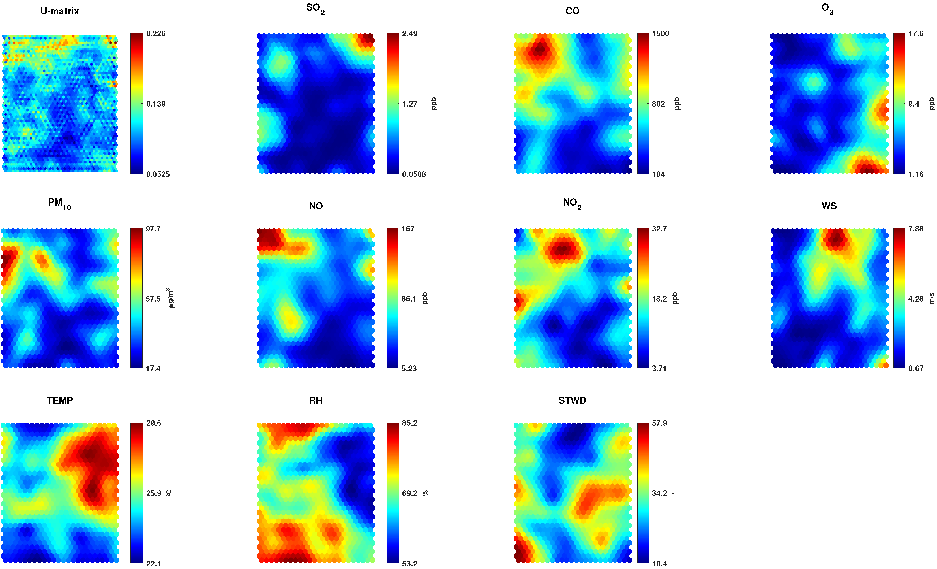
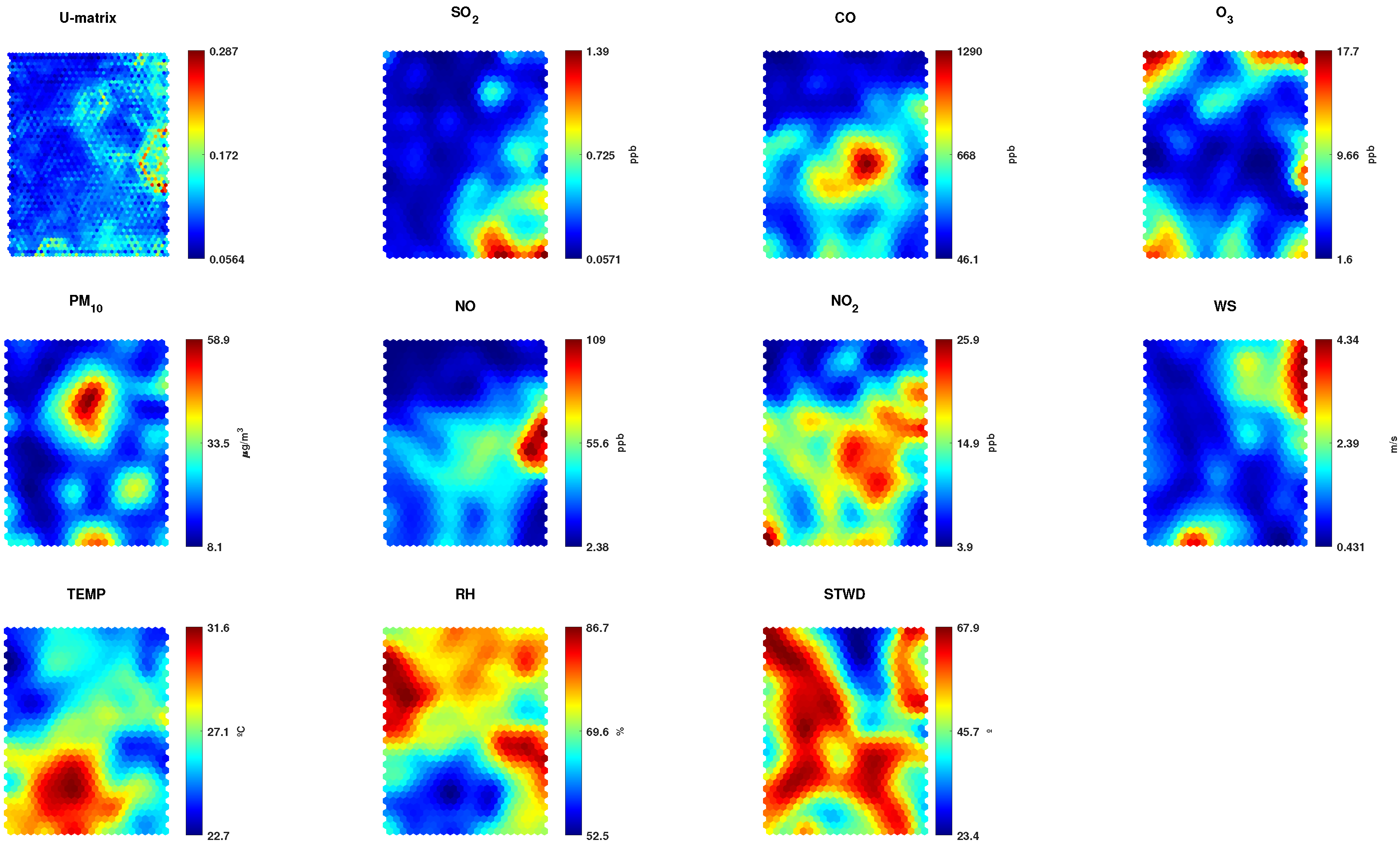
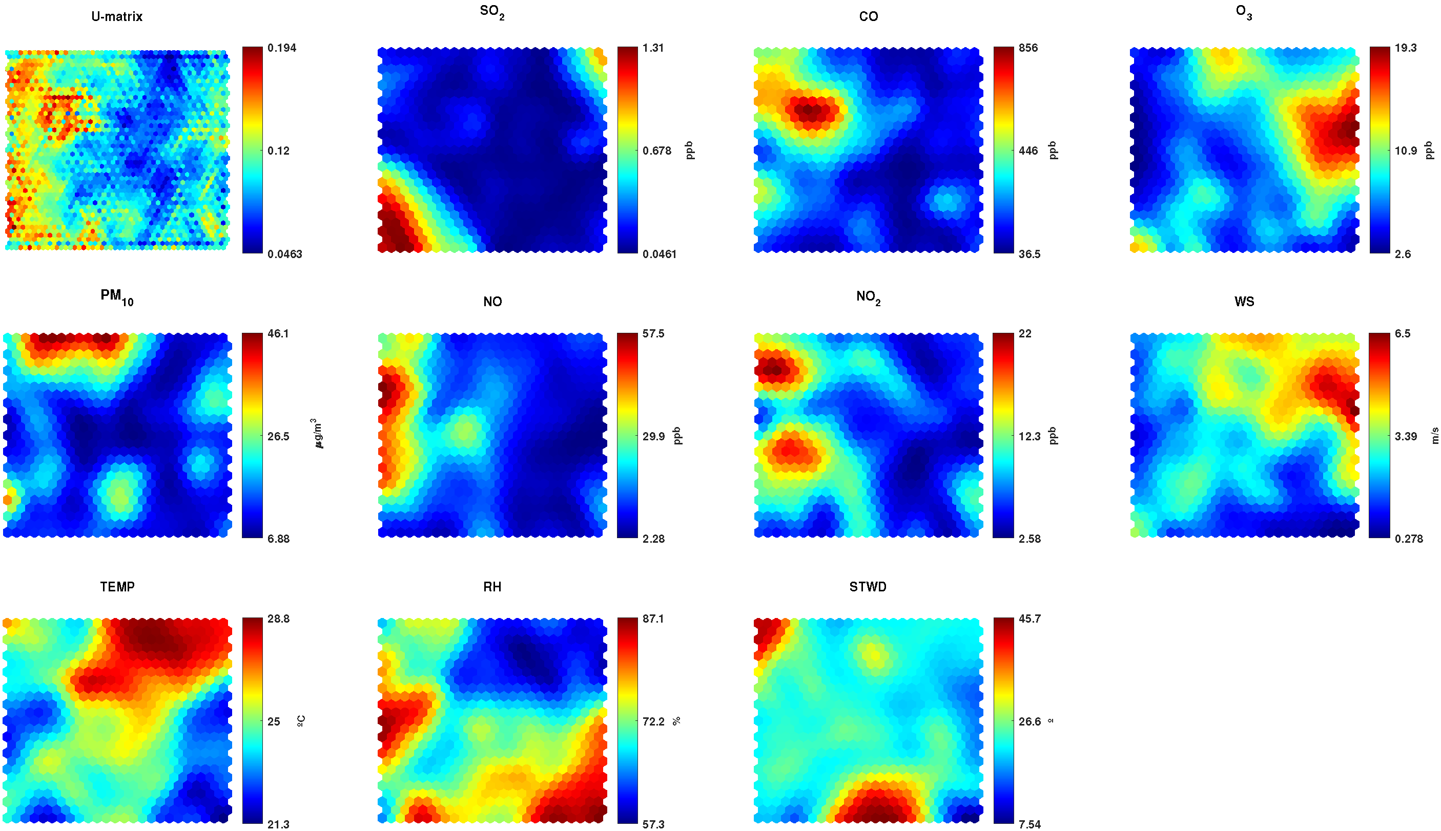
Sustainability 14 10369 g001
Figure 2. Unified distance matrix (U-matrix) and component planes of all analyzed variables (SO2, CO, O3, PM10, NO, NO2, WS, TEMP, RH, and STWD) from the Itaigara station.
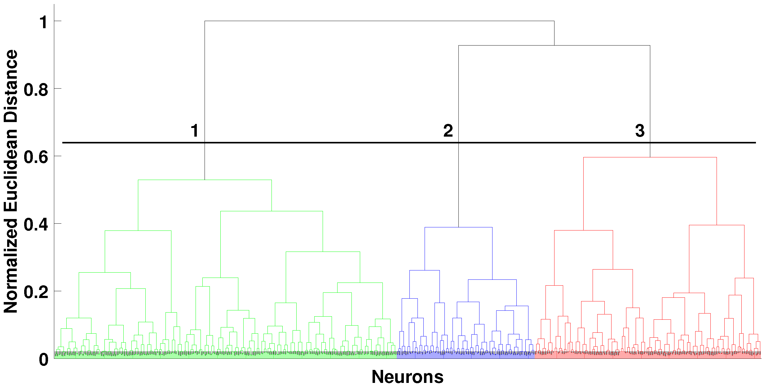
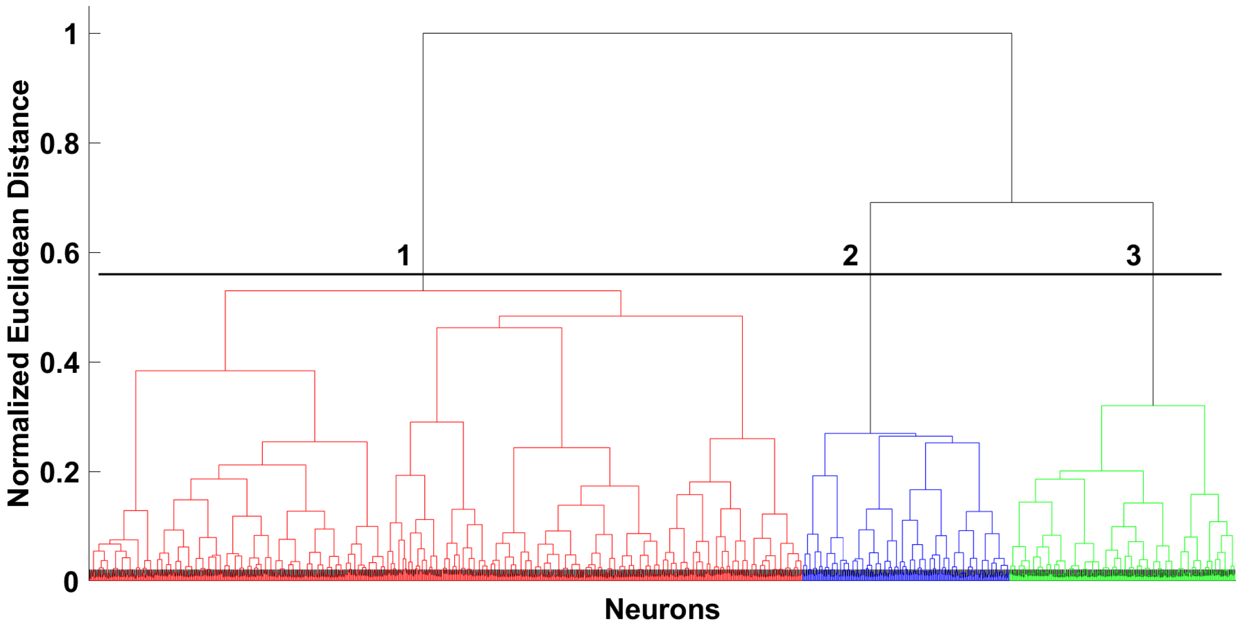
Sustainability 14 10369 g002
Figure 3. Hierarchical analysis of the neurons clusters using the Ward linkage method and Euclidean distance for the Itaigara station.
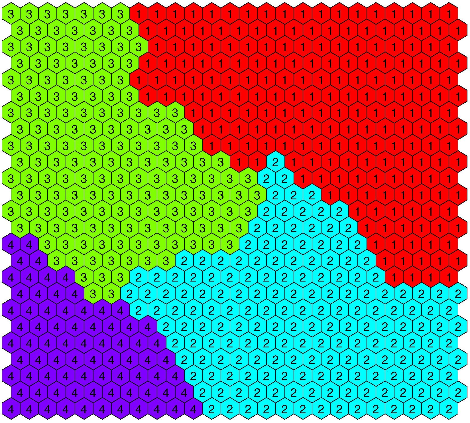
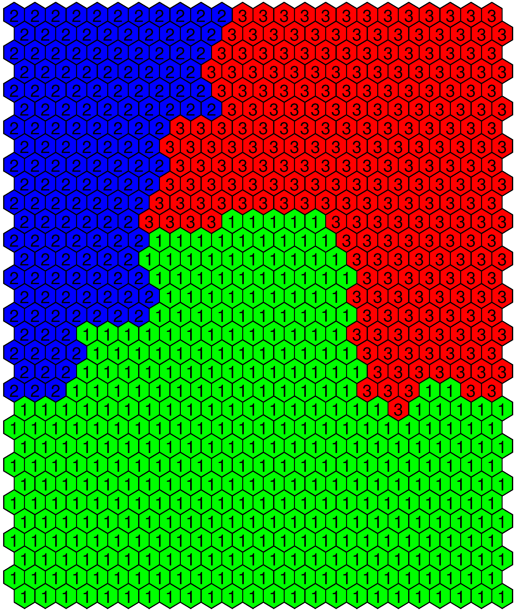
Sustainability 14 10369 g003
Figure 4. SOM neurons grouped into four clusters obtained by the hierarchical analysis of the Itaigara station.
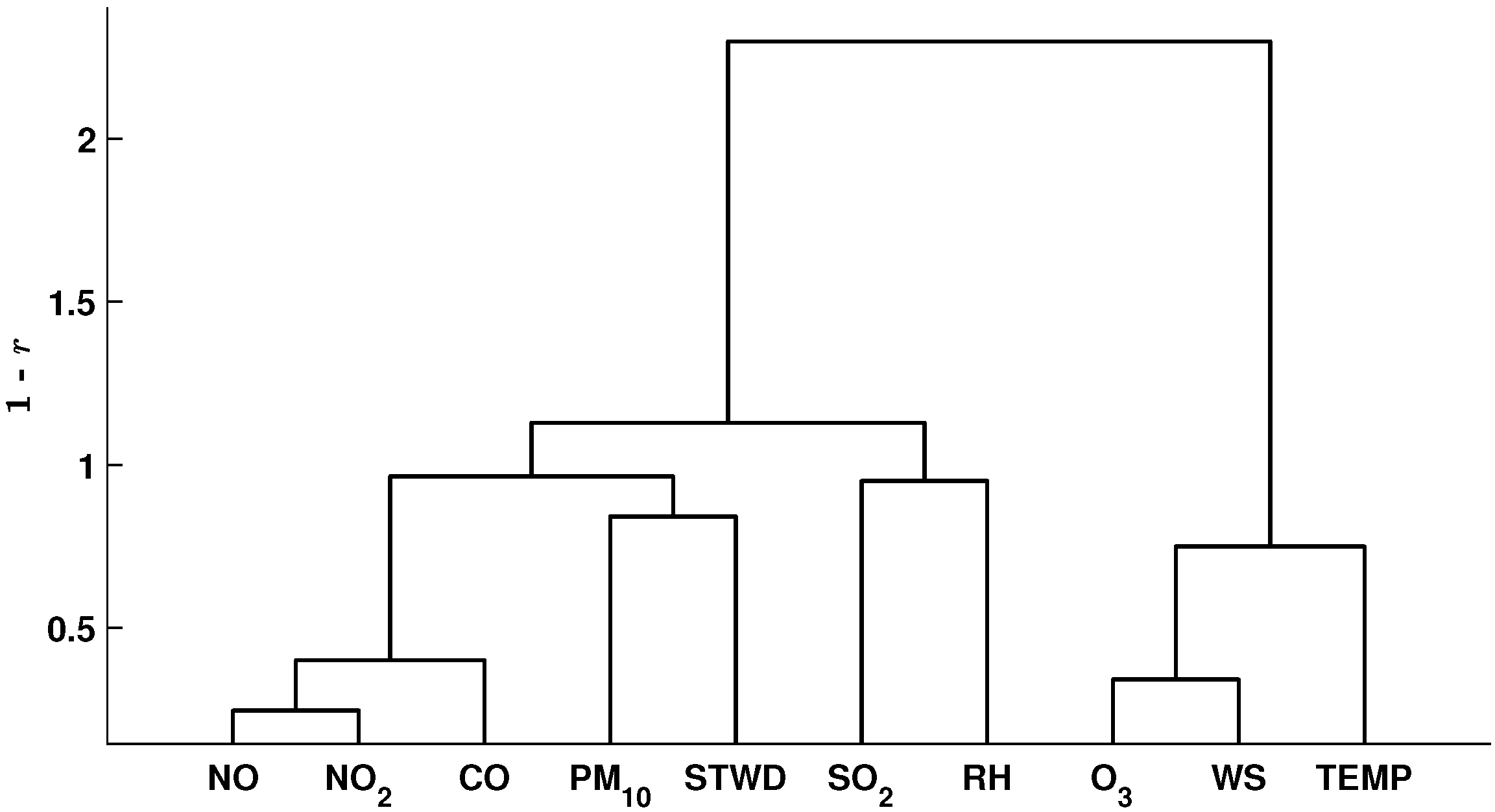
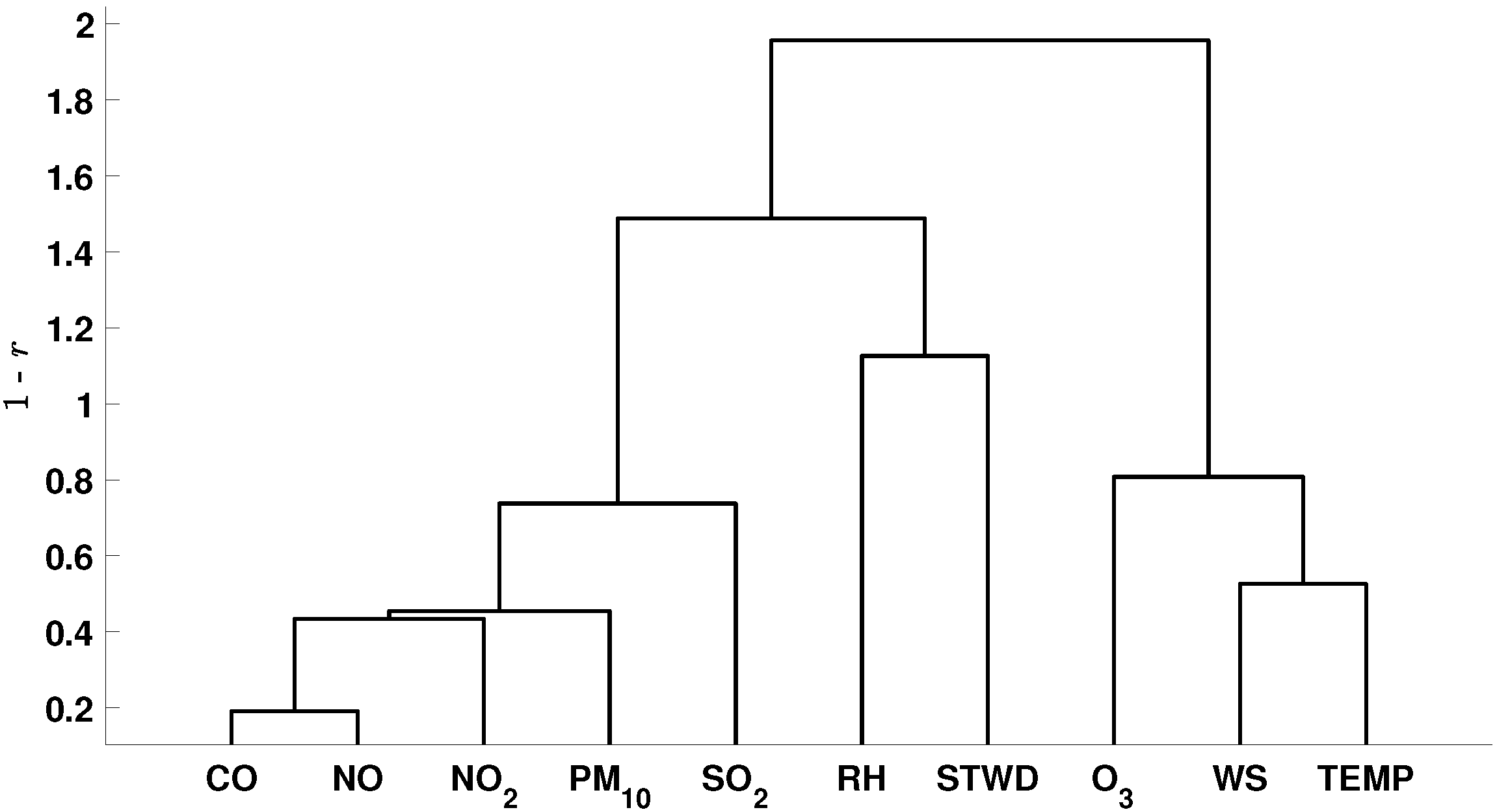
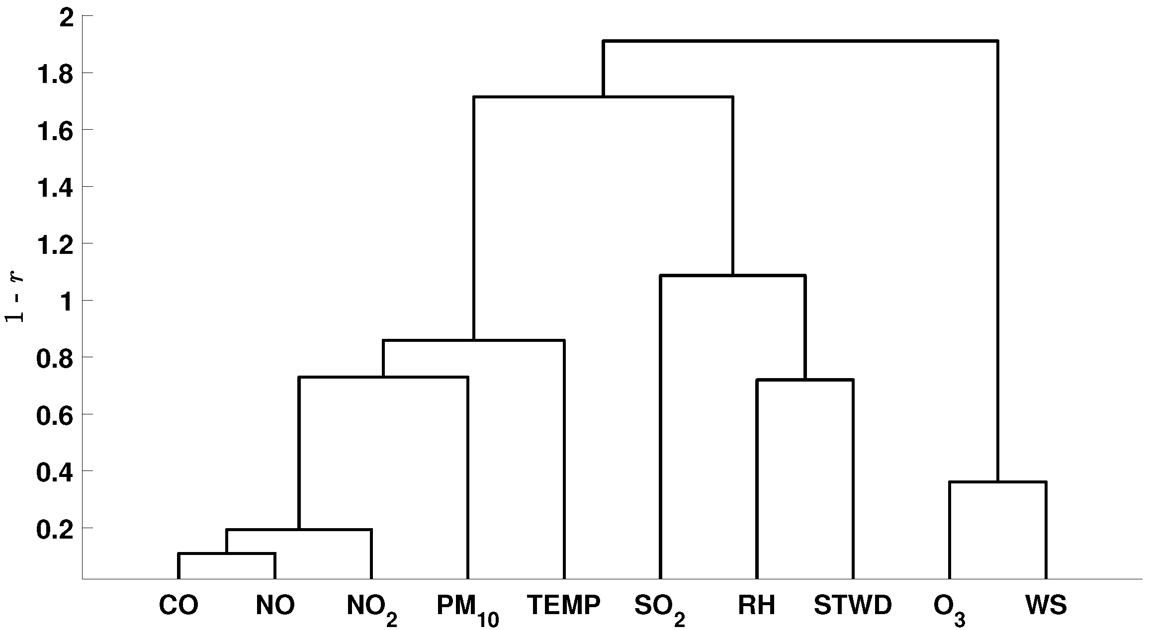
Sustainability 14 10369 g004
Figure 5. Parameter correlation using Ward criterion and distance 1 r , where r is Pearson coefficient, for the Itaigara station.
Sustainability 14 10369 g005
Figure 6. Unified distance matrix (U-matrix) and component planes of all analyzed variables (SO2, CO, O3, PM10, NO, NO2, WS, TEMP, RH and STWD) from the Barros Reis station.
Sustainability 14 10369 g006
Figure 7. Hierarchical analysis of the neurons clusters using the Ward linkage method and Euclidean distance for the Barros Reis station.
Sustainability 14 10369 g007
Figure 8. SOM neurons grouped into three clusters obtained by the hierarchical analysis of the Barros Reis station.
Sustainability 14 10369 g008
Figure 9. Parameter correlation using Ward criterion and distance 1 r , where r is Pearson coefficient, for the Barros Reis station.
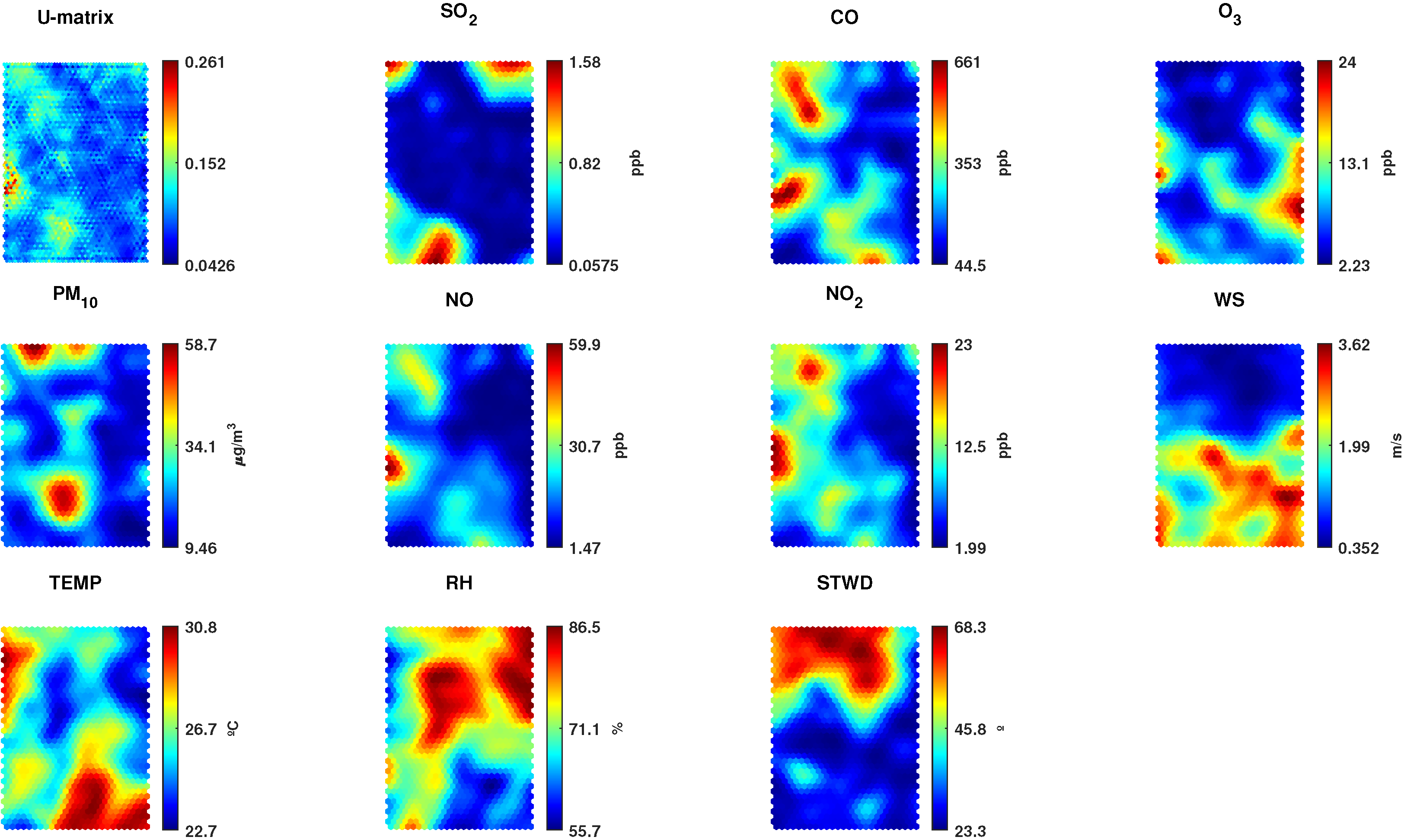
Sustainability 14 10369 g009
Figure 10. Unified distance matrix (U-matrix) and component planes of all analyzed variables (SO2, CO, O3, PM10, NO, NO2, WS, TEMP, RH and STWD) from the Campo Grande station.
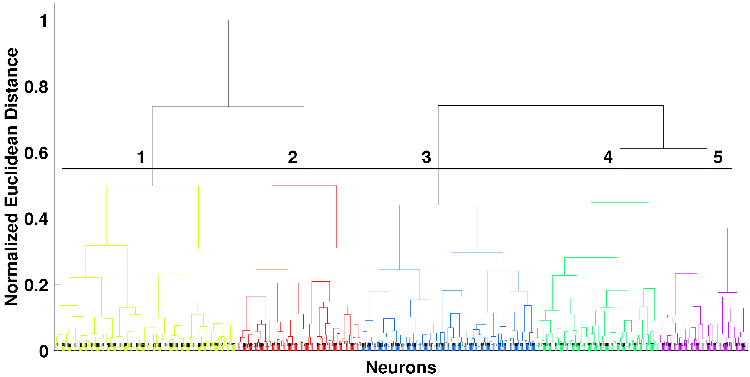
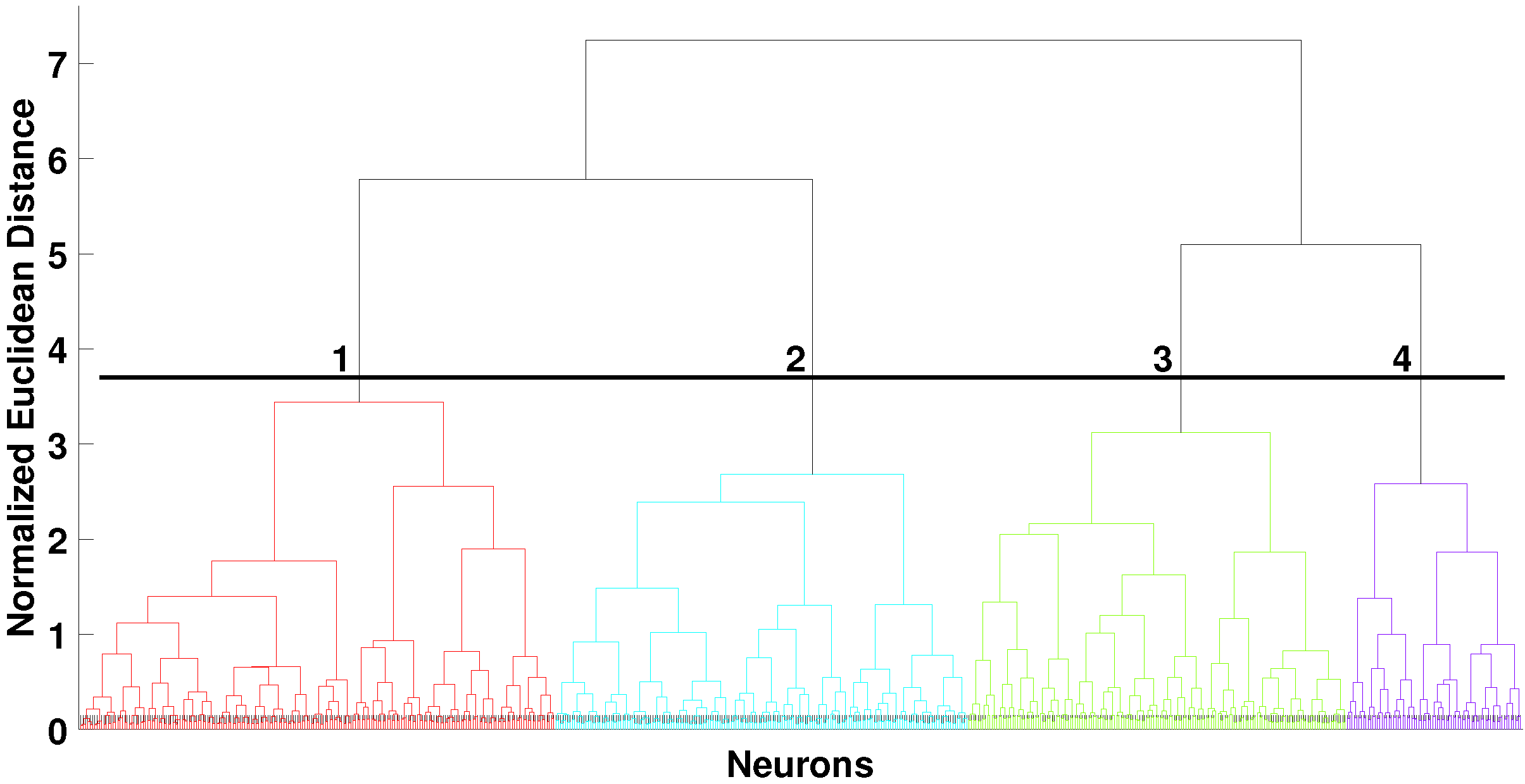
Sustainability 14 10369 g010
Figure 11. Hierarchical analysis of the neurons clusters using the Ward linkage method and Euclidean distance for the Campo Grande station.
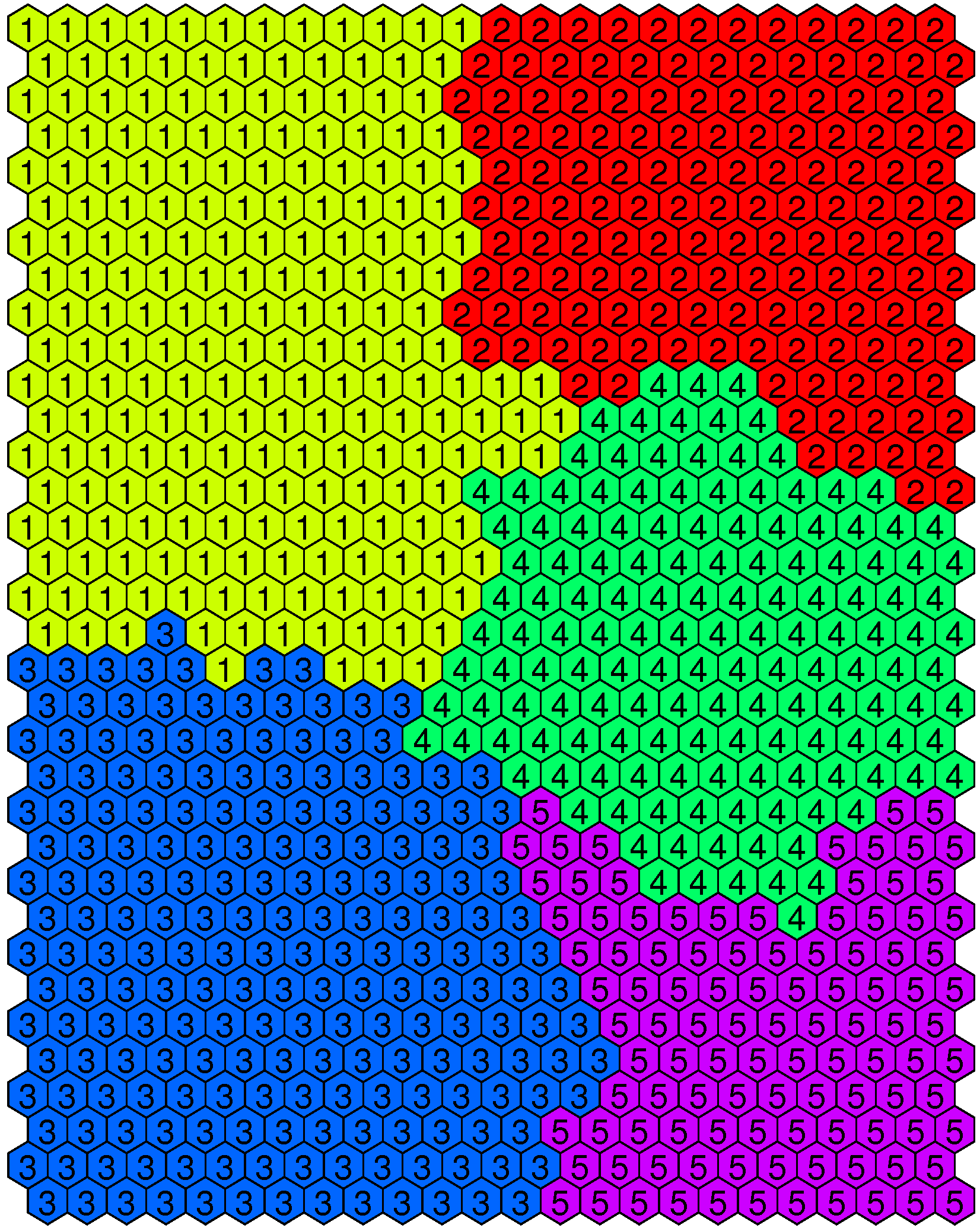
Sustainability 14 10369 g011
Figure 12. SOM neurons grouped into five clusters obtained by the hierarchical analysis of the Campo Grande station.
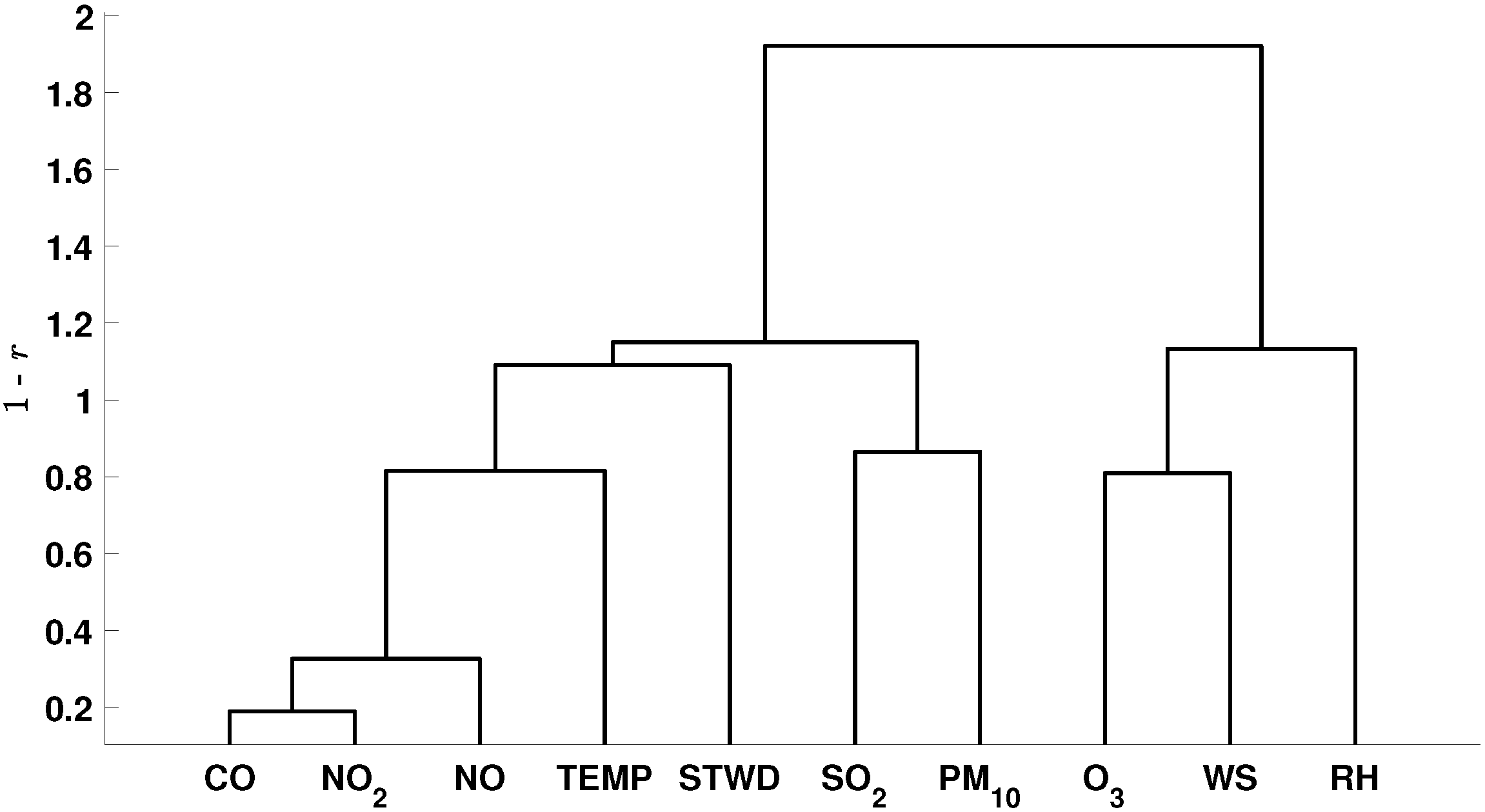
Sustainability 14 10369 g012
Figure 13. Parameter correlation using Ward criterion and distance 1 r , where r is Pearson coefficient, for the Campo Grande station.
Sustainability 14 10369 g013
Figure 14. Unified distance matrix (U-matrix) and component planes of all analyzed variables (SO2, CO, O3, PM10, NO, NO2, WS, TEMP, RH and STWD) from the Dique do Tororó station.
Sustainability 14 10369 g014
Figure 15. Hierarchical analysis of the neurons clusters using the Ward linkage method and Euclidean distance for the Dique do Tororó station.
Sustainability 14 10369 g015
Figure 16. SOM neurons grouped into three clusters obtained by the hierarchical analysis of the Dique do Tororó station.
Sustainability 14 10369 g016
Figure 17. Parameter correlation using Ward criterion and distance 1 r , where r is Pearson coefficient, for the Dique do Tororó station.
Sustainability 14 10369 g017
Table 1. The operation period for each monitoring station provided by CETREL S. A., and the number of data samples available in the dataset before and after the preprocessing step.
StationOperation Start DateOperation End DateNumber of Rregistered SamplesNumber of Samples after Preprocessing
Barros Reis (BR)8 November 201331 December 2016 27 , 584 21 , 559
Campo Grande (CG)2 July 201131 December 2016 48 , 234 24 , 559
Dique do Tororó (DT)19 June 201131 December 2016 48 , 550 42 , 037
Itaigara (IT)18 October 201330 April 2016 22 , 203 15 , 535
Table 2. Descriptive statistics of pollutants and atmospheric data from the Barros Reis station (P = 21,559 samples).
ParametersMagnitureMaximumMeanAverageStandard DeviationVariation Coefficient
SO2ppb3.200.300.450.51112.94%
COppb2180.00570.00601.60335.7055.80%
O3ppb22.704.805.473.8069.36%
PM10 μ g / m 3 129.8037.3040.1019.8849.58%
NOppb206.4044.4052.4738.0172.50%
NO2ppb49.2013.3014.157.6153.84%
WSm/s10.802.202.621.7567.00%
TEMP°C32.5025.5025.632.188.54%
RH%91.0069.0068.609.3113.57%
STWD°73.3031.3031.6111.6136.73%
Table 3. Descriptive statistics of pollutants and atmospheric data from the Campo Grande station (P = 24,559 samples).
ParametersMagnitureMaximumMeanAverageStandard DeviationVariation Coefficient
SO2ppb1.700.200.320.3197.20%
COppb1830.00360.00396.60292.7073.81%
O3ppb25.005.206.014.1869.5%
PM10 μ g / m 3 77.3019.3021.1012.5359.38%
NOppb139.0025.1028.0323.3783.38%
NO2ppb44.0013.3013.376.4248.00%
WSm/s5.101.201.420.9366.01%
TEMP°C34.3026.5026.722.318.66%
RH%94.0072.0071.129.5413.41%
STWD°79.6053.2052.0113.3125.57%
Table 4. Descriptive statistics of pollutants and atmospheric data from the Dique do Tororó station (P = 42,037 samples).
ParametersMagnitureMaximumMeanAverageStandard DeviationVariation Coefficient
SO2ppb2.000.200.330.40123.15%
COppb1000.00220.00239.40163.9068.44%
O3ppb34.307.208.155.3765.88%
PM10 μ g / m 3 75.6020.0022.1312.4256.12%
NOppb73.6012.4013.7711.5483.78%
NO2ppb31.308.208.675.0257.92%
WSm/s6.901.501.631.0161.72%
TEMP°C33.9026.3026.462.318.75%
RH%94.0073.0072.469.1012.56%
STWD°78.8033.0038.4515.3439.90%
Table 5. Descriptive statistics of pollutants and atmospheric data from the Itaigara station (P = 15,535 samples).
ParametersMagnitureMaximumMeanAverageStandard DeviationVariation Coefficient
SO2ppb1.600.100.25020.33131.89%
COppb1210.00190.00226.48207.2691.51%
O3ppb27.507.908.474.3251.00%
PM10 μ g / m 3 67.4013.6016.1610.9867.94%
NOppb70.7011.4015.5013.4586.77%
NO2ppb31.107.308.215.1562.72%
WSm/s10.202.702.761.5857.24%
TEMP°C33.4025.0025.042.279.06%
RH%93.0071.0071.439.0812.71%
STWD°51.3022.8024.328.1333.42%
Table 6. SOM quality measures for Barros Reis Station data (best values in bold).
M h × M v Mz-ScoreMin-MaxLogarithmic
QETEQETEQETE
27 × 24 6481.40320.06490.22900.06360.71730.0606
26 × 26 6761.38980.06870.22730.06610.71080.0616
29 × 24 6961.38870.06680.22700.06680.70960.0607
31 × 23 7131.38050.06310.22590.06070.70510.0593
27 × 27 7291.38030.06120.22450.06530.70320.0629
30 × 25 7501.37660.06600.22500.06670.70170.0616
32 × 24 7681.36840.06490.22320.06220.69770.0601
34 × 23 7821.36520.07010.22290.06440.69500.0644
33 × 24 7921.36090.06550.22240.06730.69570.0587
31 × 26 8061.35970.06580.22190.06630.69480.0622
Table 7. SOM quality measures for Campo Grande Station data (best values in bold).
M h × M v Mz-ScoreMin-MaxLogarithmic
QETEQETEQETE
31 × 23 7131.42160.06660.23840.06260.73460.0625
27 × 27 7291.41870.06600.23820.06670.72940.0584
30 × 25 7501.41310.06500.23690.06640.72770.0626
32 × 24 7681.40820.06480.23600.06400.72530.0630
28 × 28 7841.40990.06190.23520.06850.72300.0610
31 × 26 8061.39940.06450.23410.06700.72150.0589
34 × 24 8161.39480.06420.23400.06240.71930.0592
33 × 25 8251.39490.06360.23340.06360.71730.0593
35 × 24 8401.39250.06510.23360.06690.71630.0630
36 × 24 8641.38980.06190.23240.06430.71460.0594
Table 8. SOM quality measures for Dique do Tororó Station data (best values in bold).
M h × M v Mz-ScoreMin-MaxLogarithmic
QETEQETEQETE
38 × 25 9501.28120.06860.21750.06680.68340.0630
37 × 26 9621.27730.06840.21720.06700.68140.0641
38 × 26 9881.27420.06680.21630.06790.68020.0621
36 × 28 10081.26870.07330.21570.06760.67980.0619
32 × 32 10241.26670.07360.21520.06790.67770.0659
40 × 26 10531.26280.07020.21460.06780.67450.0644
39 × 27 10401.26390.06950.21520.06880.67500.0611
38 × 28 10641.25810.07210.21410.06800.67470.0660
37 × 29 10731.26000.07060.21360.07280.67180.0632
40 × 27 10801.26090.06570.21360.07170.67300.0633
Table 9. SOM quality measures for Itaigara Station data (best values in bold).
M h × M v Mz-ScoreMin-MaxLogarithmic
QETEQETEQETE
24 × 23 5521.43060.05840.24280.05910.77360.0510
26 × 22 5721.42370.06030.24220.05660.77090.0485
24 × 24 5761.42100.06180.24210.05570.77040.0503
27 × 22 5941.41920.05480.24030.05890.76840.0547
25 × 24 6001.41520.05930.24120.05650.76590.0477
27 × 23 6211.41260.05740.24000.05850.76540.0444
25 × 25 6251.40630.05730.23990.05530.76250.0458
27 × 24 6481.40860.05720.23810.05610.75950.0472
26 × 26 6761.39450.06400.23710.05560.75530.0525
27 × 26 7021.38610.05780.23630.05590.75160.0538
Table 10. Parameters’ average values for every cluster formed by the SOM network for the Itaigara station.
ParametersParameter Average Value per Cluster
1234
SO2 (ppb)0.180.090.170.89
CO (ppb)153.18126.03443.43230.86
O3 (ppb)11.937.385.457.61
PM10 ( μ g / m 3 )17.7312.9217.9715.83
NO (ppb)9.209.1529.6419.28
NO2 (ppb)6.106.8112.299.10
WS (m/s)4.151.832.262.20
TEMP (°C)26.4424.1024.8023.97
RH (%)64.3076.9773.1574.38
STWD (°)21.5926.1626.3923.43
#Samples5240446937992027
Table 11. Parameters average values for every cluster formed by the SOM network for the Barros Reis station.
ParametersParameter Average Value per Cluster
123
SO2 (ppb)0.280.640.59
CO (ppb)442.11973.00621.71
O3 (ppb)5.423.037.07
PM10 ( μ g / m 3 )33.3154.0042.13
NO (ppb)37.5491.2251.88
NO2 (ppb)10.7420.2315.68
WS (m/s)1.931.934.12
TEMP (°C)24.6624.7427.68
RH (%)72.6472.1960.05
STWD (°)32.7331.0430.19
#Samples10,59941836777
Table 12. Parameters average values for every cluster formed by the SOM network for the Campo Grande station.
ParametersParameter Average Value per Cluster
12345
SO2 (ppb)0.140.260.230.380.82
CO (ppb)250.98269.62456.78655.67404.37
O3 (ppb)6.127.076.594.155.72
PM10 ( μ g / m 3 )20.0123.7117.6424.4522.21
NO (ppb)15.0718.9730.4756.4924.42
NO2 (ppb)10.3411.1214.3319.1513.12
WS (m/s)0.892.701.401.360.94
TEMP (°C)25.2125.7329.2226.2626.90
RH (%)77.3175.1461.5273.5668.58
STWD (°)57.8242.8353.0550.5052.28
#Samples66404166622342293301
Table 13. Parameters average values for every cluster formed by the SOM network for the Dique do Tororó station.
ParametersParameter Average Value per Cluster
123
SO2 (ppb)0.300.360.34
CO (ppb)245.23342.03130.06
O3 (ppb)9.685.186.05
PM10 ( μ g / m 3 )21.2329.6618.23
NO (ppb)15.1420.063.91
NO2 (ppb)8.7112.135.45
WS (m/s)2.230.670.66
TEMP (°C)26.9027.2224.40
RH (%)69.6571.8881.69
STWD (°)29.1860.4947.53
#Samples26,10175118425
Publisher’s Note: MDPI stays neutral with regard to jurisdictional claims in published maps and institutional affiliations.

