Analysis of the Population Structure and Dynamic of Endemic Salvia ceratophylloides Ard. (Lamiaceae)

Abstract

Understanding how changes of any origin interact with the structure and survival of entire populations is very important for the protection and conservation of threatened, rare and/or endemic species. In this study, structure and population dynamics of Salvia ceratophylloides Ard., a precious endemic species, belonging to the subgenus Sclarea (Moench) Benth., section Plethiosphace Benth. (Lamiaceae) exclusive to the suburban environments of Reggio Calabria (Southern Italy), was analysed. Interactions between this species and its different growth habitats were examined. Moreover, the disturbance factors which directly affect the demographic viability of the species, influencing its growth, reproduction and distribution in its distribution area were identified. From 2019 to 2021, a census by counting individuals of all the known stations, recorded according to a specific protocol, was carried out. The recorded data were statistically analysed and compared with those of the phytosociological surveys carried out using the Braun-Blanquet method and summarised in phytosociological classes, in accordance with the hierarchical floristic classification system of vascular plant communities, accepted at national and European levels. The structure of the different populations was also related to the different threat factors that afflict S. ceratophylloides. It was observed that the most structured populations of S. ceratophylloides were found in natural and semi-natural environments where the anthropogenic disturbance was minor, while populations with an irregular structure were found in sites exposed to disturbances of various origins. The different phytosociological classes do not interact directly on population structure. The most important factors affecting structure and distribution are disturbances of various origins, in particular anthropogenic and phytosanitary disturbances. In order to keep populations balanced and stable over time, it would be useful to adopt conservation measures for the species and the habitat in which they live, with practical solutions for the following: (a) to limit infestations by insects that parasitize stems and seeds; (b) to prevent mowing, fires, grazing and the introduction of invasive alien species.

1. Introduction

A useful tool for the conservation and management of rare and threatened plant species is knowledge of the relationships between population dynamics, vegetation and habitat [1]. Managing the conservation of these populations requires a detailed understanding of the life cycle of the species under study and the temporal variations of “life stages” [2,3].

Critical phases in the life cycle of rare plants can be detected through the study of population dynamics [4,5,6]. These studies can highlight what factors interfere with, and influence, population trends, and whether these are related to threats to the species, the structure and composition of the surrounding vegetation or different management, control and land-use practices [7]. Through this analysis, it is possible to use a forecasting approach as to what the effects of ecological changes on threatened populations might be [1,8,9]. However, the laboriousness and the timelines associated with this type of study prevent their widespread use in conservation biology [10].

A faster method of conducting population analyses of perennial (herbaceous) plants is to analyse their structure in a single census. The structure of a population can be described by classifying individual plants by age and size, or by considering the different phenological stages of the individuals that compose a population, generally referred to as “life stages” [6,11].

Population dynamics are also strongly influenced by climate change, which, in recent years, is having very serious impacts on flora and fauna [12,13,14,15,16]. As a consequence of climate change, a distributional shift of plant species to higher altitudes and latitudes is expected. This will be almost impossible for rare and/or endemic taxa, which are tightly bound to a narrow ecological niche and exclusive to a specific range, which is very often fragmented [14,17,18,19,20]. In addition, a further threat is posed by alien species, which, finding favourable temperatures, rapidly expand their range, competing with native species and causing the loss of habitats that preserve rare and/or endemic species [21,22,23,24].

The Lamiaceae family is one of the biggest group of plants which have several properties due to their rich composition in essential oils, and are considered, for this reason, an important group of Medicinal Aromatic Plants (MAPs) [25,26]. They are also valued as ornamental plants, and as culinary and medicinal herbs, making them a group of exceptional ecological, ethnobotanical and floristic importance [27]. The genus Salvia, spread from the Far East through Europe to the New World, represents a cosmopolitan group with nearly 1.000 species, resulting in one of the largest genera belonging to this family [28]. It is present in the pharmacopoeia of many countries around the world, where it assumes a very important economic role; numerous species are used for medicinal, food, and ornamental purposes [29,30]. The genus Salvia has a very wide range, occurring in Central and South America with 500 spp., 250 spp. in Central Asia/Mediterranean and 90 spp. in East Asia [28]. According to European flora [31], the genus Salvia occurs in Europe with 36 species, 3 subspecies, 3 hybrids and 2 aliens. In a more recent work, Nikolova & Aneva [32], counted 39 species and 1 subspecies for Europe.

The Italian flora, to date, includes 28 species and 6 subspecies of the genus Salvia, of which 11 taxa allochthonous, and 22 native, of which 4 are endemic [33], these include Salvia ceratophylloides Ard., a rare endemism exclusive to the suburbs of Reggio Calabria (Southern Italy) (Figure 1). Hedge [31] and Nikolova & Aneva [32] do not recognize S. ceratophylloides as a separate species, considering it a synonym of S. pratensis. On the contrary, Pignatti [34,35] recognizes it as an endemic species, exclusive to southern Calabria.

Salvia ceratophylloides belongs to the subgenus Sclarea (Moench) Benth., section Plethiosphace Benth., characterised by a campanulate calyx, above two grooves, concave, with three conniving teeth and corolla with a crescent-shaped, compressed upper lip [36]. It is part of the S. pratensis group present in Italy with some entities: S. pratensis L. subsp. pratensis, S. pratensis L. subsp. saccardina (Pamp.) Poldini, S. haematodes L., S. virgata Jacq. and S. ceratophylloides Ard. [35]. Del Carratore and Garbari [36], in their study on the section Plethiosphace, report the following for Italy: Salvia clandestina L., S. haematodes L., S. pratensis L., S. saccardiana (Pamp.) Del Carr. and Garbari, S. verbenaca L., S. virgata Jacq., and considered S. ceratophylloides extinct, as it has not been found in recent decades.

Already in 1800 [37,38] this species was known in the Reggio Calabria area in several localities. Subsequent reports date back to the first two decades of the 20th century [39], when the species was considered extremely rare [40]. The profound environmental transformations undergone by the suburban area of Reggio Calabria, due to intense urbanisation and the devastating fires that ravage the territory, has brought about profound changes in the landscape with the reduction, degradation and disappearance of natural habitats. As a result, in the localities mentioned in the letter (Gallico Superiore, Terreti, Straorino, Ortì, Vito Superiore, Pietrastorta) [40] S. ceratophylloides was no longer found, despite searches by various botanists. So, in 1997, it was declared extinct and listed in the ‘Red Book of the Flora of Italy’ as ‘Extinct in the Wild’ (EW) [41]. Its extinction was confirmed by later authors who studied the genus Salvia in Italy [42] and by Scoppola and Spampinato [43] in the “Atlas of Endangered Species” of the Italian flora. Field research, however, made it possible to find four micro-populations of the species at different locations (Puzzi and Cataforio) in 2008. The populations consisted of a few dozen breeding individuals and were about 10 km away from the populations previously reported in the literature [44]. Subsequent studies over time have made it possible to verify the presence of the species in other localities and to define its conservation status and taxonomic and ecological characteristics in relation to related species [19].

The objective of this study was a careful census of the existing population in order to define the actual distribution and composition and the correlations between population distribution, vegetation and threats to the species’ habitats. Understanding the interactions between populations and habitats, and how these may affect population dynamics and survival over time, is of fundamental importance in understanding the strategy to safeguard endangered taxa, especially when they are endemic.

2. Materials and Methods

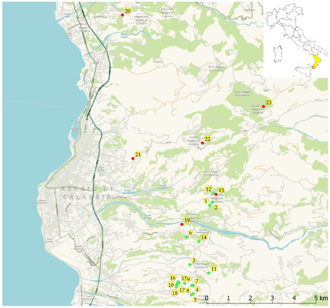
2.1. Study Area

The distribution area of S. ceratophylloides falls in southern Italy (South Calabria) and is entirely within the municipality of Reggio Calabria. Field research carried out between 2017 and 2021, ascertained the presence of the species in various localities (Puzzi fraz. di Gallina (Serro dei Morti and Serro d’Angelo), Mosorrofa (Serro Ciugna) and Mosorrofa Vecchio, Aretina (Serro della Cattina, Prai), San Todaro, Armo (Spilingari and Grotta di Sant’Arsenio). A total of 17 micro-populations are known to date, all distributed in the suburban periphery of Reggio Calabria (Figure 2).

Table 1. Climatic parameters referred to Armo locality (Reggio Calabria) (these data were obtained from the NASA Langley Research Center (LaRC) POWER Project funded through the NASA Earth Science/Applied Science Program [45]).

Parameter	1991/2021	2019	2020	2021
Specific Humidity at 2 Meters (g/kg)	9.59	9.7	9.58	9.64
Relative Humidity at 2 Meters (%)	71.52	70.88	69.56	70.06
Temperature at 2 Meters Maximum	35.43	35.19	34.13	38.08
Temperature at 2 Meters Minimum	4.64	4.43	6.55	4.44
Temperature at 2 Meters Range	30.79	30.76	27.59	33.64
Precipitation Corrected (mm/day)	1.86	1.85	1.54	1.94
Precipitation Corrected Sum (mm)	609.68	606.45	511.52	706.65

shows the climatic parameters of humidity, temperature and precipitation in the time range 1991–2021 and in the years 2019, 2020, 2021.

These climatic parameters do not affect the population trend of S. ceratophylloides and they did not change significantly over the 3 years of the survey; in fact, they remained within the average calculated over the 30-year period 1991–2021.

The bioclimate of this area is typically Mediterranean Pluviseasonal [46] with average annual temperatures of 18 °C and average annual precipitations of about 600 mm, centralised in the autumn months of November and December. It is characterised by a summer dry period of about 5 months [19].

Salvia ceratophylloides grows at altitudes between 260 and 380 m a.s.l., on sandy substrates alternating with soft limestone beds of Pleistocene and Pliocene origin [47].

2.2. Population Analysis

The population census was carried out for three consecutive years (2019–2020–2021), in June, using the protocol proposed by Hegland et al. [11], in a study on the population dynamics of Salvia pratensis, a species related to S. ceratophylloides in terms of biological and phenological characteristics. The census covered the entire current population of this endemic point species.

In order to facilitate the population census, the micro-populations of the species were subdivided into sub-areas with similar habitats, on which the count of individuals was carried out distinguishing the different “life stages” (Table S1). Micro-population 13, which had only one plant in 2018 [48], was omitted from the census because it became extinct in the following years.

In each sub-area, individuals were surveyed, distinguishing five “life stages” (Figure 3):

S = Seedlings, with cotyledons and one/two main leaves.

JI = (J) Juveniles with two/three pairs of leaves and (I) Immature plants with three/four pairs of leaves. In Hegland et al. [11] these two “life stages” are considered distinct: in this work it was preferred to unify the data, since for S. ceratophylloides it is impossible to distinguish the two phenological stages as described for S. pratensis.

V = Vegetative adults with at least five pairs of leaves.

G = Generative adults having one to five flowering stems up to 50 cm high. Within the G category, two size sub-classes have been distinguished: SG = Small Generative adults with one or two flowering stems; LG = Large Generative adults with more than two flowering stems, usually the largest individuals are also the oldest (3–4 years old).

In each sub-area, the population density and the increase and decrease over the 3 years of the survey were estimated using the Malthusian exponential growth model [49].

$$N_t=N_0{e}^{rt}$$

where:

• $N_0$ is the number of individuals at time zero (No. of individuals in 2019);
• $N_t$ is the number of individuals after a certain time interval (No. Individuals in 2021);
• $e$ is the Euler number;
• $r$ is the intrinsic population growth rate for each individual and for each unit of time considered (the difference between births and deaths in the unit of time);
• $t$ is the time from $t_0$ to the year considered.

In particular:

$$r=\ln \left(R\right)$$

$R$ is the net fundamental growth rate per capita, and indicates the average contribution of each initial individual to the population after the time interval has elapsed. It integrates both the survival of individuals and the birth rate, referred to the time interval.

$$R=N_0/N_t$$

In order to assess future population trends, assuming constant ecological and environmental conditions, the variations (increase or decrease) of the different population types revealed by cluster analysis were estimated over a five-year period.

2.3. Habitat Characterisation and Georeferencing

In order to characterise the habitat of S. ceratophylloides in each micro-population, ecologically and physiognomically homogenous sub-areas were identified, on which vegetation analysis was carried out using the phytosociological method [50,51,52].

Taxa nomenclature is according to Bartolucci et al. [53] and the relevant updates in the Portale della Flora d’Italia [33].

For each species, the relevant phytosociological class was considered in accordance with Mucina [54] and the Prodromo alla Vegetazione d’Italia [55].

All micro-populations of S. ceratophylloides were uniquely recorded, georeferenced and entered into a shapefile processed with QGIS 2.18.7^® (OSGeo, Beaverton, OR, USA) (Figure 2).

2.4. Pressures and Threats

For each sub-area, the pressures and threats acting on the habitat were analysed and coded according to the “Reference list Threats, Pressures and Activities” by Salafsky et al. [56], modified by the European Environment Information and Observation Network (EIONET) [57]. The different threats were estimated in relation to their importance: low (L), medium (M) or high (H). In order to quantify the pressures, the importance values were expressed numerically (1 = low L; 2 = medium M, 3 = high H) (Table S3).

2.5. Statistical Analysis

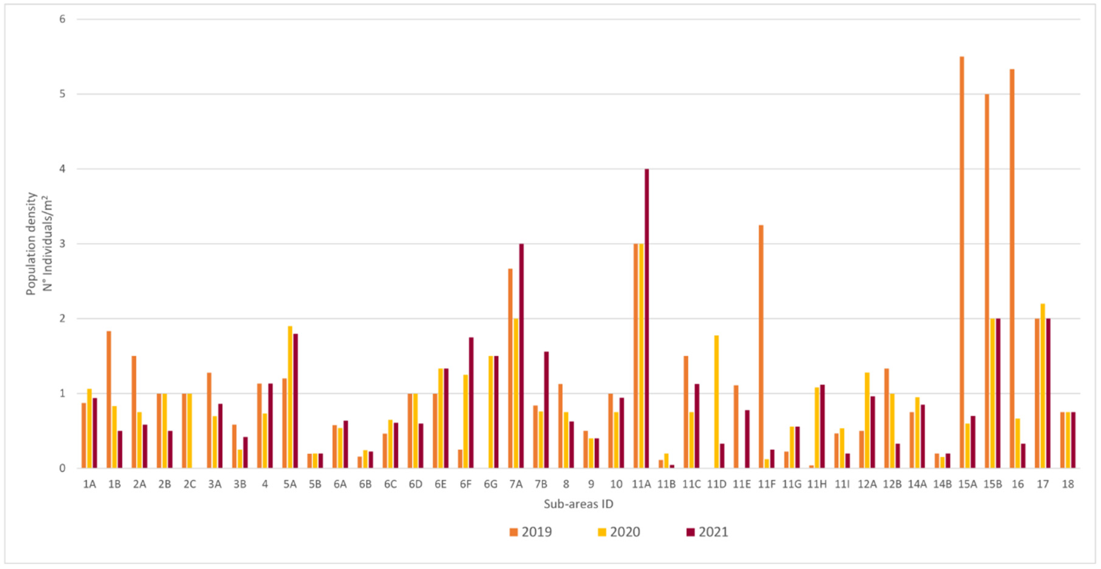
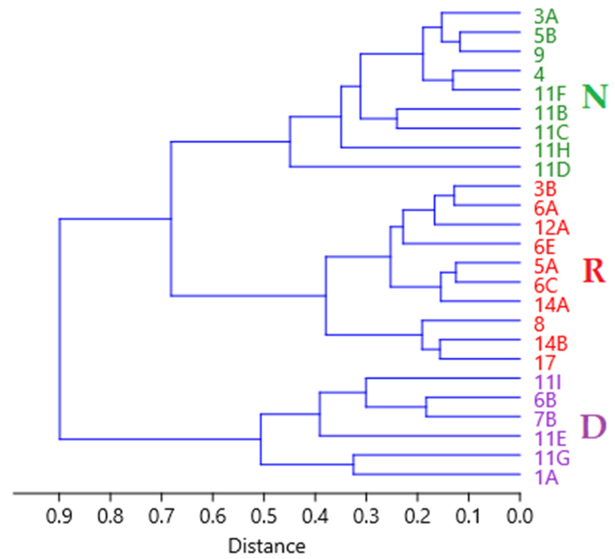
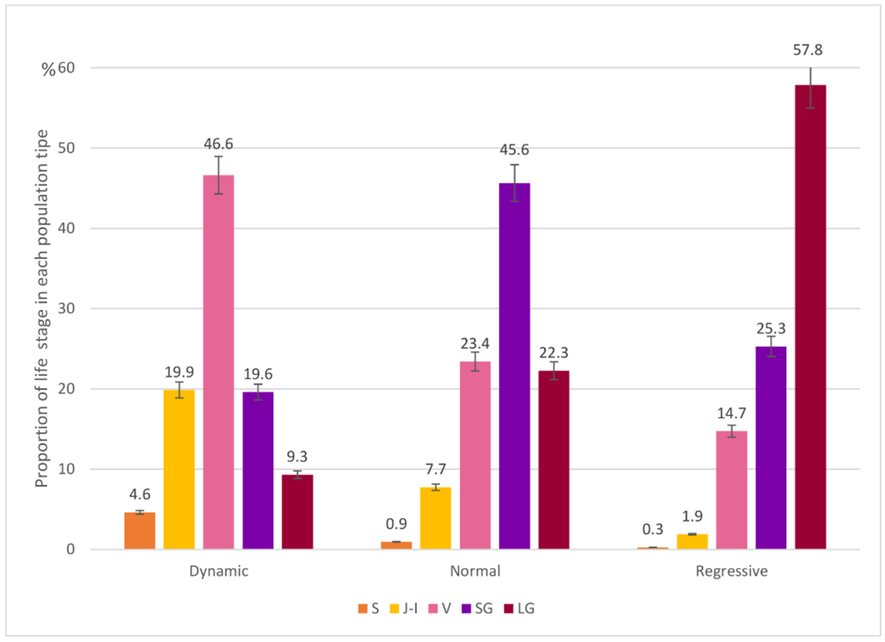
Data on population structure, threats and vegetation were entered into matrices using Microsoft Excel© 2019 (Microsoft Corporation, Redmond, WA, USA). For statistical analyses, three-year averages of the data were calculated and transformed into percentages. The life stage data of each sub-area were used to analyse the degree of similarity by means of hierarchical cluster analysis with the group average method (UPGMA), chord distance for ratio scale data, and K-means clustering [58]. The Past 4.10© software (Hammer, Oslo, Norway) [59] was used for both statistical analyses. The population groups that the cluster highlighted in relation to the “life stage” ratios, in accordance with Hegland et al. [11] and Oostermeijer et al. [60], can be defined as “Dynamic”, characterised by high ratio [(S + JI + V)/G] between breeding and non-breeding individuals, “Normal”, with a balanced ratio between breeding and non-breeding and “Regressive”, with a low ratio between breeding/non breeding. Sub-areas with a very small number of individuals (>10) occupying areas of less than 10 m² were excluded from the statistical analysis as they were not significant.

To measure the strength of the relationships between the different “life stages” in relation to pressures and vegetation, the correlation coefficient was calculated using Microsoft Excel© 2019 software: this value is between +1 and −1, indicating a positive (+1) or negative (−1) correlation between the matrices. In the linear regression, the different “life stages” were used as dependent variables and the different pressures as independent variables.

The equation for calculating the correlation coefficient is:

$$Correl \left(X,Y\right)=\frac{\sum \left(x-\overline{x}\right)\left(y-\overline{y}\right)}{\sqrt{\sum {\left(x-\overline{x}\right)}^{2 }}\sum {\left(y-\overline{y}\right)}^2}$$

where: $\overline{x}$, $\overline{y}$ are the mean values of the first matrix (“life stage”) and mean values of the second matrix (threats; vegetation) of the sample mean.

For the correlation value, the linear regression test was carried out for all parameters considered previously, using the least squares method; this processing was also carried out using Microsoft Excel© 2019 software.

The equation defining the linear correlation is as below:

$$Y_i={\beta }_0+{\beta }_i{X}_i+\epsilon$$

where:$i$ is the number of observations,$Y_i$ is the dependent variable (which in our case coincides with the different “life stages”), $X_i$ is the independent variable (which coincides with threats or vegetation),

$${\beta }_0+{\beta }_i{X}_i$$

is the regression function where: ${\beta }_0$ is the intercept of the regression line (it represents the value of $Y$ when $X$ is equal to 0), ${\beta }_i$ represents the gradient of the line (it is the angular coefficient of the regression line i.e., the rate of change of $Y$ when $X$ changes). $\epsilon$ is the stochastic error and represents the difference between the actual value of a dependent variable and its predicted value.

The residuals obtained from the linear regression analysis were analysed graphically by constructing Q-Q plots (quantile-quantile graphs), which made it possible to verify their normally distributed trend in order to obtain confirmation of the validity of the linear regression model.

Co-occurring data on plant species cover (excluding S. ceratophylloides and those species found to be less frequent in the surveys) were analysed by Detrended Correspondence Analysis (DCA) [61] using R© software (Foundation for Statistical Computing, Vienna, Austria).

3. Results

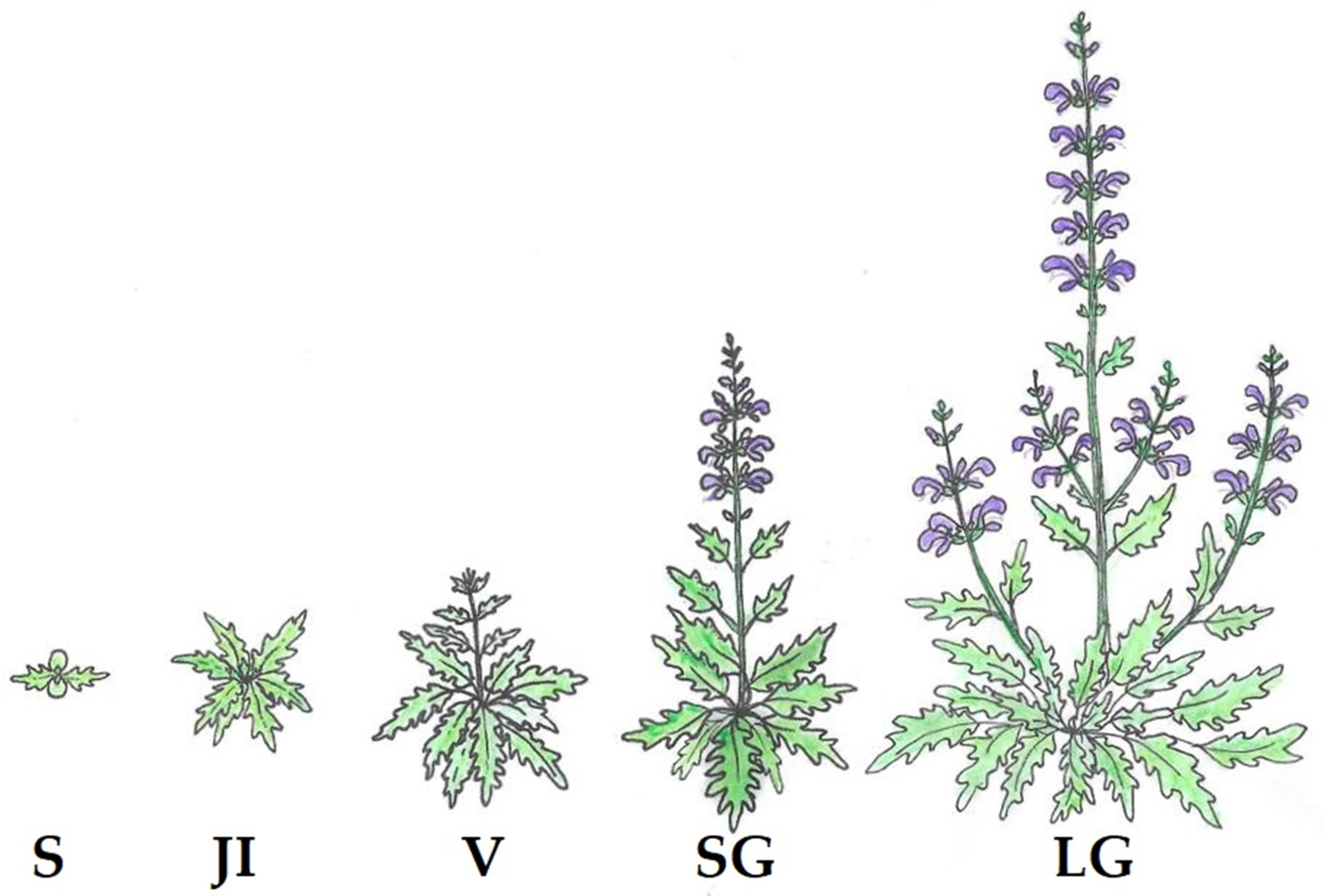
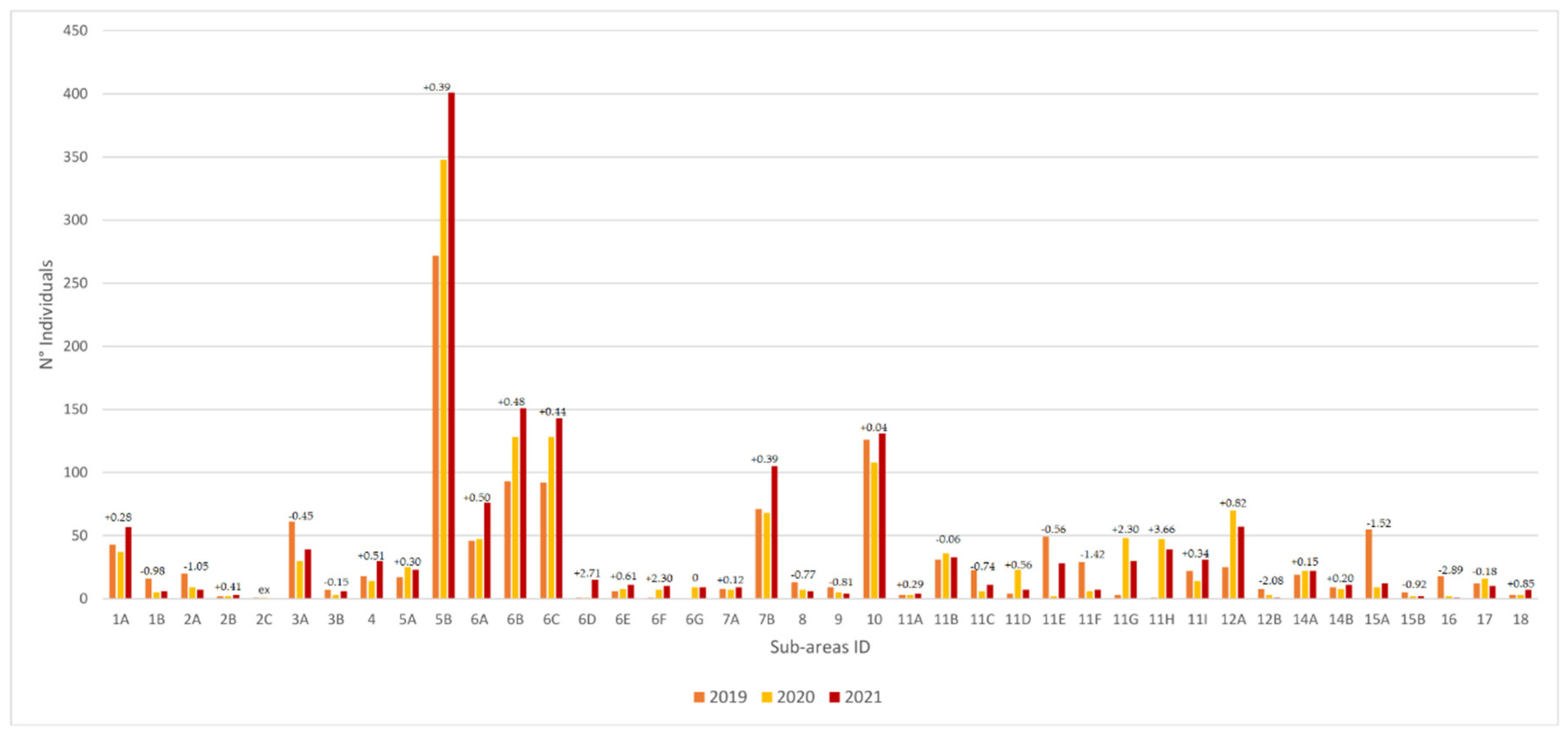
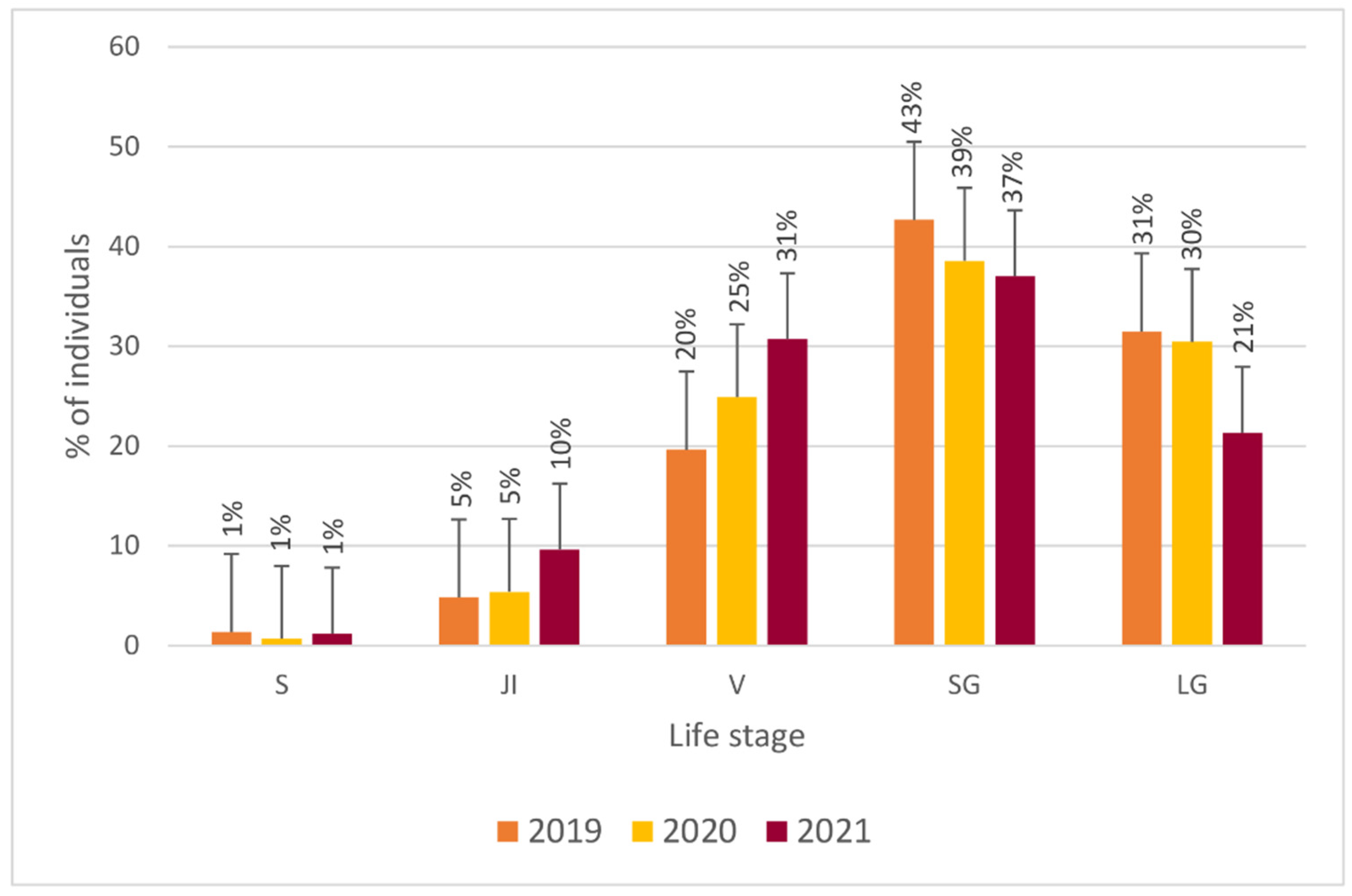
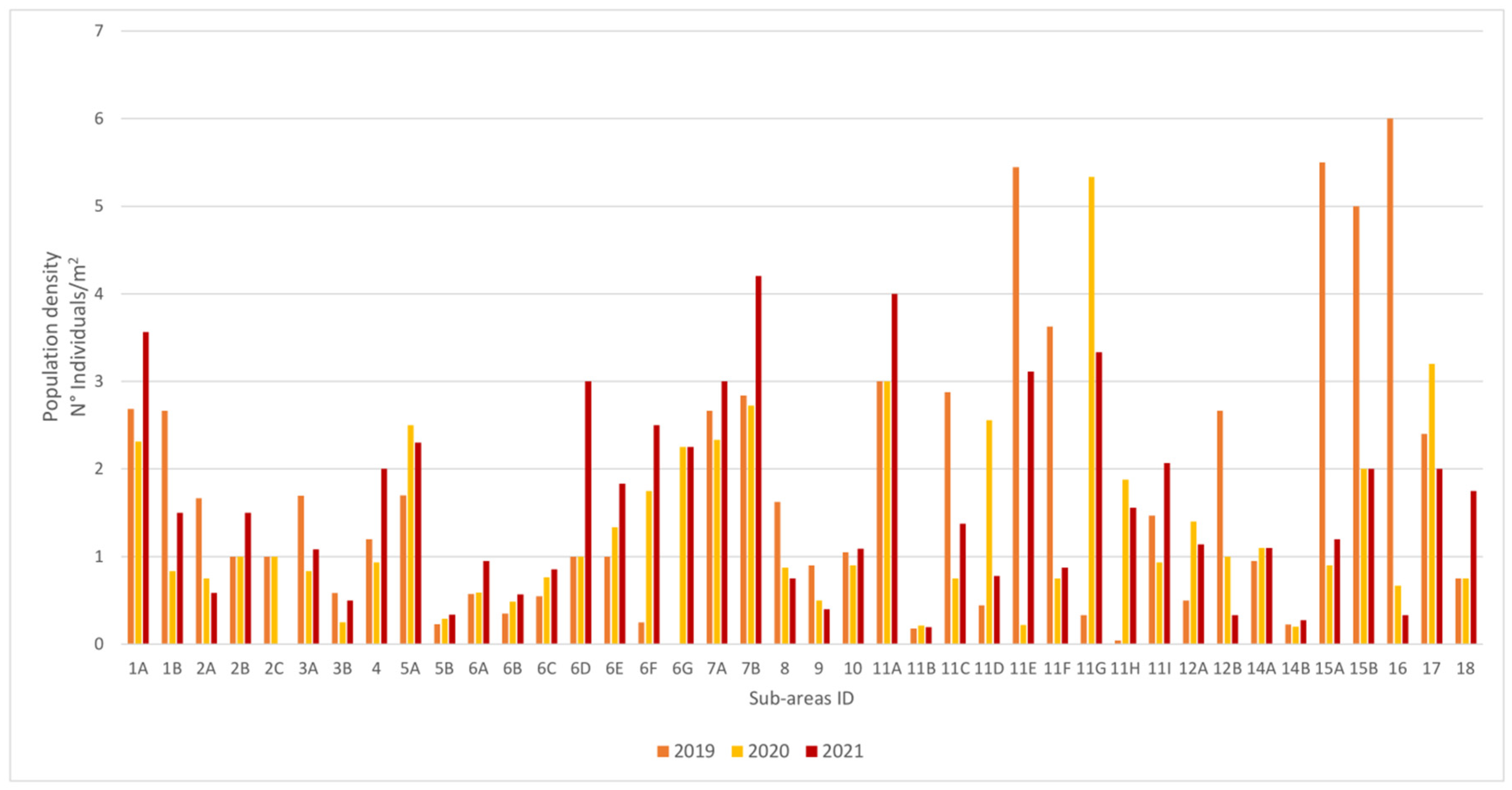
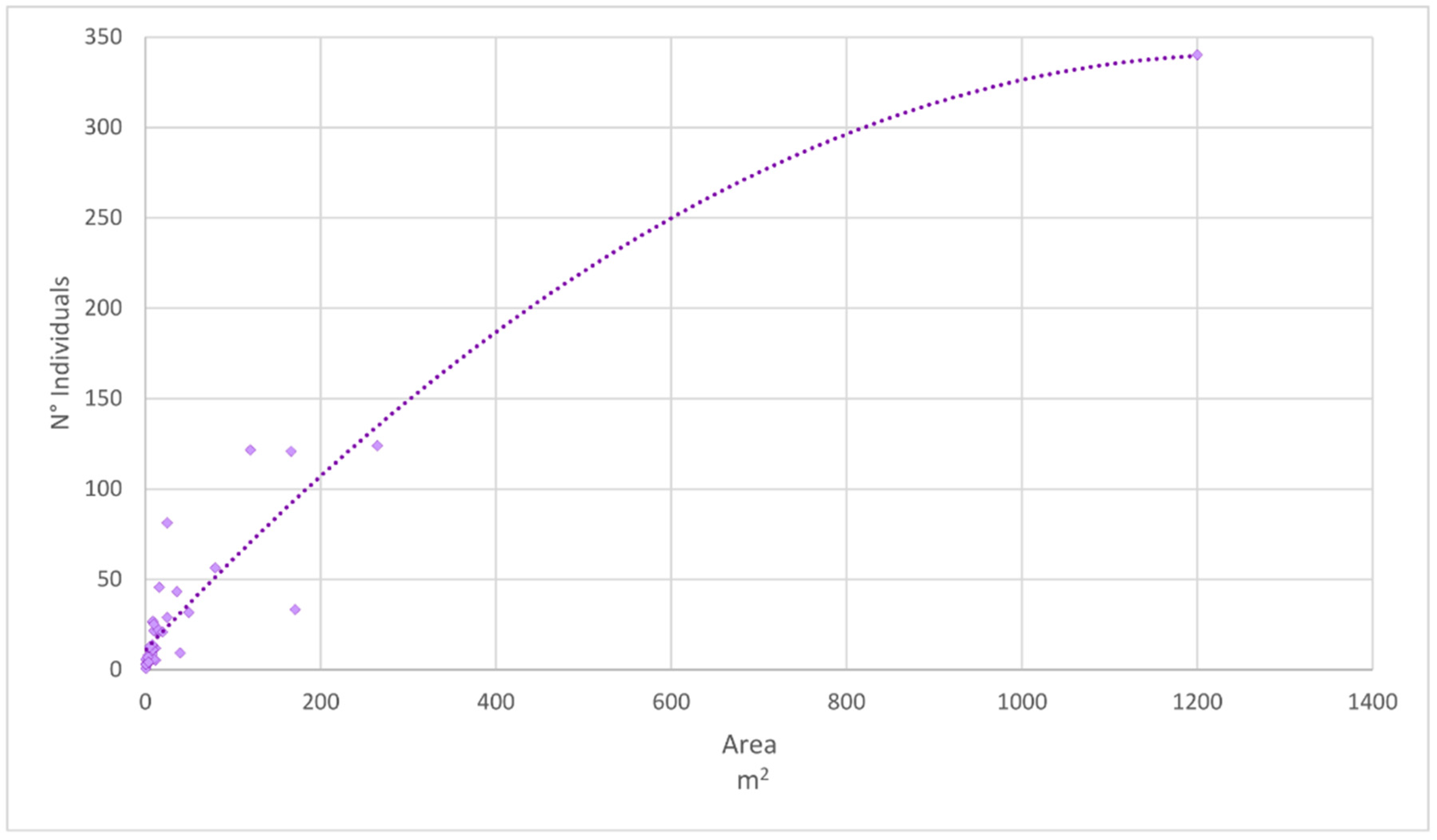
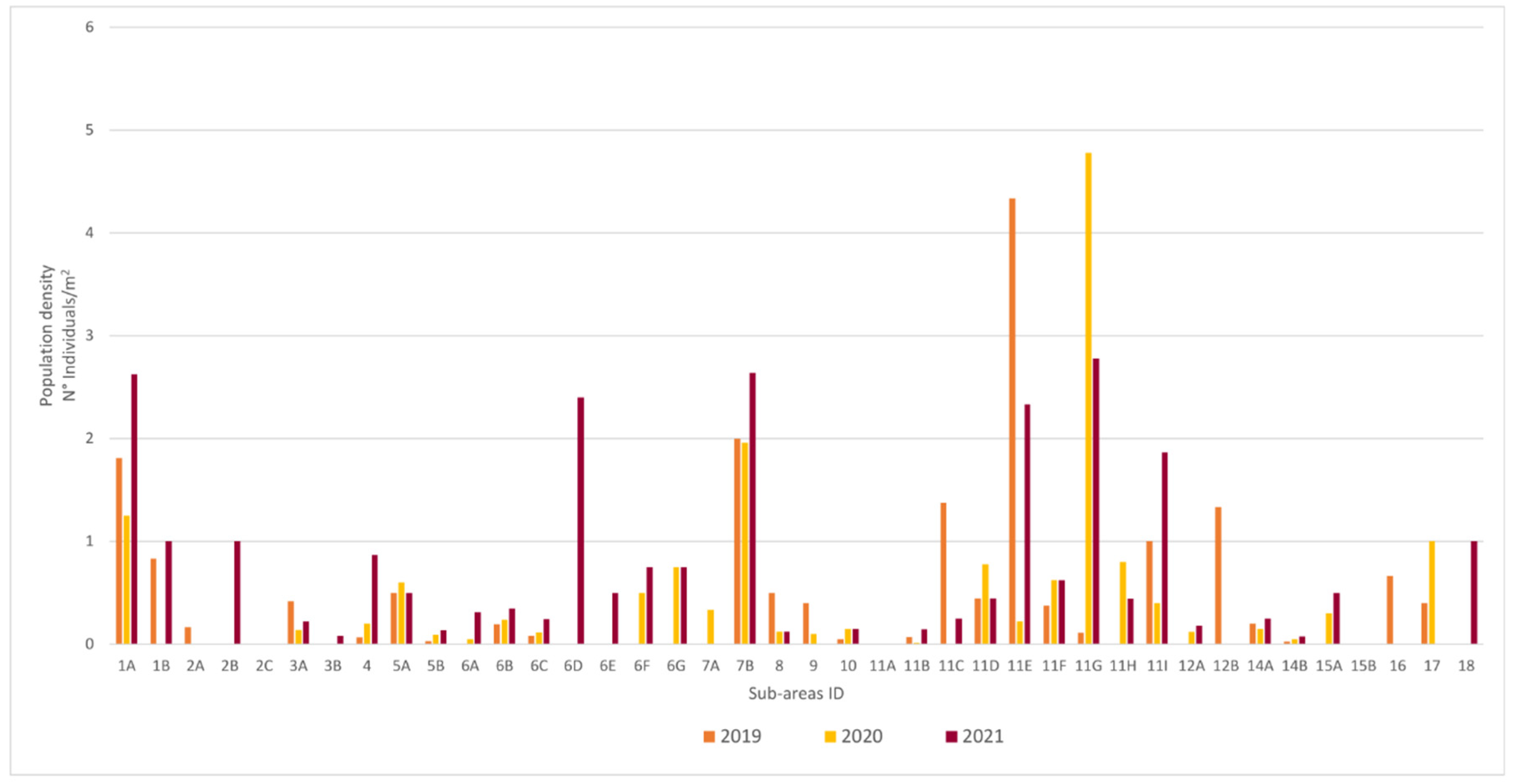
3.1. Population Structure

The census (Table S1) showed that the population of S. ceratophylloides is currently fragmented into 17 micro-populations (census 2021), subdivided into 40 sub-areas, each consisting of 1 individual up to a maximum of 401, for a grand total of 1555 plants.

The number of individuals present in each sub-area was not constant over time. As shown in Figure 4, there were more numerous micro-populations with >60 individuals (5B, 6A, 6B, 6C, 7B, 10) that showed an increasing trend. Conversely the less numerous micro-populations with >20 individuals (1A, 1B, 2A, 3A, 4, 5A, 11B, 11C, 11D, 11E, 11F, 11G, 11H, 11I, 12A, 14A, 15A, 16, 17) were more fluctuating, as were those with a small number of individuals >10 (2B, 2C, 3B, 6D,6E, 6F, 6G, 7A, 8, 9, 11A, 12B, 15B, 18). For the population 6G, the rate of increase/decrease was calculated with reference to the years 2020–2021 as the sub-area did not exist before. Moreover, this sub-area maintained a constant number of individuals over the two years. Sub-area 2C, on the other hand, was extinct, as no individuals were recorded in 2021.

The total number of individuals for each sub-area in the three different years ranged from a minimum of 1 to a maximum of 272 in 2019, for a total of 1242 individuals, from 1 to 348 in 2020, for a total of 1317 individuals, and from a minimum of 1 to a maximum of 401 in 2021 (Table S1). The distribution of the different “life stages” also varied from year to year. “Life stage” S represented 1% of the population and remained constant in all three survey years. “Life stage” JI constituted 5% of the individuals surveyed in 2019 and 2020, while in 2021 it represented 10 % of the individuals with an increase of 5%. “Life stage” V increased gradually year on year, from 20% in 2019, to 25% in 2020, to 31% in 2021. The more generative “life stages” SG and LG tended to decrease over time: SG in 2019 represented 43% of the population, in 2020 39% and in 2021 37%, while LG was 31% in 2019, 30% in 2020, and 21% in 2021 (Figure 5).

To confirm the previous results, the population density was estimated in relation to total individuals, distinguishing them as non-breeding and breeding individuals in the 3 different years in relation to the areas considered for each sub-area (Table S1).

The graph (Figure 6) shows that the different sub-areas had different population densities in different years. Some of the sub-areas showed an increasing trend (1A, 2B, 4, 5A, 5B, 6A, 6B, 6C, 6E, 6F, 7A, 7B, 10, 11A, 11B, 11I, 12A, 14A, 14B, 18), others showed a decreasing trend (1B, 2A, 2C, 3A, 3B, 8, 9, 11C, 12B, 17) and some had strong fluctuations from year to year, being those most directly impacted by human activities (6D,11E, 11F, 11G,11H,15A, 15B, 16). Sub-area 6G (discovered in 2020) was constant over the years.

The graph of average numbers of individuals/area of the sub-areas over the three years (Figure 7) shows that as the area increased, the number of individuals increased, with a maximum of 340 individuals over an area of 1200 m² in sub-area 5B.

Analysing the variations in the density of non-breeding individuals over the three years (Figure 8) showed extreme variability. Only in a few micro-populations was a constant density observed (1A, 3A, 5A, 5B, 7B, 11D, 11F, 14A, 14B). In many sub-areas, years in which non-breeding individuals were not present alternated with years in which they suddenly appeared (1B, 2A, 2B, 3B, 4, 6A, 6D, 6E, 7A, 11C, 11E, 11G, 12B, 16, 17, 18). Non-breeding individuals were not present in sub-areas 2C, 11A AND 15B.

On the other hand, if we consider the variation in density of breeding individuals over the three years (Figure 9), we can observe that in many sub-areas there was a limited fluctuation in density (1A, 1B, 2A, 2B, 3A, 3B, 4, 5A, 5B, 6A, 6B, 6C, 6D, 6E, 6F, 7A, 7B, 8, 9, 10, 11A, 11B, 11C, 11G, 11I, 12A, 12B, 14A, 14B, 17, 18), while in some sub-areas (2C, 11D, 11E, 11F, 11H, 15A, 15B, 16) a strong fluctuation was observed, similar to what was observed for the total density.

The cluster analysis of the “life stage”/number of individuals matrix highlighted the dissimilarity between different sub-areas. This aggregation revealed three groups of population types (Figure 10 and Figure 11). To define the significance of the three different groups, the ratio of non-breeding juvenile stages to breeding adult stages was taken into account [(S + JI + V)/G], with G = (SG + LG).

The sub-areas of the first group were clearly distinct from the others and could be defined as “Dynamic”, in accordance with [11], as they were characterised by a higher number of non-breeding juveniles than breeding ones. In fact, this group was characterised by a relatively high [(S + JI + V)/G] ratio, with an average of 2.91 and a range of 1.25 to 5.75. The average of young individuals was 71.1%, of which 46.6% were represented by “life stage” V, 19.9% by JI and 4.6% by S (Figure 11).

The second group was characterised by sub-areas with fewer non-breeding juveniles than the previous group, and instead had a higher number of breeding individuals. The ratio [(S + JI + V)/G] averaged 0.49 and ranged from 0.27 to 0.79. “Life stages” were represented by 32.1% non-breeding individuals and 67.9% breeding individuals, of which 45.6% belonged to “life stage” SG. This group could be defined as “Normal” or “Stable” according to [60] (Figure 11).

The third group was represented by aged sub-areas, characterised by a higher presence of SG and LG breeding individuals, corresponding to 83.1% of the entire population, of which the majority belonged to the “life stage” LG (58%). Very few young non-breeding individuals were present in this group, making up 16.9% of all the sub-areas, of which 14.7% belonged to “life stage” V, 1.9% J-I and only 0.3% from S. The ratio [(S + JI + V)/G] had an average value of 0.21 and ranged from 0.07 to 0.30. In relation to the analysed factors, this group could be defined as “Regressive” in accordance with [60] (Figure 11).

Overall, “Regressive” populations accounted for 40% of the entire population, while “Normals” made up only 36% and “Dynamics” 24%.

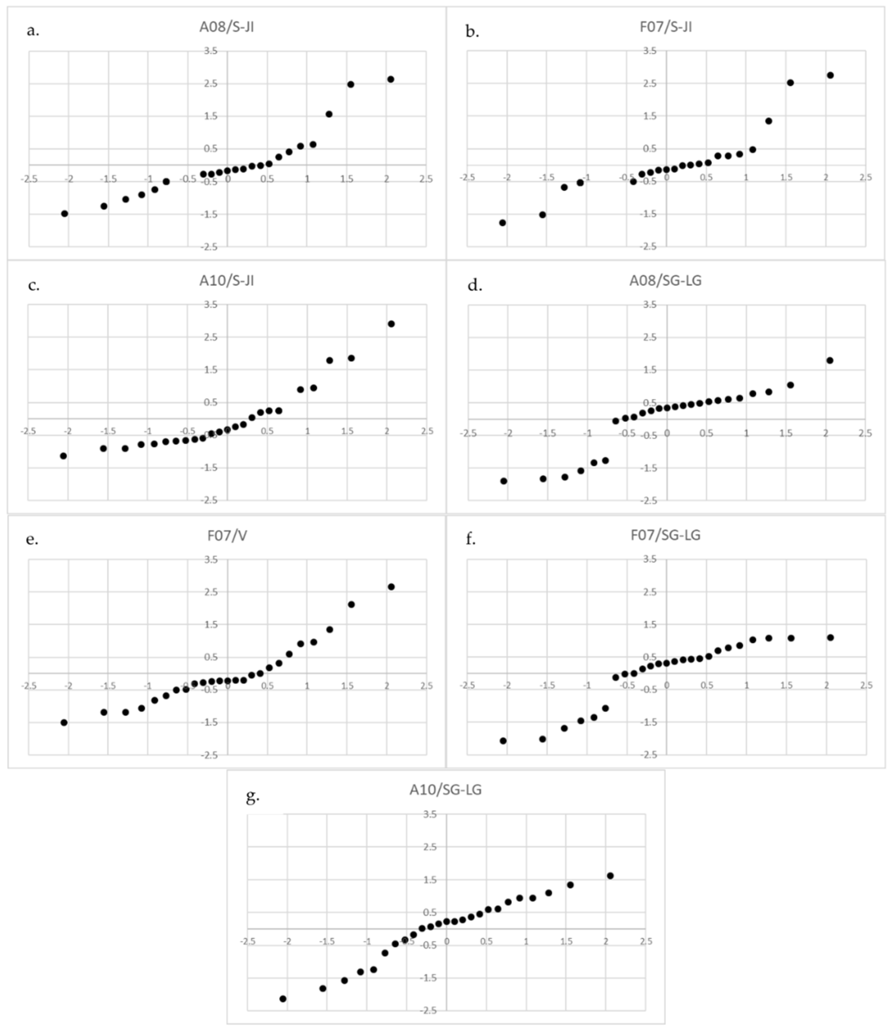
3.2. Relationships between “Life Stages” and Pressures

The field surveys made it possible to determine the pressure factors and the intensity with which they affected the different sub-areas of the S. ceratophylloides population (Table S4), detailed in

Table 2. Pressures observed on the population of Salvia ceratophylloides Ard. The abbreviations of the sub-areas refer to Table S1. The intensity of the pressures is expressed in H = high; M = medium; L = low.

Sub Aree		1A	6B	7B	11E	11G	11I	3A	4	5B	9	11B	11C	11D	11F	11H	3B	5A	6A	6C	6E	8	12A	14A	14B	17
Population Tipe		Dynamic						Normal									Regressive
Threats Code	Threats Name
A08	Mowing or cutting of grasslands				L	L	L				L	L	L	L	L	L						L	L
A10	Extensive grazing or undergrazing by livestock							L		L							L	L						M	M
A11	Burning for agriculture	H																						L	L
A15	Tillage practices in agriculture			H														L			M			L	L	M
F07	Sports, tourism and leisure activities				H	H	H					H	H	H	H	H
I01-I02	Invasive alien species of Union/not Union concern	M	M		L	L						L	L	L	L	M				L			H	L	M	L
L06	Interspecific faunal and floral relations (competition, predation, parasitism, pathogens)	H	H	H	M			M			M	M					M		H	H		H	H	M	M	L
M05	Collapse of terrain, landslide																L

.

Linear regression analysis showed the effect of pressures acting in sub-areas in relation to different “life stages” (

Table 3. Linear regression analysis between “life stage” and pressure (R²—correlation value; p—level of significance).

Life Stage	Threats	R2	p	Sign.
S-JI	A08	0.434	0.03	**
	F07	0.576	0.003	**
	A10	−0.403	0.046	**
V	F07	0.352	0.08	*
SG-LG	A08	−0.343	0.09	*
	F07	−0.523	0.01	**
	A10	0.395	0.05	*

p ≤ 0.1, * < 0.05, ** < 0.01.

). The youngest “life stages” S-JI were positively correlated with mowing and recreational tourism activities (A08 R² = 0.43, p = 0.03; F07 R² = 0.58, p = 0.003) and negatively with grazing (A10 R² = −0.40, p = 0.05). Vegetative stages V were positively correlated with recreational tourism activities (F07 R² = 0.352, p = 0.08). Breeding “life stages” SG-LG were positively correlated with grazing (A10 R² = 0.395, p = 0.05) and negatively with mowing (A08 R² = 0.395, p = 0.05).

The Q-Q plot (Quantiles-Quantiles graph) graphically demonstrated an effective normal distribution of the data, validating the hypotheses obtained from the linear regression analysis, as shown in Figure 12.

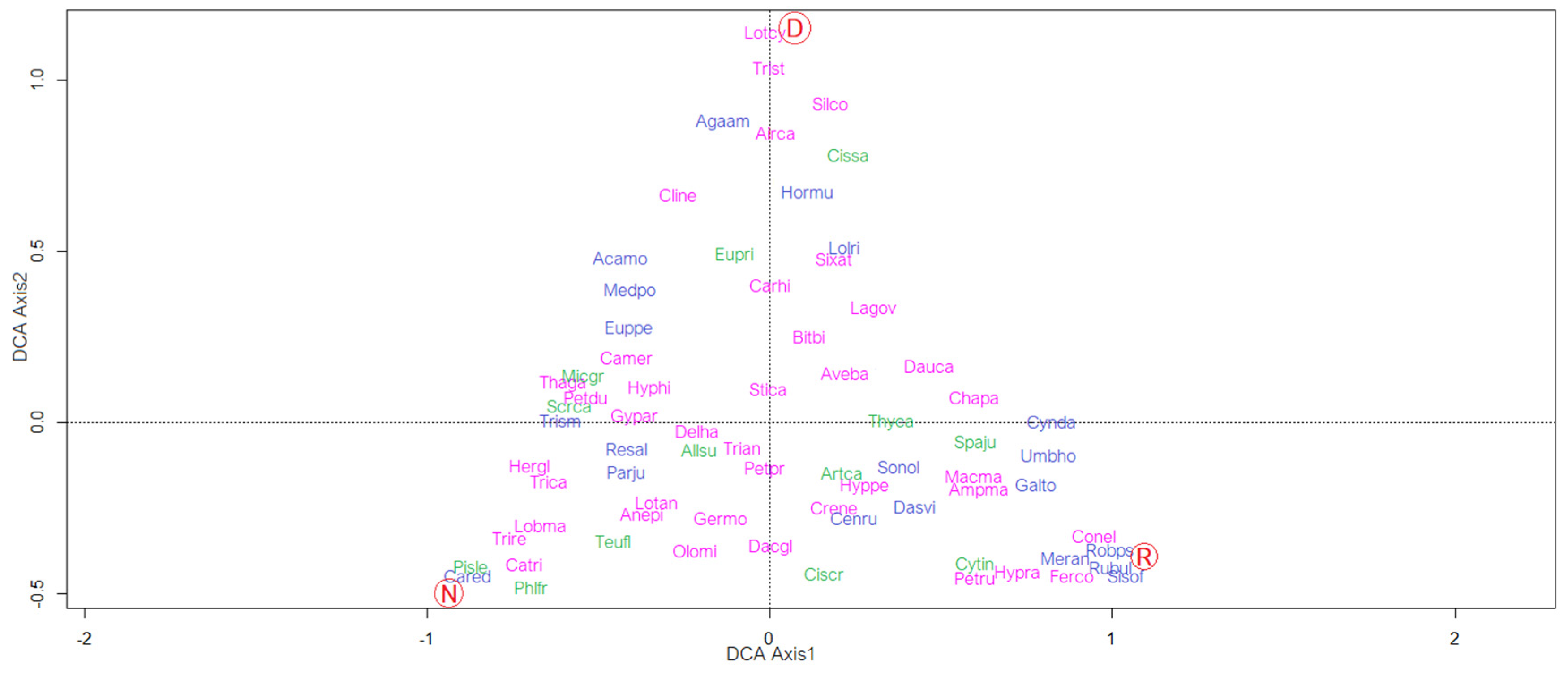
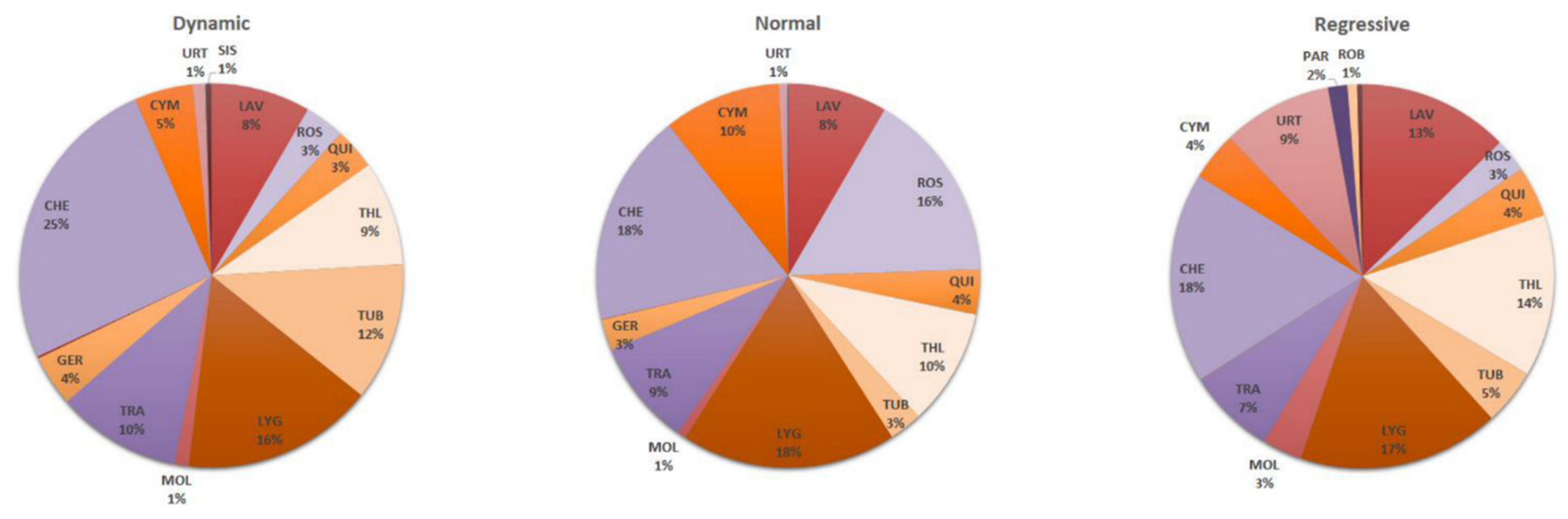
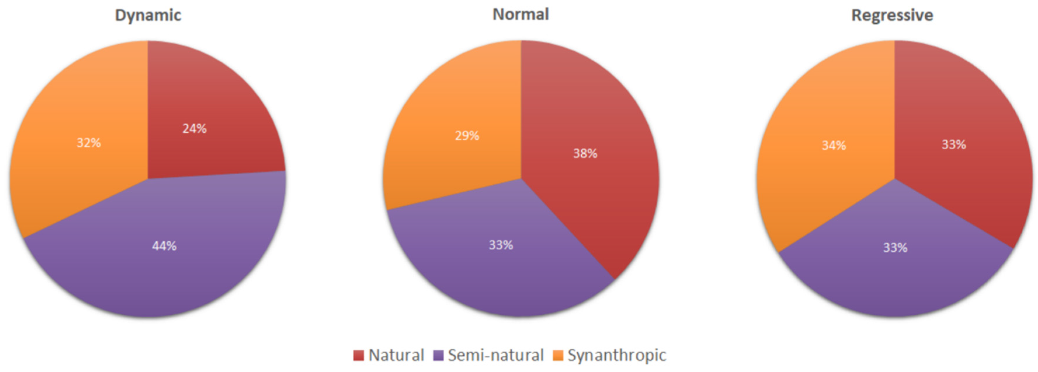
3.3. Relationships between “Life Stage” and Vegetation

The relationship between three different population types, resulting from the cluster analysis and the vegetation surveyed with the phytosociological methodology, was examined using DCA (Figure 13). The geometric distance on the diagram reflects the difference between the surveys. Examining the positions of the species on the diagram in relation to the 3 different population groups resulting from the previous analyses (“Dynamic”, “Normal”, “Regressive”) we can see some significant differences. The Eigenvalues for the four axes of the DCA were 0.808, 0.604, 0.341 and 0.219, respectively. Since Jongman et al. [62] believe that axes with Eigenvalue values less than 0.5 should not be considered, as they do not express a relevant floristic gradient, only the first axis (DCA Axis1) and the second (DCA Axis2) can be considered representative of the main floristic gradient.

The number of species is higher in the “Normal” populations, ranging from a minimum of 17 to a maximum of 70, with an average of 43 species in all the sub-areas examined. The “Dynamic” populations presented a minimum of 15 and a maximum of 60 species, with an average value of 42.5. Species in the “Regressive” populations were scarcely numerous, with a minimum of 18 and a maximum of 34, the mean value being 28 species (

Table 4. Maximum and minimum number of species present in the surveys of the different types of populations of Salvia ceratophylloides Ard. (“Normal”, “Dynamic”, “Regressive”).

Population Typology	Min. Species	Max. Species	Mean
Normal	17	70	43
Dynamic	15	60	42.5
Regressive	18	34	28

).

Anemone hortensis L. subsp. hortensis, Arenaria leptoclados (Rchb.) Guss. subsp. leptoclados, Asparagus acutifolius L., Asparagus albus L., Eudianthe coeli-rosa (L.) Fenzl ex Endl., Euphorbia peplus L., Hippocrepis ciliata Willd., Lysimachia arvensis (L.) U.Manns & Anderb. subsp. arvensis, Orchis italica Poir., Petrosedum tenuifolium (Sm.) Grulich, Plantago albicans L., Poa trivialis L., Rumex bucephalophorus L. subsp. bucephalophorus, Senecio leucanthemifolius Poir., Trigonella italica (L.) Coulot & Rabaute, Verbena officinalis L. are only present in “Dynamic” populations.

Rumex pulcher L., Seseli tortuosum L. subsp. tortuosum, Andropogon distachyos L., Echium vulgare L. subsp. pustulatum (Sm.) Em. Schmid & Gams, Linaria purpurea L., Onopordum illyricum L. subsp. illyricum, Pteridium aquilinum (L.) Kuhn subsp. aquilinum, Scolymus hispanicus L., Silene gallica L., Solanum nigrum L., Verbascum thapsus L. subsp. thapsus, Vinca major L. subsp. major, Viola odorata L. are exclusive to “Natural” populations.

Ailanthus altissima (Mill.) Swingle, Anredera cordifolia (Ten.) Steenis, Brassica fruticulosa Cirillo subsp. fruticulosa, Calendula arvensis (Vaill.) L., Convolvulus althaeoides L., Lolium perenne L., Oloptum thomasii (Duby) Banfi & Galasso, Plantago lanceolata L., Silene vulgaris (Moench) Garcke subsp. tenoreana (Colla) Soldano & F.Conti, Crupina crupinastrum (Moris) Vis., Jasione montana L., Papaver rhoeas L., Opuntia ficus-indica (L.) Mill. are exclusive to “Regressive” populations.

The taxa present in the vegetation surveys belonged to 16 phytosociological classes. Of these, 4 brought together vegetation from natural habitats, 5 semi-natural, 7 synanthropic (Tables S2 and S3).

In relation to the phytosociological classes, the populations showed a different distribution (Figure 14). The class Chenopodietea was the most represented, with a coverage value of 25% in the “Dynamic”, 18% in the “Normal” and 18% in the “Regressive” populations.

The other most represented classes were the following: Lygeo sparti-Stipetea tenacissimae, with a coverage value of 16% in the “Dynamic”, 18% in the “Normal” and 17% in the “Regressive” populations; Cisto-Lavanduletea stoechadis, with a coverage value of 8% in the “Dynamic” and “Normal” populations and 13% in the “Regressive” populations; Thlaspietea rotundifoliae, with a coverage value of 8% in the “Dynamic” and “Normal” populations and 14% in the “Regressive” populations; Galio aparines-Urticetea dioicae, with a cover value of 6% in “Dynamic” populations, 10% in “Normal” populations and 13% in “Regressive” populations; Stipo-Trachynietea distachyae, with a cover value of 7% in” Dynamic” populations, 8% in “Normal” populations and 5% in “Regressive” populations. The other phytosociological classes had very low coverage values, and, in particular, the species of the class Helianthemetea guttati presented a coverage value of 12% for the “Dynamic” populations, while having very low values for the “Normal” (3%) and “Regressive” (5%) populations. Species of the class Ononido-Rosmarinetea, had higher cover values in “Normal” populations (16%) while they were sporadic in “Dynamic” and “Regressive” populations. Alien species of the class Robinietea were scarcely present (1%) only in the “Regressive” populations.

Taking into consideration the habitats (natural, semi-natural and synanthropic) to which the vegetation classes refer (Figure 15), it can be seen that the “Dynamic” populations presented a greater number of species linked to semi-natural habitats (44%) and synanthropic species (32%). The “Normal” populations predominantly presented species typical of natural habitats (38%), with fewer species linked to semi-natural habitats (33%) and synanthropic species (29%). Regarding the “Regressive” populations, the species belonging to the three habitats were distributed almost equally.

4. Discussion

The census revealed that the population of S. ceratophylloides showed an inconstant trend over time, with significant differences in the number of individuals present in the different populations (Figure 4). The more structured populations, with a greater number of individuals, tended to grow over the years, as evidenced by the positive values of the Malthus index [49] (5B, 6B, 6C, 7B, 10). This increase was due to the better organised structure of the population itself, and its ability to resist external influences that may affect its dynamics. Populations with fewer individuals, on the other hand, tended to be more sensitive to external influences that caused their decrease: this was highlighted by the negative value of the Malthus index [49] (2A, 8, 9, 15, 17).

The trend of the census population in the 40 sub-areas from 2019 to 2021 (Figure 4), also showed considerable differences in the rate of increase–decrease: in fact, in some of the sub-areas there was a strong variation, due to the fact that some micro-populations had been subjected to very strong external pressures, such as fire or mowing.

The analysis of the “life stages” of the entire population (Figure 5) showed that non-breeding “life stages” (S, JI, V) represented the lowest percentage of the population, varying from 26% in 2019, to 31% in 2020, up to 42% in 2021, showing an overall increasing trend. In contrast, the reproductive “life stages” represented more than 50% of the population and underwent a significant decrease over the three years. The increase and decrease in “life stages” was directly related to the pressures the habitat underwent, with these pressures acting more violently on the more advanced “life stages” and being less influential in the juvenile stages (Table 3).

The cluster analysis of the matrix No. of individuals/“life stage”/sub-area, made it possible to distinguish, in accordance with Heglad [11] and Oostermeijer [60], three different types of populations in relation to the distribution of the different “life stages”, defined as: “Dynamic”, “Normal”, “Regressive” (Figure 10). “Regressive” populations accounted for 40% of the entire population, while “Normal” constituted 36% and “Dynamic” 24%. Non-breeding “life stages” (S, JI, V) were more represented in the “Dynamic” populations, which were characterised by a high ratio of non-breeding individuals to breeding individuals (SG, LG) (Figure 11). In the “Normal” populations, a balance between breeding and non-breeding “life stages” was observed, while in the “Regressive” populations there was a greater representation of non-breeding “life stages”, represented mainly by “life stage” LG, an indication of the ageing of the population.

The pressures affecting the population and the individual sub-areas in which it was distributed (Table S4) were, first and foremost, the fires that often affect this area [63,64], mostly linked to grazing or agricultural activities, which, if repeated over time, can lead to the extinction of S. ceratophylloides populations, as observed for micro-population 13 [61]. Alien invasive species, both included and not included in EU Directive 1143/2014, were often introduced accidentally (micro-population 12) or deliberately (micro-population 11), with serious negative consequences for the invaded habitat [21,22,23,24]. Salvia ceratophylloides was severely damaged by various pests that affect fruits and stems. Squamapion elongatum (Germar, 1817) (Coleoptera-Apionidae) digs tunnels into the stems, inhibiting plant growth and subsequent flower formation. Systole salvia (Zerova 1970) (Hymenoptera-Eurytomidae) irreparably damages the fruits, as the larva of this species feeds on them, emptying them completely [65].

The pressures analysed affected the different “life stages” differently (Table 3) and, consequently, the different types of population. In particular, the non-breeding “life stages” (S, JI, V), that characterised the “Dynamic” populations, were positively correlated with anthropic activities, such as mowing and sporting, tourist and recreational activities. These pressures tended, on the other hand, to negatively influence the breeding “life stages” (SG, LG), thus affecting, above all, the “Regressive” populations. Mowing damages adult individuals, often represented by large branched plants 0.5–1 m high, while avoiding very young individuals (S, JI), which grow close to the ground (Figure 3). Although the species was not eaten by animals, due to the presence of essential oils [66], young individuals were negatively affected by the presence of grazing [67]. Trampling caused by ungulates [Capra hircus (L., 1758) and Ovis aries (L., 1758)], irreparably damages the seedlings. On the contrary, the latter was positively correlated with “life stage” SG, LG to which it did not cause damage, instead limiting competition with other pabular species eaten by grazing animals.

There are also many threats acting in the areas surrounding the population, which could affect the species’ habitats. Urban expansion of cities, with the consequent construction of infrastructure (E01, F01) is one of the main threats as it is a factor in the fragmentation and change of natural and semi-natural habitats [68,69,70], as highlighted by Spampinato et al. [71,72]. Urbanisation has already, in the past, caused the extinction of several micro-populations (19, 20, 21) of the species known from the literature (Figure 2) [39]. Reforestations carried out mainly in the 1950s (B01) [73,74] contributed to the extinction of other populations (22, 23) reported in the literature (Figure 2) [40]. Studies on the eco-physiological characteristics of the species [66] show that climate change [16] may adversely affect the species’ population. On the whole, all the sub-areas suffered mainly from anthropogenic pressures, which, as shown, acted by altering the relationships between the different life stages. Under conditions of less anthropic disturbance, the population structure was ‘normal’ with a more or less balanced ratio of breeding individuals to nonbreeding individuals. Under more natural conditions of less anthropogenic disturbance, the latter was probably the population structure of S. ceratophylloides. The DCA analysis of the species/population type matrix (Figure 13) showed that the different species detected in the vegetation analysis did not follow a defined trend: in fact synanthropic, natural and semi-natural species, in relation to the different types of populations obtained from the cluster analysis (“Normal”, “Dynamic”, “Regressive”), on the whole were distributed in a way that did not involve making groups. It was observed, however, that some of them were more closely linked to certain population types. In particular, the “Regressive” (R) populations were characterised by a greater presence of synanthropic and ruderal species (Robinia pseudoacacia L., Rubus ulmifolius Schott, Sisymbrium officinale (L.) Scop., Mercurialis annua L., Galactites tomentosus Moench, Dasypyrum villosum (L.) P.Candargy, Centranthus ruber (L.) DC. subsp. ruber, Sonchus oleraceus L., Umbilicus horizontalis (Guss.) DC., Cynodon dactylon (L.) Pers.), frequent in heavily disturbed habitats. The “Dynamic” (D) populations, on the other hand, presented numerous semi-natural species (Lotus cytisoides L., Trifolium stellatum L., Silene colorata Poir., Aira caryophyllea L., Sixalix atropurpurea (L.) Greuter & Burdet, Lagurus ovatus L. subsp. ovatus). The “Normal” (N) populations showed an equal distribution of the different species types, with greater representation of natural habitat species (Pistacia lentiscus L., Phlomis fruticosa L., Teucrium flavum L. subsp. flavum).

Heglad et al. [11], in their analysis of the related Salvia pratensis, analysed the populations in relation to the different management methods (mowing or grazing) and showed how these significantly influence the vegetation of the different population types (“Regressive”, “Dynamic” and “Normal”). They clearly distinguish groups of species related by ecological characteristics (nutrient-poor or nutrient-rich soil species) from the different population types.

Shomurodov et al. [6] stated that populations of Salvia lilacinocoerulea Nevski, endemic and punctiform species to the Western Pamir-Alay mountain range, are strongly conditioned by vegetation and soil type. These two factors, strongly affect the population dynamics, in some cases representing a real limitation for the species. In our study, these factors did not influence the population, essentially because the pedology was the same in all sub-areas. The analysis of the vegetation classes (Figure 14) showed that the species of the class Chenopodietea were widely distributed in all the population types, bearing witness to the anthropic disturbance affecting them. The class Lygeo sparti-Stipetea tenacissimae was also widespread in all population types, i.e., in arid environments of the Mediterranean belt, influenced by fires and characterised by herbaceous perennials, such as Hyparrhenia hirta (L.) Stapf subsp. hirta and Ampelodesmos mauritanicus (Poir.) T.Durand & Schinz. In the “Normal” populations, the species of the garrigues, typical of the classes Cisto-Lavanduletea stoechadis and Ononido-Rosmarinetea, were better represented, while in the “Regressive” populations the species of the latter classes were poorly represented, and the species linked to synanthropic environments, such as those characteristic of the classes Galio aparines-Urticetea maioris, Papaveretea rhoeadis and Robinietea, were better represented.

Overall, a certain relationship was observed between the characteristic species of the various vegetation classes (natural, semi-natural, synanthropic) and the population types (“Regressive”,” Dynamic”, “Normal”) (Figure 15). In particular, species typical of the natural type classes were well represented in the “Normal” populations, while species typical of the semi-natural vegetation classes were better represented in the “Dynamic” type populations and, finally, albeit slightly, species typical of the synanthropic vegetation classes were better represented in the “Regressive” type populations.

Numerous studies have dealt with threatened and/or endangered species [4,5,6]. These studies focused on population dynamics, in order to establish safeguards and protection measures for these species. This can be achieved through specific in situ conservation measures, such as the establishment of micro-reserves [75], an approach successfully developed in recent decades in Spain and, subsequently, in other European and Mediterranean countries [76,77,78]. For S. ceratophylloides, the extension of the micro-reserve should cover about 7 km², around the hills of Reggio Calabria, encompassing the entire Area Of Occurrence (AOO) of the species [48].

5. Conclusions

This work lays the scientific basis for the planning of conservation and protection measures capable of reducing and eliminating, over time, the pressures that adversely affect the Salvia ceratophylloides population.

The work shows that S. ceratophylloides micro-populations have non-stable dynamics over time, and are deeply conditioned by the pressures exerted on the habitat and on individuals, acting with different intensity in relation to different “life stages”. These stresses are mostly represented by anthropogenic disturbances, which affect habitat quality and are reflected in population dynamics over time. Important also are the pressures of natural origin that affect the reproductive and regenerative capacities of the species. The reiteration of such pressures over time could lead to slow and ineluctable decline and, thus, extinction of S. ceratophylloides in the wild. This would primarily affect micro-populations with a small number of individuals of the order of a dozen or less, which, as evidenced by the Malthus index, show a decrease. It is therefore on these micro-populations, composed of a limited number of individuals, that action needs to be taken to reduce impacts and favour the renovation of the species, including through reintroduction. This can be achieved through specific in situ conservation measures, such as the establishment of micro-reserves. However, possible ex situ conservation measures at germplasm banks and botanical gardens should not be ruled out, nor the dissemination of this species in private gardens.

References

1. Hutchings, M.J. Monitoring plant populations: Census as an aid to conservation. In Monitoring for Conservation and Ecology; Goldsmith, F.B., Ed.; Chapman & Hall: London, UK, 1991; pp. 61–76. [Google Scholar]
2. Oostermeijer, J.G.B.; Brugman, M.L.; de Boer, E.R.; den Nijs, J.C.M. Temporal and spatial variation in the demography of Gentiana pneumonanthe, a rare perennial herb. J. Ecol. 1996, 84, 153–166. [Google Scholar] [CrossRef]
3. Menges, E.S. Population viability analyses in plants: Challenges and opportunities. Trends Ecol. Evol. 2000, 15, 51–56. [Google Scholar] [CrossRef]
4. Aikens, M.L.; Roach, D.A. Population dynamics in central and edge populations of a narrowly endemic plant. Ecology 2014, 95, 1850–1860. [Google Scholar] [CrossRef] [PubMed]
5. Shaltout, K.H.; Ahmed, D.A.; Hatem, A. Shabana, Population structure and dynamics of the endemic species Phlomis aurea Decne in different habitats in southern Sinai Peninsula, Egypt. Glob. Ecol. Conserv. 2015, 4, 505–515. [Google Scholar] [CrossRef]
6. Shomurodov, H.F.; Khuzhanazarov, U.E.; Beshko, N.Y.; Akhmadalieva, B.; Sharipova, V.K.A. Demographic structure of populations of Salvia lilacinocoerulea Nevski, a rare species endemic to the Western Pamir-Alay (Uzbekistan, Turkmenistan). Am. J. Plant Sci. 2017, 8, 1411. [Google Scholar]
7. Hoekstra, J.M.; Boucher, T.M.; Ricketts, T.H.; Roberts, C. Confronting a biome crisis: Global disparities of habitat loss and protection. Ecol. Lett. 2005, 8, 23–29. [Google Scholar] [CrossRef]
8. Schemske, D.W.; Husband, B.C.; Ruckelshaus, M.H.; Goodwillie, C.; Parker, I.M.; Bishop, J.G. Evaluating Approaches to the Conservation of Rare and Endangered Plants. Ecology 1994, 75, 585–606. [Google Scholar] [CrossRef]
9. Menges, E.S. Evaluating extinction risks in plant populations. In Conservation Biology for the Coming Decade; Fiedler, P.L., Jain, S.K., Eds.; Chapman & Hall: New York, NY, USA, 1998; pp. 49–65. [Google Scholar]
10. Harvey, H.J. Population biology and the conservation of rare species. In Studies on Plant Demography: A Festschrift for John L. Harper; White, J., Ed.; Academic Press: London, UK, 1985; pp. 111–123. [Google Scholar]
11. Hegland, S.J.; Van Leeuwen, M.; Oostermeijer, J.G.B. Population structure of Salvia pratensis in relation to vegetation and management of Dutch dry floodplain grasslands. J. Appl. Ecol. 2001, 38, 1277–1289. [Google Scholar] [CrossRef]
12. Thuiller, W.; Lavorel, S.; Araújo, M.B.; Sykes, M.T.; Prentice, I.C. Climate change threats to plant diversity in Europe. Proc. Natl. Acad. Sci. USA 2005, 102, 8245–8250. [Google Scholar]
13. Walther, G.R.; Post, E.; Convey, P.; Menzel, A.; Parmesan, C.; Beebee, T.J.; Fromentin, J.M.; Hoegh-Guldberg, O.; Bairlein, F. Ecological responses to recent climate change. Nature 2002, 416, 389. [Google Scholar] [CrossRef]
14. Jump, A.S.; Penuelas, J. Running to stand still: Adaptation and the response of plants to rapid climate change. Ecol. Lett. 2005, 8, 1010–1020. [Google Scholar] [CrossRef] [PubMed]
15. Del Río, S.; Canas, R.; Cano, E.; Cano-Ortiz, A.; Musarella, C.; Pinto-Gomes, C.; Penas, A. Modelling the impacts of climate change on habitat suitability and vulnerability in deciduous forests in Spain. Ecol. Indic. 2021, 131, 108202. [Google Scholar] [CrossRef]
16. Intergovernmental Panel on Climate Change (IPCC). Climate Change 2022: Mitigation of Climate Change. In Contribution of Working Group III to the Sixth Assessment Report of the Intergovernmental Panel on Climate Change; Shukla, P.R., Skea, J., Slade, R., al Khourdajie, A., van Diemen, R., McCollum, D., Pathak, M., Some, S., Vyas, P., Fradera, R., et al., Eds.; Cambridge University Press: Cambridge, UK; New York, NY, USA, 2022. [Google Scholar]
17. Vié, J.C.; Hilton-Taylor, C.; Stuart, S.N. (Eds.) Wildite in a Changing Word—An Analysis of the 2008 /UN Red List of Threatened Species; IUCN: Gland, Switzerland, 2009; p. 180. [Google Scholar]
18. Içik, K. Rare and endemic species: Why are they prone to extinction? Turk. J. Bot. 2011, 35, 411–417. [Google Scholar]
19. Spampinato, G.; Laface, V.L.A.; Ortiz, A.C.; Canas, R.Q.; Musarella, C.M. Salvia ceratophylloides Ard. (Lamiaceae): A rare endemic species of Calabria (Southern Italy). In Endemic Species; Cano Carmona, E., Musarella, C.M., Cano Ortiz, A., Eds.; IntechOpen: London, UK, 2019. [Google Scholar] [CrossRef]
20. Fenu, G.; Ferretti, G.; Gennai, M.; Lahora, A.; Mendoza-Fernández, A.J.; Mota, J.; Robles, J.; Serra, L.; Schwarzer, H.; Sánchez-Gómez, P.; et al. Global and Regional IUCN Red List Assessments: 4. Ital. Bot. 2017, 4, 61–71. [Google Scholar] [CrossRef]
21. Thuiller, W.; Richardson, D.M.; Midgley, G.F. Will Climate Change Promote Alien Plant Invasions? Springer: Berlin/Heidelberg, Germany, 2008; pp. 197–211. [Google Scholar]
22. Laface, V.L.A.; Musarella, C.M.; Cano Ortiz, A.; Quinto Canas, R.; Cannavò, S.; Spampinato, G. Three new alien taxa for Europe and a chorological update on the alien vascular flora of Calabria (Southern Italy). Plants 2020, 9, 1181. [Google Scholar] [CrossRef]
23. Musarella, C.M.; Stinca, A.; Cano-Ortíz, A.; Laface, V.L.A.; Petrilli, R.; Esposito, A.; Spampinato, G. New data on the alien vascular flora of Calabria (Southern Italy). Ann. Bot. 2020, 10, 55–66. [Google Scholar] [CrossRef]
24. Spampinato, G.; Laface, V.L.A.; Posillipo, G.; Cano Ortiz, A.; Quinto Canas, R.; Musarella, C.M. Alien flora in Calabria (Southern Italy): An updated checklist. Biol. Invasions 2022, 24, 2323–2334. [Google Scholar] [CrossRef]
25. Perrino, E.V.; Valerio, F.; Jallali, S.; Trani, A.; Mezzapesa, G.N. Ecological and biological properties of Satureja cuneifolia Ten. and Thymus spinulosus Ten.: Two wild officinal species of conservation concern in Apulia (Italy). A preliminary survey. Plants 2021, 10, 1952. [Google Scholar] [CrossRef]
26. Valerio, F.; Mezzapesa, G.N.; Ghannouchi, A.; Mondelli, D.; Logrieco, A.F.; Perrino, E.V. Characterization and antimicrobial properties of essential oils from four wild taxa of Lamiaceae family growing in Apulia. Agronomy 2021, 11, 1431. [Google Scholar] [CrossRef]
27. Zhao, F.; Chen, Y.P.; Salmaki, Y.; Drew, B.T.; Wilson, T.C.; Scheen, A.C.; Celep, F.; Bräuchler, C.; Bendiksby, M.; Wang, Q.; et al. An updated tribal classification of Lamiaceae based on plastome phylogenomics. BMC Biol. 2021, 19, 2. [Google Scholar] [CrossRef]
28. Walker, J.B.; Sytsma, K.J.; Treutlein, J.; Wink, M. Salvia (Lamiaceae) is not monophyletic: Implications for the systematics, radiation, and ecological specializations of Salvia and tribe Mentheae. Am. J. Bot. 2004, 91, 1115–1125. [Google Scholar] [CrossRef] [PubMed]
29. Kintzios, S.E. Sage—The Genus Salvia; CRC Press: Boca Raton, FL, USA, 2003; p. 318. [Google Scholar]
30. Askari, S.F.; Avan, R.; Tayarani-Najaran, Z.; Sahebkar, A.; Eghbali, S. Iranian Salvia species: A phytochemical and pharmacological update. Phytochemistry 2021, 183, 112619. [Google Scholar] [CrossRef] [PubMed]
31. Hedge, I.C. Salvia L. Flora Europaea; Tutin, T.G., Heywood, V.H., Burges, N.A., Moore, D.M., Valentine, D.H., Walters, S.M., Webb, D.A., Eds.; Cambridge University Press: Cambridge, UK, 1972; Volume 3, pp. 188–192. [Google Scholar]
32. Nikolova, M.; Aneva, I.Y. European Species of Genus Salvia: Distribution, Chemodiversity and Biological Activity. Salvia Biotechnol. 2017, 1–30. [Google Scholar] [CrossRef]
33. Portal to the Flora of Italy. Available online: http:/dryades.units.it/floritaly (accessed on 21 June 2022).
34. Pignatti, S. Flora d’Italia; Edagricole: Bologna, Italy, 1982; Volume 2, pp. 502–507. [Google Scholar]
35. Pignatti, S. Flora d’Italia, 2nd ed.; Edagricole: Bologna, Italy, 2018; Volume 3, pp. 301–310. [Google Scholar]
36. Del Carratore, F.; Garbari, F. Indagini Biosistematiche Sul Genere Salvia L. Sect. Plethiosphace Benyham (Labiatae). Inf. Bot. Ital. 1997, 29, 297–299. [Google Scholar]
37. Tenore, M. Sylloge Plantarum Vascularium Florae Neapolitanae Hucusque Detectarum; Ex Typographia Fibreni: Neapoli, Italy, 1831; Volume 1. [Google Scholar]
38. Macchiati, C. Catalogo delle piante raccolte nei dintorni di Reggio Calabria dal settembre 1881 al febbraio 1883. Nuovo G. Bot. Ital. 1884, 16, 59–100. [Google Scholar]
39. Lacaita, C. Addenda et emendanda ad floram italicam. Bull. Della Soc. Bot. Ital. 1921, 18–19. [Google Scholar]
40. Lacaita, C. Piante italiane critiche o rare: 67. Salvia ceratophylloides Arduino. Nuovo G. Bot. Ital. 1921, 28, 144–147. [Google Scholar]
41. Conti, F.; Manzi, A.; Pedrotti, F. Liste Rosse Regionali delle Piante d’Italia; Assoc. Ital. WWF, Società Botanica Italiana: Camerino, Italy, 1997. [Google Scholar]
42. Del Carratore, F.; Garbari, F. Il Gen. Salvia Sect. Plethiosphace (Lamiaceae) in Italia. Arch. Geobot. 2001, 7, 41–62. [Google Scholar]
43. Scoppola, A.; Spampinato, G. Atlante delle specie a rischio di estinzione. Versione 1.0. CD-Rom enclosed to the volume. In Stato Delle Conoscenze Sulla Flora Vascolare d’Italia; Scoppola, A., Blasi, C., Eds.; Palombi Editori: Roma, Italy, 2005. [Google Scholar]
44. Spampinato, G.; Crisafulli, A. Struttura delle popolazioni e sinecologia di Salvia ceratophylloides (Lamiaceae) specie endemica minacciata di estinzione, 56. In Book of Abstracts of 103° S.B.I. Congress; Università Mediterranea di: Reggio Calabria, Italy, 2008; pp. 17–19. [Google Scholar]
45. Prediction of Worldwide Energy Resource (POWER) Project Funded through the National Aeronautics and Space Administration (NASA) Earth Science/Applied Science Program. Available online: https://power.larc.nasa.gov/data-access-viewer/ (accessed on 26 July 2022).
46. Pesaresi, S.; Galdenzi, D.; Biondi, E.; Casavecchia, S. Bioclimate of Italy: Application of the worldwide bioclimatic classification system. J. Maps 2014, 10, 538–553. [Google Scholar] [CrossRef]
47. Cassa per il Mezzogiorno—Cassa per Opere Straordinarie di Pubblico Interesse nell’Italia Meridionale, Carta Geologica della Calabria; Cassa per il Mezzogiorno: Rome, Italy, 1967–1972.
48. Laface, V.L.A.; Musarella, C.M.; Spampinato, G. Conservation status of the Aspromontana flora: Monitoring and new stations of Salvia ceratophylloides Ard. (Lamiaceae) endemic species in Reggio Calabria (southern Italy). In Abstracts Book of 113° Congresso della Società Botanica Italiana (V International Plant Science Conference (IPSC); Società Botanica Italiana: Fisciano, Italy, 2018; pp. 12–15. ISBN 978-88-85915-22-0. [Google Scholar]
49. Malthus, T.R. An Essay on the Principle of Population; Printed for J. Johnson in St. Paul’s Church-Yard: London, UK, 1798. [Google Scholar]
50. Braun-Blanquet, J. Pflanzensoziologie, Grundzüge der Vegetationskunde, 3rd ed.; Springer: Berlin, Germany, 1964; Volume 631. [Google Scholar]
51. Ighbareyeh, J.M.H.; Suliemieh, A.A.R.A.; Sheqwarah, M.; Cano-Ortiz, A.; Carmona, E.C. Flora and Phytosociological of Plant in Al-Dawaimah of Palestine. Res. J. Ecol. Environ. Sci. 2022, 2, 58–91. [Google Scholar] [CrossRef]
52. Raposo, M.; Pinto-Gomes, C.; Quinto-Canas, R. Priority tree and shrubs for use in Landscape Architecture based on the dynamic states of native vegetation with the highest ecological value in mainland Portugal. Res. J. Ecol. Environ. Sci. 2022, 2, 46–57. [Google Scholar] [CrossRef]
53. Bartolucci, F.; Peruzzi, L.; Galasso, G.; Albano, A.; Alessandrini, A.; Ardenghi, N.M.G.; Astuti, G.; Bacchetta, G.; Ballelli, S.; Banfi, E.; et al. An updated checklist of the vascular flora native to Italy. Plant Biosyst. 2018, 152, 179–303. [Google Scholar] [CrossRef]
54. Mucina, L.; Bültmann, H.; Dierßen, K.; Theurillat, J.P.; Raus, T.; Čarni, A.; Šumberová, K.; Willner, W.; Dengler, J.; Gavilán García, R.; et al. Vegetation of Europe: Hierarchical floristic classification of vascular plant, bryophyte, lichen, and algal communities. Appl. Veg. Sci. 2016, 19, 3–264. [Google Scholar] [CrossRef]
55. Biondi, E.; Blasi, C. Prodromo alla vegetazione d’Italia. Available online: https://www.prodromo-vegetazione-italia.org/ (accessed on 21 June 2022).
56. Salafsky, N.; Salzer, D.; Stattersfield, A.J.; Hilton-Taylor, C.; Neugarten, R.; Butchart, S.H.M.; Collen, B.; Cox, N.; Master, L.L.; O’Connor, S.; et al. A Standard Lexicon for Biodiversity Conservation: Unified Classifications of Threats and Actions. Conserv. Biol. 2007, 22, 4. [Google Scholar] [CrossRef]
57. EIONET (European Environment Information and Observation Network). Available online: http://biodiversity.eionet.europa.eu/activities/Reporting/Article_17/Reports_2019/Files_2019/Pressures_Threats_Final_20180507.xls (accessed on 12 April 2022).
58. Hartigan, J.A. Clustering Algorithms. Wiley and Sons Inc.: New York, NY, USA, 1975. [Google Scholar]
59. Hammer, Ø. Past Software. Natural History Museum; University of Oslo: Oslo, Norway, 2022. [Google Scholar]
60. Oostermeijer, J.G.B.; van’t Veer, R.; den Nijs, J.C.M. Population structure of the rare long-lived perennial Gentiana pneumonanthe in relation to vegetation and management in the Netherlands. J. Appl. Ecol. 1994, 31, 428–438. [Google Scholar] [CrossRef]
61. Hill, M.O. DECORANA—A FORTRAN Program for Detrended Correspondence Analysis and Reciprocal Averaging; Cornell University: New York, NY, USA, 1979. [Google Scholar]
62. Jongman, R.H.G.; Ter Braak, C.J.F.; van Tongeren, O.F.R. Data Analysis in Community and Landscape Ecology; Pudoc: Wageningen, The Netherlands, 1987. [Google Scholar]
63. De Luca, G.; Modica, G. Canopy fire effects estimation using Sentinel-2 imagery and deep learning approach. A case study on the Aspromonte National Park. In Communications in Computer and Information Science series (CCIS)—AII. International Conference on Applied Intelligence and Informatics; Springer: Berlin/Heidelberg, Germany, 2022; accepted. [Google Scholar]
64. European Forest Fire Informationon System (EFFIS). Available online: https://effis.jrc.ec.europa.eu/ (accessed on 30 June 2022).
65. Bonsignore, C.P.; Laface, V.L.A.; Vono, G.; Marullo, R.; Musarella, C.M.; Spampinato, G. Threats Posed to the Rediscovered and Rare Salvia ceratophylloides Ard. (Lamiaceae) by Borer and Seed Feeder Insect Species. Diversity 2021, 13, 33. [Google Scholar] [CrossRef]
66. Vescio, R.; Abenavoli, M.R.; Araniti, F.; Musarella, C.M.; Sofo, A.; Laface, V.L.A.; Spampinato, G.; Sorgonà, A. The assessment and the within-plant variation of the morpho-physiological traits and vocs profile in endemic and rare Salvia ceratophylloides Ard. (Lamiaceae). Plants 2021, 10, 474. [Google Scholar] [CrossRef] [PubMed]
67. Crawley, M.J. The relative importance of vertebrate and invertebrate herbivores in plant population dynamics. In Insect-Plant Interactions; CRC Press: Boca Raton, FL, USA, 2019; pp. 45–71. [Google Scholar]
68. Grimm, N.B.; Faeth, S.H.; Golubiewski, N.E.; Redman, C.L.; Wu, J.; Bai, X.; Briggs, J.M. Global change and the ecology of cities. Science 2008, 319, 756–760. [Google Scholar] [CrossRef]
69. Hahs, A.K.; McDonnell, M.J.; McCarthy, M.A.; Vesk, P.A.; Corlett, R.T.; Norton, B.A.; Clemants, S.E.; Duncan, R.P.; Thompson, K.; Schwartz, M.W.; et al. A global synthesis of plant extinction rates in urban areas. Ecol. Lett. 2009, 12, 1165–1173. [Google Scholar] [CrossRef]
70. Le Roux, J.J.; Hui, C.; Castillo, M.L.; Iriondo, J.M.; Keet, J.H.; Khapugin, A.A.; Médail, F.; Rejmánek, M.; Theron, G.; Yannelli, F.A.; et al. Recent anthropogenic plant extinctions differ in biodiversity hotspots and coldspots. Curr. Biol. 2019, 29, 2912–2918. [Google Scholar] [CrossRef]
71. Spampinato, G.; Crisarà, R.; Cameriere, P.; Cano-Ortiz, A.; Musarella, C.M. Analysis of the Forest Landscape and Its Transformations through Phytotoponyms: A Case Study in Calabria (Southern Italy). Land 2022, 11, 518. [Google Scholar] [CrossRef]
72. Spampinato, G.; Crisarà, R.; Cannavò, S.; Musarella, C.M. Phytotoponims of southern Calabria: A tool for the analysis of the landscape and its transformations. Atti Della Soc. Toscana Di Sci. Nat. Mem. Ser. B 2017, 124, 61–72. [Google Scholar] [CrossRef]
73. Spampinato, G.; Cameriere, P.; Caridi, D.; Crisafulli, A. Carta della biodiversità vegetale del Parco Nazionale dell’Aspromonte (Italia meridionale). Quad. Bot. Amb. Appl. 2008, 19, 3–36. [Google Scholar]
74. Mercurio, R. Restauro Della Foresta Mediterranea; Clueb, Ed.; Cooperativa Libraria Universitaria Editrice Bologna: Bologna, Italy, 2008; ISBN 978-88-491-3399-8. [Google Scholar]
75. Médail, F.; Diadema, K.; Pouget, M.; Baumel, A. Identification of plant micro-reserves using conservation units and population vulnerability: The case of an endangered endemic Snowflake (Acis nicaeensis) in the Mediterranean Basin hotspot. J. Nat. Conserv. 2021, 61, 125980. [Google Scholar] [CrossRef]
76. Laguna, E.; Deltoro, V.I.; Pérez-Botella, J.; Pérez-Rovira, P.; Serra, L.; Olivares, A.; Fabregat, C. The role of small reserves in plant conservation in a region of high diversity in eastern Spain. Biol. Conserv. 2004, 119, 421–426. [Google Scholar] [CrossRef]
77. Laguna, E.; Fosa, S.; Jim´enez, J.; Volis, S. Role of micro-reserves in conservation of endemic, rare and endangered plants of the Valencian region (Eastern Spain). Isr. J. Plant Sci. 2016, 63, 320–332. [Google Scholar] [CrossRef]
78. Kadis, C.; Thanos, C.A.; Laguna Lumbreras, E. (Eds.) Plant micro-reserves: From theory to practice. Experiences Gained FROM EU LIFE and other Related Projects; Utopia Publishing: Athens, Greece, 2013. [Google Scholar]
Figure 1. Salvia ceratophylloides Ard. (a) breeding individual (LG = Large Generative); (b) flower detail; (c) detail of strongly incised leaves.
Sustainability 14 10295 g001
Figure 2. Distribution of Salvia ceratophylloides Ard. near Reggio Calabria (RC), Calabria region (S-Italy). In green are the micro-populations currently present, in red those that are extinct. 1—Serro Ciugna, Mosorrofa; 2—Serro Ciugna, Mosorrofa; 3—Spilingari, Armo; 4—Contrada S. Todaro, Aretina; 5—Contrada S. Todaro, Aretina; 6—Serro dei Morti, Puzzi fraz. di Gallina; 7—Prai, Aretina; 8—Prai, Aretina; 9—Aretina; 10—Aretina; 11—Grotta di S. Arsenio, Armo; 12—Mosorrofa vecchio; 13- Mosorrofa vecchio (exstinct in 2019); 14—Serro d’Angelo, Puzzi fraz. of Gallina; 15—Prai, Aretina; 16—Prai, Aretina; 17—Serro della Cattina, Aretina; 18—Serro della Cattina, Aretina; 19—Lutrà, Fiumara di Sant’Agata; 20—Galluzzi, Gallico Superiore; 21—Pietra Storta; 22—Croce Missionaria, Terreti; 23—Fontana Acqua Fresca, Straorino.
Sustainability 14 10295 g002
Figure 3. “Life stage” of Salvia ceratophylloides Ard. (S = seedling; JI = Juveniles/Immatures; V = Vegetative; SG = Small Generative; LG = Large Generative). Life stages are according to [11], the original pictures have been drawn by V.L.A. Laface.
Sustainability 14 10295 g003
Figure 4. Development of the Salvia ceratophylloides Ard. population census in the 40 sub-areas from 2019 to 2021. The Malthus increase-decrease index (r) [49] is reported for each sub-area.
Sustainability 14 10295 g004
Figure 5. Distribution (%) of “life stages” of Salvia ceratophylloides Ard. between 2019, 2020 and 2021 (Error bars represent standard deviations).
Sustainability 14 10295 g005
Figure 6. Population density of Salvia ceratophylloides Ard. in the 40 sub-areas analysed from 2019 to 2021.
Sustainability 14 10295 g006
Figure 7. Average number of individuals of Salvia ceratophylloides Ard. per sub-area over the three years.
Sustainability 14 10295 g007
Figure 8. Variation in the density of non-breeding individuals of Salvia ceratophylloides Ard. in the sub-areas over the three years.
Sustainability 14 10295 g008
Figure 9. Variation in the density of breeding individuals of Salvia ceratophylloides Ard. in the sub-areas over the three years.
Sustainability 14 10295 g009
Figure 10. Dendrogram of population classification related to “life stage” of Salvia ceratophylloides Ard. The abbreviations refer to the sub-areas shown in Table S1. In green, populations classified as “Normal”—N; in red, “Regressive”—R; in purple, those classified as “Dynamic”—D.
Sustainability 14 10295 g010
Figure 11. Population structure of Salvia ceratophylloides Ard. Three population types (“Dynamic”, “Normal” and “Regressive”) were distinguished in accordance with clustering analysis. The percentage of individuals in relation to the total population type is given for each “life stage”. Error bars represent standard deviations.
Sustainability 14 10295 g011
Figure 12. Q-Q plot, with graphic representation of the actual normal distribution of the data for the different “life stages” and pressures examined of Salvia ceratophylloides Ard. Only data found to be significant in the linear regression analysis were analysed (as in Table 3). (a) Q-Q plot pressure A8, “life stage” S-JI; (b) Q-Q plot pressure F07, “life stage” S-JI; (c) Q-Q plot pressure A10, “life stage” S-JI; (d) Q-Q plot pressure F07, “life stage” V; (e). Q-Q plot pressure A8, “life stage” SG-LG; (f) Q-Q plot pressure F07, “life stage” SG-LG; (g) Q-Q plot pressure A10, “life stage” SG-LG.
Sustainability 14 10295 g012
Figure 13. Detrended Correspondence Analysis (DCA), indicates the distribution of the different population types of Salvia ceratophylloides Ard. (N = Normal; R = Regressive; D = Dynamic) and the position of co-occurring plant species whose relative abbreviations refer to Table S2. The colours of the species correspond to: Blue = Synanthropic; Green = natural; Purple = semi-natural.
Sustainability 14 10295 g013
Figure 14. Coverage percentages of the different phytosociological classes in relation to population types: “Dynamic”, “Normal”, “Regressive”. ART—Artemisietea vulgaris; CHE—Chenopodietea; LAV—Cisto-Lavanduletea stoechadis; CYM—Cymbalario-Parietarietea diffusae; URT—Galio aparines-Urticetea maioris; TUB—Helianthemetea guttati; LYG—Lygeo sparti-Stipetea tenacissimae; MOL—Molinio-Arrhenatheretea; ROS—Ononido-Rosmarinetea; PAR—Papaveretea rhoeadis; QUI—Quercetea ilicis; ROB—Robinietea; SIS—Sisymbrietea; TRA—Stipo-Trachynietea distachyae; THL—Thlaspietea rotundifoliae; GER—Trifolio-Geranietea sanguinei (for class descriptions see Table S3).
Sustainability 14 10295 g014
Figure 15. Percentage coverage of the different habitat types in relation to “Dynamic”, “Normal”, “Regressive” population types of Salvia ceratophylloides Ard.
Sustainability 14 10295 g015