Abstract
Flex-route transit is regarded as the feasible solution to provide flexible service for various demands. To improve the service of flex-route transit, this paper proposes a design framework with the input of multi-type demands. Firstly, according to the multi-feature-based classification method, static stations and dynamic stations are divided by hierarchical clustering algorithm based on historical demands. Secondly, in the two-stage planning method, an offline plan is generated by multi-route design model and route-design-oriented genetic algorithm based on the classified stations and the flexible combination of reserved demands and regular travel patterns. Then, an online plan is adjusted by route modification model and greedy algorithm based on the offline plan and real-time demands. Numerical experiments demonstrate the applicability of flex-route transit in the realistic road network and show that flex-route transit can transport demands more effectively and save nearly 40% of cost compared with traditional transit.
1. Introduction
With the urban expansion and economic development, a wide variety of travel demands are increasing. Among these various demands, some demands with high frequency are defined as stable demands, such as commute, while other demands are called unstable demands, such as shopping. Traditional public transit is considered as a sustainable way to transport passengers [1]. Though the fixed-route service offered by traditional transit may benefit stable demands, it could hardly adapt to the temporal and spatial variations in unstable demands [2,3,4,5]. As a result, the popularity of traditional transit is decreasing, while the usage of private transit is increasing [6,7,8,9,10,11], which leads to heavy traffic congestion and serious air pollution [12,13,14,15,16].
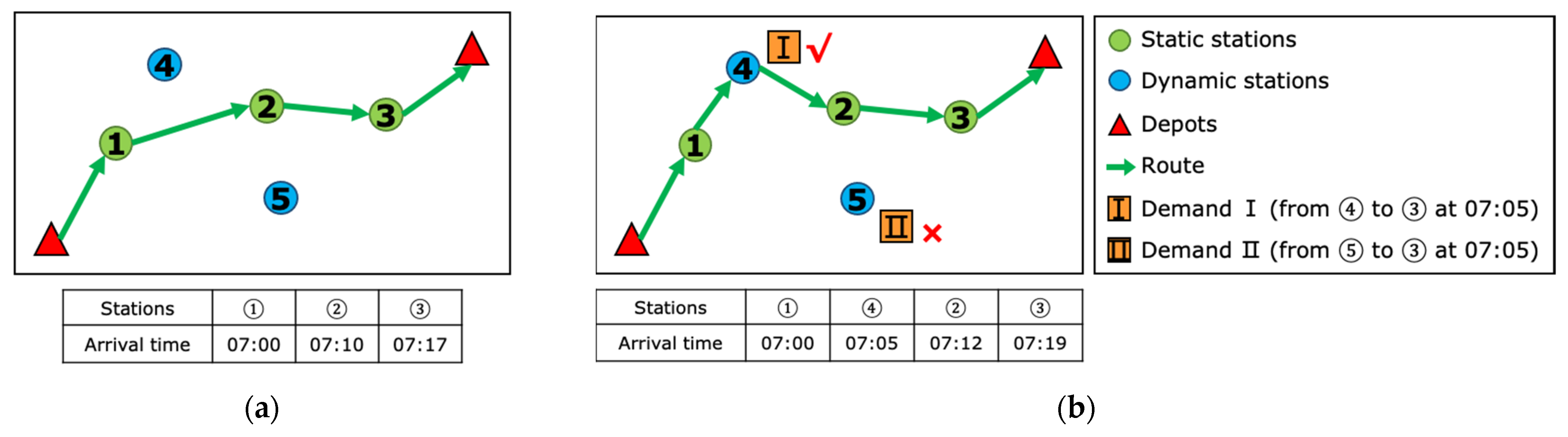
Under such circumstances, flex-route transit is expected to bring a feasible way to provide specific services for stable demands and unstable demands, respectively [6,17,18,19]. In flex-route transit, stable demands enjoy fixed service, while unstable demands receive flexible service. Considering the spatial similarity among stable demands, we define the stations related to stable demands as static stations, and other nonstatic stations as dynamic stations. Correspondingly, stable demands and unstable demands can be also named static-station-based demands and dynamic-station-related demands, respectively. It is ruled that static-station-based demands could be fixedly served by flex-route transit without submission. However, dynamic-station-related demands must be submitted, and these passengers wait for acceptance or rejection. As shown in Figure 1, the bus visits static stations (marked as green circles) in all cases. In the case that no dynamic-station-related demand appears or all these demands are rejected, the route only consists of static stations, as Figure 1a shows, which can be named base route. In another case with dynamic-station-related demands submitted, the problem is whether to serve demands and when to visit dynamic stations. As Figure 1b shows, Demand Ⅰ is accepted with the related dynamic station ④ (marked as a blue circle) visited at 07:05, while Demand Ⅱ is rejected. This is because deviating to dynamic station ⑤ (the origin of Demand Ⅱ) would spend much time, resulting in unacceptable waiting time and increasing cost. Attracted by the characteristics of flex-route transit, both academia and industry have shown great interest. In the early years, scholars [20,21,22,23] provided fixed service and dial-a-ride service for common passengers and special demands, respectively. Later, many studies [24,25,26,27,28,29,30,31,32] designed flex-route transit to serve static-station-based demands and dynamic-station-related demands. And bus operators successfully applied it in rural areas in the USA [33].
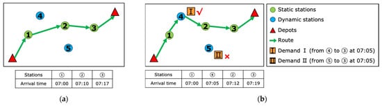
Figure 1.
The types of routes in flex-route transit. The description of each panel is as follows: (a) base route; (b) the route with dynamic stations visited.
For the optimal transportation service, station design and route planning are two important steps. Of note, the design framework of flex-route transit is different from other kinds of transits.
In terms of station design, traditional transit seeks the optimal station location or spacing with the objects of minimum total cost and maximum demand coverage [34,35,36,37,38], while the stations in customized transit and demand-responsive transit are mainly decided by demands [7,13,16,39,40,41,42]. Differently, Flex-route Transit needs to distinguish static stations beforehand, for serving stable demands fixedly. Most of the relevant studies [24,25,26,27,28,29,30,31,32] relied on a single feature, and we consider their methods as different variants of the single-feature classification method. For example, Qiu et al. [24] calculated the passenger flow of each station and manually chose the large-flow stations as static stations. But manual selection may miss some static stations due to the disadvantages of individual experiences. Instead of manual selection, Sun and Liu [30] input the spatial position of each station into the k-means clustering algorithm to divide k clusters, of which the centers served as static stations. However, these single-feature classification methods may fail to capture the comprehensive characteristics of stations. For example, facing the stations with certain stable demands but few passengers in total, one may mistake these stations for dynamic stations due to the one-sided judgment of total flow.
In terms of route planning, traditional transit runs along the shortest routes with all stations visited [36,37,38]. Similarly, the base routes in flex-route transit are planned with all static stations visited. Most scholars [24,25,26,27,28,29,30] only set one shortest route, while Qiu et al. [31] generated two base routes for round-trip demands. Furthermore, Han and Fu [32] proposed a multi-route planning model with consideration of high-frequency and multi-direction demands, but these base routes suffered from route-length problems. Different from the fixed service for all stations in traditional transit, flex-route transit can provide flexible service for unstable demands at dynamic stations. Thus, most studies planned base routes first, and then inserted dynamic stations into base routes according to demands. The above method can be called the base-route-predesigned planning method. According to the input demands, the route plan can be divided into two types. The offline plan only focuses on reserved demands, while the online plan is generated based on real-time demands. Considering the type of the generated plan, existing studies related to flex-route transit can be divided into three groups. The first group of studies [24,25,26,27,30,31] considered the reserved-demand service problem as the vehicle routing problem and solved it with an offline plan generated in advance, similar to the offline routes planning of customized transit [13,16,39,40,41]. But they both ignored real-time demands during the bus operation. In contrast, without preparing an offline plan, the second group (e.g., Liu et al. [28], Han and Fu [32]) considered the real-time-demand service problem as the station insertion problem and found the optimal insertion of dynamic stations, similar to the online routes planning of demand-responsive transit [42]. With consideration of the offline and online routes planning, the third group, such as Zheng et al. [29], generated an offline plan first, and then updated it into an online plan. Overall, the base-route predesigned planning method would fix the number of base routes and the sequence of static stations in advance, which may have a bad influence on the acceptance rate of dynamic-station-related demands. To avoid the above disadvantages, we propose the two-stage planning method to provide service for both reserved demands and real-time demands, without predesigning base routes.
Aiming to improve the service of flex-route transit, this paper proposes a framework for designing flex-route transit based on multi-type demands. To overcome the disadvantages of manual selection based on a single feature, the multi-feature-based classification method is presented to classify static stations and dynamic stations through hierarchical clustering algorithm based on multiple kinds of historical features. And, to break the limit of predesigned base routes, two-stage planning method is designed to obtain a multi-route plan with the flexible combination of demands and regular travel patterns through multi-route design model and route modification model. For convenience, the abbreviated form of some words in this paper are shown in Table 1.

Table 1.
Abbreviations.
The main contributions of this study can be summarized as follows:
- (1)
- Compared with the single-feature classification method, this paper proposes MFCM to evaluate multiple kinds of station features, which performs better in recognizing the differences between stations.
- (2)
- Instead of predesigning base routes, we generate a multi-route plan by flexibly integrating reserved demands and regular travel patterns. TSPM can serve 20% more demands with less traveling time per passenger than the base-route predesigned planning method.
- (3)
- Numerical experiments prove the applicability of FT and show that, compared with traditional transit, our proposed FT transports demands more effectively and saves nearly 40% of the total cost.
The remainder of this paper is organized as follows. Section 2 proposes the FT design framework. Section 3 describes MRDM and RDGA. Section 4 introduces RMM and greedy algorithm. Section 5 analyzes the advantages of the proposed methods and FT based on realistic demands, and tests the adaptability of FT in generated cases. Section 6 concludes the paper and discusses future work.
2. Multi-Type Demands Oriented Framework
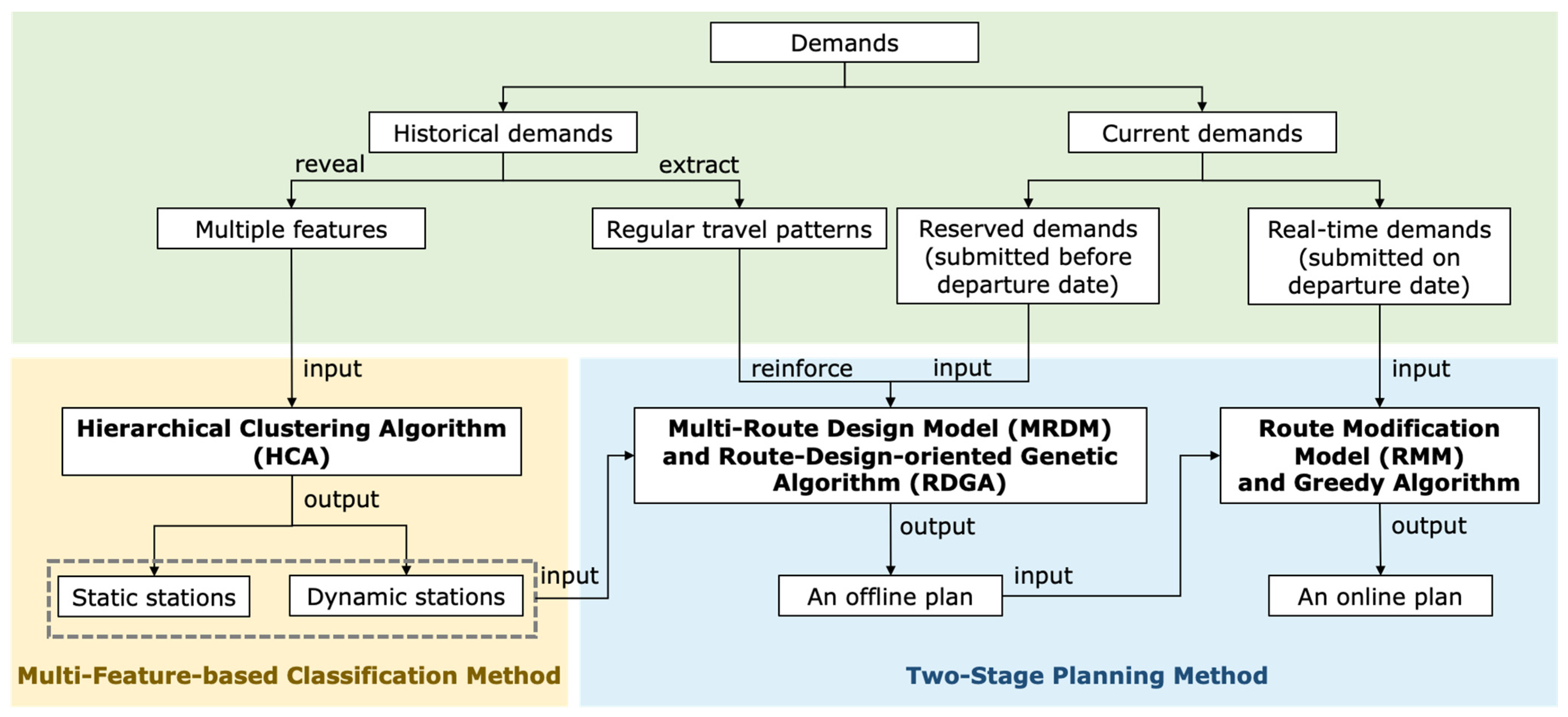
In our proposed framework, as shown in Figure 2, there are three important parts, including multi-type demands, multi-feature-based classification method (MFCM), and two-stage planning method (TSPM).
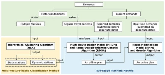
Figure 2.
The design framework based on multi-type demands.
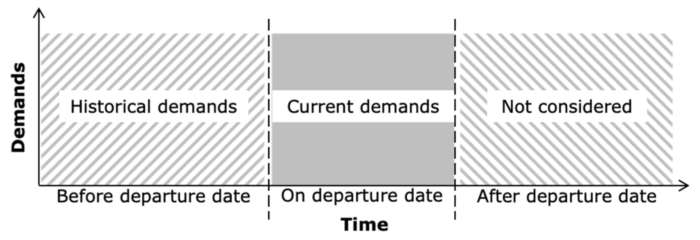
As the green part reflects, demands need to be classified into specific types beforehand. In the beginning, we make the first division according to the departure time of demands, as shown in Figure 3. If we assume that the departure date of the FT route plan is , historical demands refer to the passengers who have set off before the departure date, such as , and current demands are those who will depart on .

Figure 3.
The types of demands.
Based on historical demands, we obtain multiple kinds of station features and input these features into MFCM to solve the classification problem. In addition, we extract regular travel patterns from historical demands, which can reinforce the service capacity for static-station-based demands. In this paper, a travel pattern shows that a passenger frequently travels along with the same OD during a similar time, and the regularity reflects that a large number of passengers share a spatially and temporally similar pattern. For example, a passenger and his/her colleagues start from adjacent origin stations to the same workplace in the morning peak on weekdays. According to the definition, this travel pattern of the above OD in the morning peak can be considered as a regular travel pattern.
In terms of current demands, we make the second division according to the submission time, since dynamic-station-related demands must be submitted to FT. Thus, the submitted current demands are further divided into reserved demands and real-time demands. Reserved demands have been submitted before the departure date, such as , while real-time demands will be submitted on the departure date.
As the yellow part reflects, with the input of station features, MFCM can recognize static stations and dynamic stations through HCA, which will be discussed in Section 2.1.
As the blue part reflects, with the input of classified stations, regular travel patterns, and demands, TSPM can generate the FT route plan through two stages, which can be learned from Section 2.2.
2.1. Multi-Feature-Based Classification Method (MFCM)
As to station classification, MFCM is presented with the use of multiple features and HCA. Compared with the single-feature classification methods proposed by existing studies, MFCM captures comprehensive features of each station and introduces a data-driven algorithm to solve the classification problem.
Firstly, three kinds of features are chosen, including passenger flow, related-OD-pair amount, and loyal-passenger flow. Among these features, the passenger flow can evaluate the service level of a station. And the related-OD-pair amount records the OD pairs, of which the origin or destination is the target station, reflecting the service range of a station. In addition, the loyal-passenger flow refers to the number of passengers who frequently travel along with the same OD at a certain time, which embodies the service stability of a station. With the consideration of these features, the performance of each station can be evaluated more comprehensively. And station features need to be standardized according to the following formulation, , where represents the standardized feature, represents the original feature, and refer to the average value and standard deviation of all stations, respectively.
Then, HCA [43,44] is adopted to divide two clusters based on the standardized features above. The division includes three steps as follows. (1) Initialize each station as an independent cluster. (2) Calculate the average distance between two clusters and merge the nearest clusters into a new cluster. (3) Repeat Step (2) until only two clusters are left. In Step (2), the average distance refers to the average value of the weighted Euclidean distance from stations in one cluster to stations in another. And the weighted Euclidean distance is formulated as follows: . represents the weighted Euclidean distance between two stations, belong to the set of stations, represents each feature, and refers to the weight coefficient of each feature.
Finally, static stations and dynamic stations are distinguished by comparing the average features of the last two clusters. The cluster with larger values of features can be considered as the set of static stations, because a static station attracts many passengers, such as loyal passengers, and shares strong relationships with other stations.
2.2. Two-Stage Planning Method (TSPM)
As to route planning, TSPM is designed based on classified stations and submitted demands. Firstly, we propose MRDM to generate an offline plan based on reserved demands and regular travel patterns. Secondly, we use RMM to optimize an online plan by inserting the related dynamic stations based on the offline plan and real-time demands. MRDM, RMM, and their solutions are further introduced in Section 3 and Section 4.
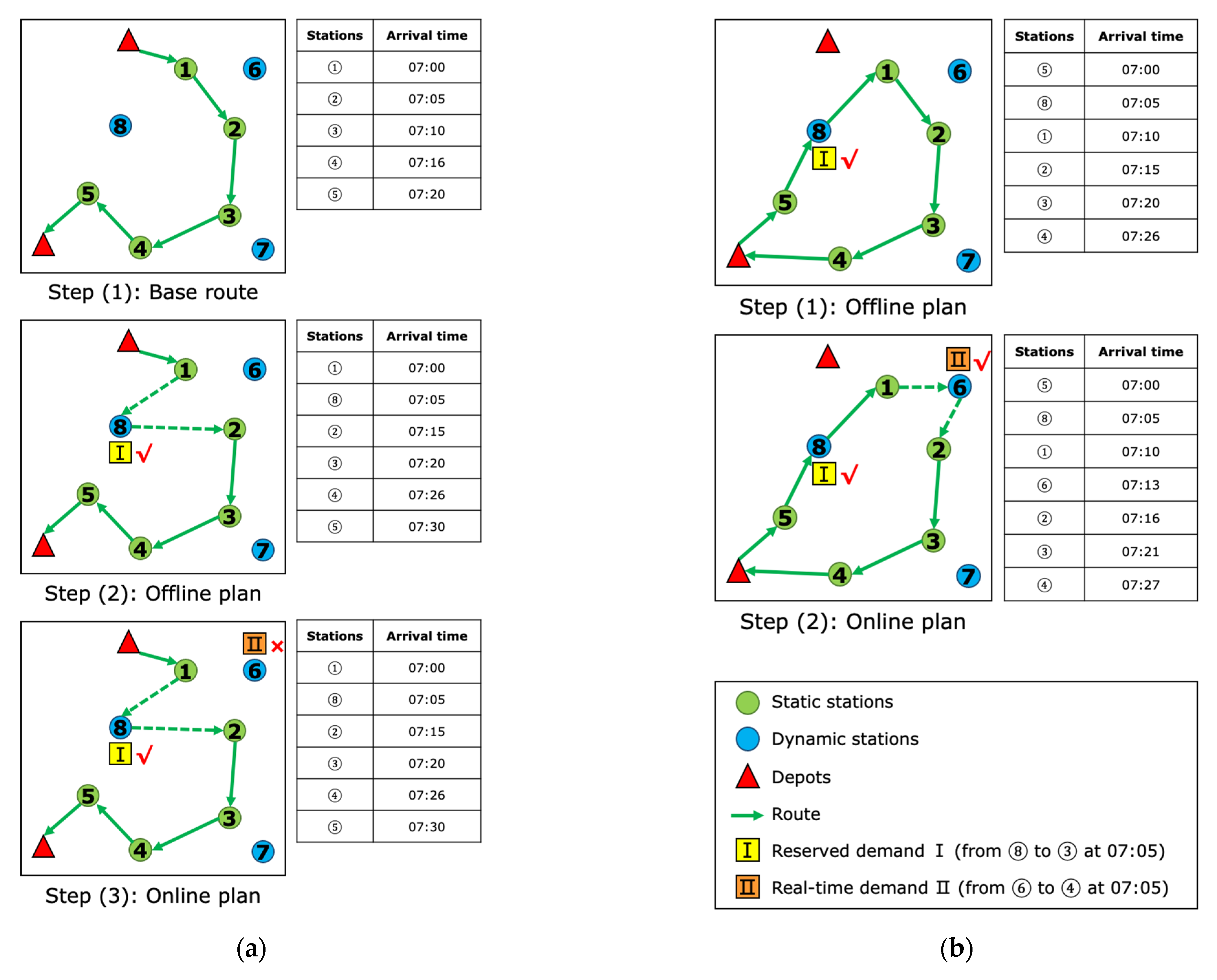
Compared with the base-route predesigned planning method used by previous studies, TSPM does not need to predesign base routes and optimizes the offline routes planning by flexibly integrating reserved demands and regular travel patterns. To explain the difference between TSPM and the base-route predesigned planning method, we conduct a comparison based on a small network and generated demands. As Figure 4 illustrates, there are five static stations, three dynamic stations, and two demands.
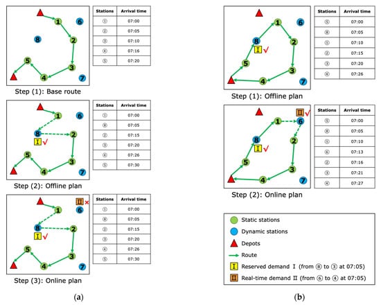
Figure 4.
A comparison between two planning methods. The description of each panel is as follows: (a) the process of the base-route-predesigned planning method; (b) the process of TSPM.
The base-route predesigned planning method generates the FT online plan through three steps, as shown in Figure 4a:
- (1)
- Regardless of current demands, a base route is designed to visit all static stations with minimum distance.
- (2)
- Next, focusing on reserved demands, the bus can serve Demand Ⅰ since the constraints of passenger waiting time and bus single-trip time are both satisfied. An offline plan is generated by inserting dynamic station ⑧ into the base route.
- (3)
- Then, considering real-time demands, Demand Ⅱ is rejected for the reason that deviating to dynamic station ⑥ would exceed the maximum waiting time of Demand Ⅱ. Thus, the online plan remains the same as the offline plan with 30 minutes of the bus single-trip time.
Differently, TSPM obtains an online plan through two steps, as Figure 4b shows:
- (1)
- With the flexible combination of reserved demands and regular travel patterns, Demand Ⅰ is served. And the offline plan visits all static stations and dynamic station ⑧ within an acceptable distance.
- (2)
- Then, considering real-time demands, the online plan accepts Demand Ⅱ with the acceptable waiting time and little deviation to dynamic station ⑥, with 27 minutes of the bus single-trip time.
3. Multi-Route Design Model (MRDM) and Its Solution
3.1. Model Assumptions
For the optimal plan, MRDM is constructed based on the following assumptions:
- (1)
- The volume of a bus is fixed.
- (2)
- The number of available buses is unlimited.
- (3)
- The bus dispatch is not considered.
- (4)
- The bus ticket is free.
- (5)
- The driving time between two stations is known beforehand and set as the minimum value according to the shortest path.
- (6)
- The travel plans of reserved demands and real-time demands are known, including the origin station, the destination, and the demand time.
- (7)
- The bus arrival time at a station is equal to the boarding time of accepted passengers whose origin is the same station.
3.2. Model Formulation
In route planning, the related notations are summarized in Table 2.
Table 2.
Notations.
According to the notations above, MRDM is formulated as follows. The constraints in MRDM mainly focus on trips, since a plan consists of many trips. Of note, some constraints in MRDM are different from the traditional multi-route planning model. For example, FT should satisfy all static stations, as Equation (12) shows.
- Objective function:
In MRDM, the objective function (1) seeks the optimal balance among three aspects, including the bus running cost, the passenger waiting time loss, and the rejection loss. As function (1) shows, the bus running cost relies on the sum of single-trip time. And the passenger waiting time loss is targeted at the accepted reserved demands, while the rejection loss is decided by the rejected reserved demands.
- Trip constraints:
Constraints (2) to (7) determine the station sequence of each trip. Constraints (2) and (3) aim to avoid turning around in practical operation. Constraints (4) and (5) give the bound of the trip’s arrival time at visited stations and depots, while constraints (6) and (7) set the bound of the single-trip time.
- Demand constraints:
Constraints (8) to (11) build the temporal and spatial relationship between trips and accepted demands. Constraint (8) requires the trip to match the OD of the accepted demand. Constraints (9) and (10) limit the trip’s arrival time at the corresponding origin station. In addition, constraint (11) restricts that each demand can be served, at most once.
- FT service constraints:
Constraints (12) and (13) ensure fixed service for static stations and regular patterns.
- Decision variables:
3.3. Model Solution
MRDM aims to solve the multi-route planning problem that is regarded as an NP-hard problem [45,46]. Especially confronting spatially and temporally varying demands, the solution scale increases sharply, and the computational time may be unacceptable. Thus, we design the route-design-oriented genetic algorithm (RDGA) to improve MRDM.
RDGA is similar to the traditional genetic algorithm, as Algorithm 1 shows.
| Algorithm 1. Route-design-oriented genetic algorithm |
Input: the population size , the maximum iterations , and others |
|
Output: the global best value and the global best individual |
In the beginning, initialize and encode several offline plans to generate the initial population. Then, conduct optimization to generate offspring individuals and evaluate them to choose the best individual with the minimum cost. If the termination condition is not reached, it will repeat the individual optimization and evaluation. Otherwise, it will end and output the best individual that is decoded into the best plan.
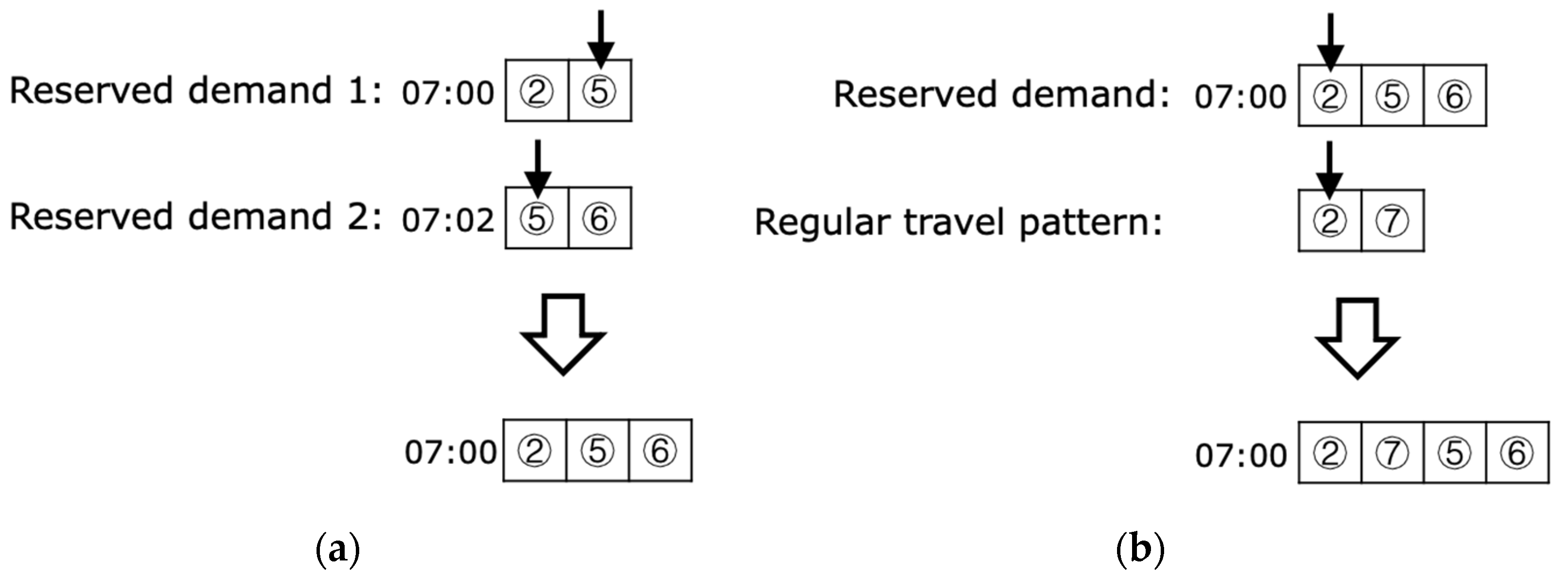
- Population initialization.
We initialize a population through plan initialization and individual encoding.
In plan initialization, we firstly integrate several reserved demands according to the station similarity and the demand-time similarity, as shown in Figure 5a. Secondly, regular travel patterns are combined with reserved demands according to the station similarity, as shown in Figure 5b. Thirdly, we match each trip with the nearest depots.
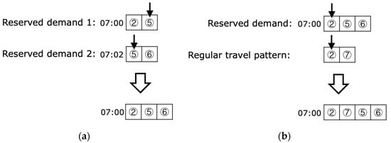
Figure 5.
The key steps in plan initialization. The description of each panel is as follows: (a) the example of combining two reserved demands; (b) the example of combining a reserved demand and a regular pattern.
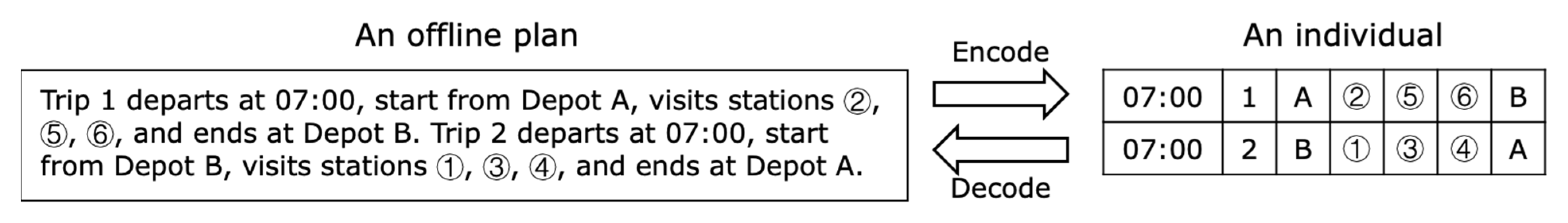
In individual encoding, we set the encoding rules that each trip in a plan represents a line in an individual, and each line consists of the trip’s departure time, the number, and the station sequence, as shown in Figure 6.
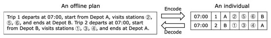
Figure 6.
The example of individual encoding and decoding.
Finally, we repeat the plan initialization and individual encoding until the number of generated individuals reaches the population size .
- Individual evaluation and optimization.
We evaluate each individual according to the objective function (1) of MRDM. A better individual refers to a plan with a smaller objective value.
Then, individuals are optimized through selection, crossover, and mutation. In terms of selection, we adopt the tournament mechanism by randomly selecting two individuals, and retain the better one with a smaller objective value. The above step is repeated until the number of remaining individuals reaches the population size . In terms of crossover, according to the crossover probability , we randomly swap the segments (from the same static station to the next visited station) between two individuals, as shown in Figure 7a. In terms of mutation, according to the mutation probability , we randomly delete one element (a dynamic station) of an individual, as shown in Figure 7b.
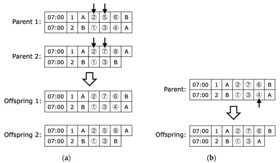
Figure 7.
The key steps in individual optimization. The description of each panel is as follows: (a) the example of individual crossover; (b) the example of individual mutation.
- Iteration termination.
Once either of the termination conditions is reached, we end the iterations and output the best individual. One termination condition is to judge whether the number of iterations reaches the maximum value , as shown in Algorithm 1. The other is to judge whether the difference between the best individuals of the last two iterations is less than the threshold , as shown in Algorithm 2.
- Individual decoding.
We decode the best individual, as shown in Figure 6. According to the decoding rules, each line in an individual represents a trip in a plan, and the first element, second element, and other elements of a line refer to the trip’s departure time, the number, and the station sequence, respectively. For example, an individual with two lines can be decoded into a plan with two trips. Trip 1 departs at 07:00, starts from Depot A, visits stations ②, ⑤, and ⑥ in order, and ends at Depot B, while Trip 2 departs at 07:00, starts from Depot B, visits stations ①, ③, and ④ in order, and ends at Depot A.
Algorithm 2. Termination judgement |
Input: , the threshold and others |
|
Output: the global best value , the global best individual , and |
4. Route Modification Model (RMM) and Its Solution
4.1. Model Formulation
According to the notations (summarized in Table 2) and the assumptions (listed in Section 3.1), RMM is formulated as follows. Different from MRDM, RMM does not set fixed-service constraints (12) and (13) because each online trip must retain the station sequence of the corresponding offline trip.
- Objective function:
In RMM, the objective function (17) aims to minimize the real-time cost, where refers to the acceptance or rejection of a real-time demand , calculated by , and represents the single-trip time of trip after serving demand , calculated by . If a real-time demand is accepted (), the real-time cost consists of the bus detour cost and the passenger waiting time loss. Otherwise, it refers to the rejection loss. As the first part of function (17) shows, the bus detour cost focuses on the single-trip time difference caused by accepting the real-time demand .
- Constraints:
If the trip accepts the real-time demand (), it must meet the requirement of station sequence, as constraints (2) to (7) show, maintain the service for reserved demands, as constraints (8) to (10) show, and build the temporal and spatial relationship with the real-time demand , as constraints (18) to (21) show.
If trip rejects demand (), it does not change.
- Decision variables:
4.2. Model Solution
RMM aims to solve the station insertion problem for each real-time demand. When generating an online plan, we adopt greedy algorithm, as Algorithm 3 shows. The solution process can be described as follows:
- (1)
- Input the first-received real-time demand and the offline plan into RMM;
- (2)
- Start greedy algorithm and initialize an online plan;
- (3)
- Search for candidate trips, of which the operational time meets the demand time;
- (4)
- Insert the related dynamic stations of the demand into each candidate trip based on the spatial and temporal similarity, and generate the adjusted plans;
- (5)
- Evaluate the adjusted plans and the online plan according to Equation (17);
- (6)
- Output the online plan with minimum cost and end greedy algorithm;
- (7)
- Input the next real-time demand and the online plan into RMM and repeat steps (2) to (6) until FT responds to all received real-time demands.
| Algorithm 3. Greedy algorithm |
Input: a real-time demand , the offline plan , the online plan , the rejection loss , and others |
|
Output: the online plan and the minimum cost |
5. Result Analysis
5.1. Experiment Preparation
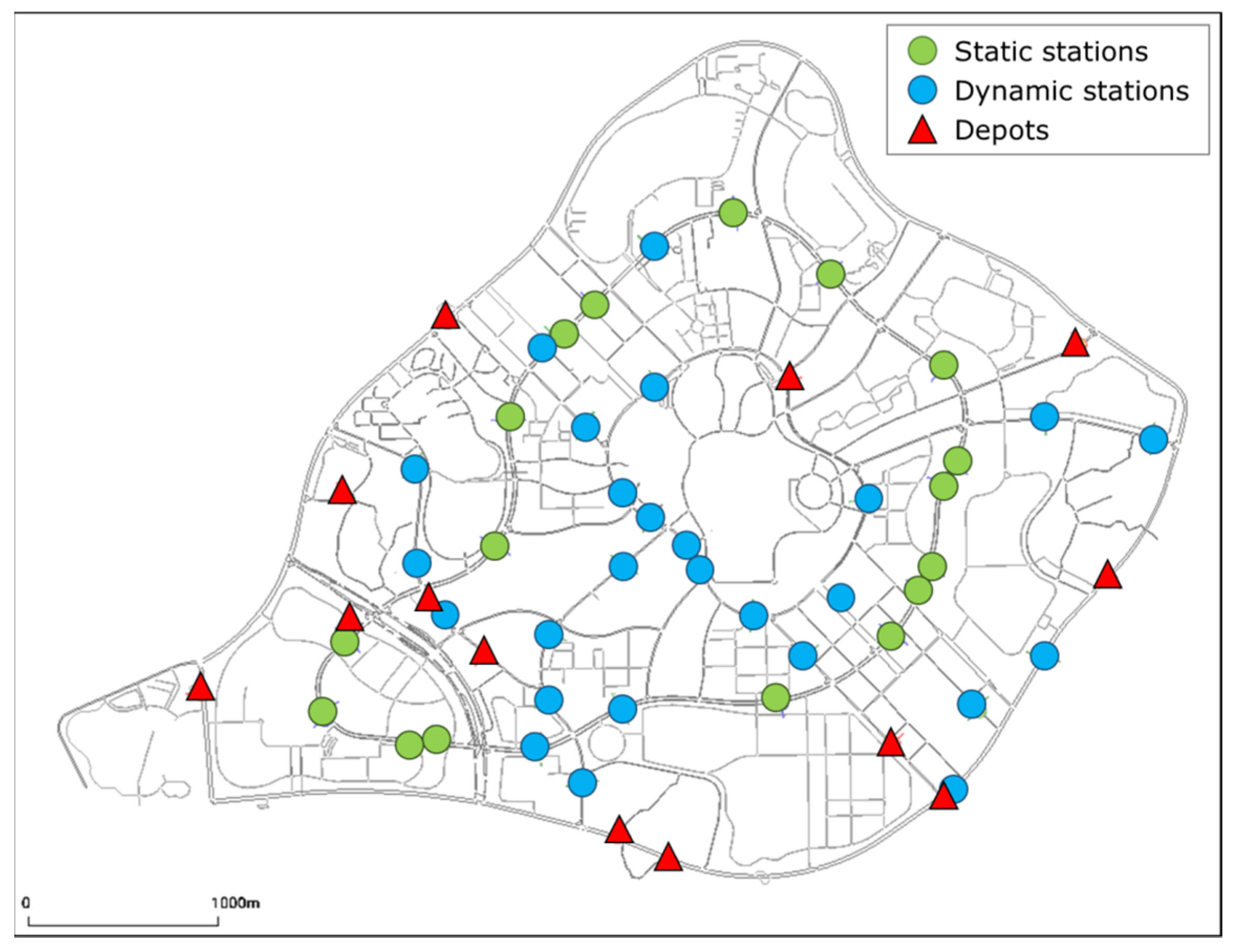
In this study, Guangzhou Higher Education Mega Center in China is set as the research area, in which 70 bus stations and 13 depots are situated, as Figure 8 shows. In the research area, traditional public transit can cover all bus stations and transport most passengers from one station to another. Among these traditional routes, we choose the five routes with large passenger flow as the traditional transit (TT) route plan.
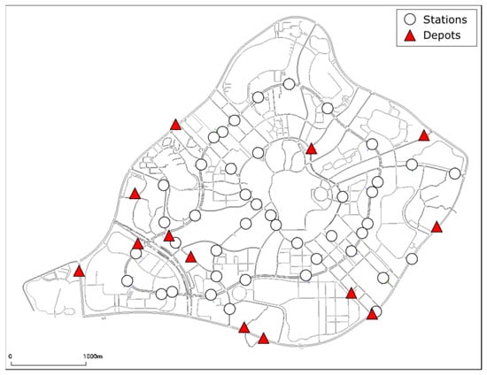
Figure 8.
Research area.
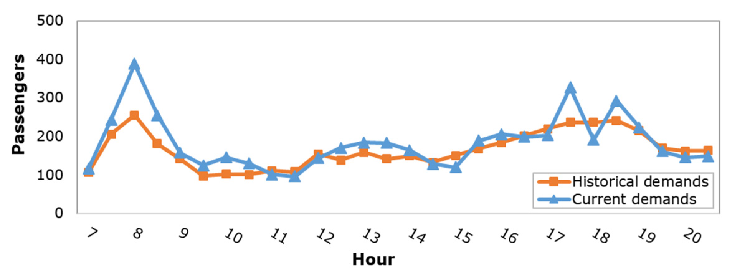
For data preparation, we collect the information related to TT, including the smart card data and the bus driving time between stations. Based on the smart card data above, we obtain the realistic demands of passengers who travelled in the research area from 07:00:00 to 21:00:00. And the demands are divided into current demands (happening on 26 September 2017) and historical demands (happening from 18 to 24 September 2017). The above demands are shown in Figure 9, where the black line reflects the daily average value of historical demands. In terms of the passenger flow, there are over 100 passengers per hour in the research area. Of note, TT served nearly 400 passengers in the morning peak hour on 26 September. It illustrates that our research area is a larger network with numerous demands, compared to the small network (with less than 90 demands per hour) used in previous studies. In terms of the temporal characteristics, both kinds of demands have similar distribution during the operational time, which reveals that the performance of stations on 26 September is similar to the historical performance.
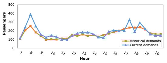
Figure 9.
Historical demands and current demands.
Thus, we use historical demands for station classification and regular pattern mining, and input current demands into route planning and evaluation. For route planning, dynamic-station-related demands are selected from current demands and further divided into reserved demands (accounting for 80%) and real-time demands (accounting for 20%).
For FT design, some parameters are set as fixed values, as Table 3 summarizes. We assume that the economic condition of the research area is similar to the one in previous studies [26,29,31], and set the two parameters to be USD 1.00/min and USD 0.25/min. Of note, we consider different punishment of demand rejection under the offline and online route planning. To evaluate an offline plan, the unit rejection loss is defined to be the product of the average travel time and the unit time loss of a passenger, calculated as . For the evaluation of an online plan, we set the unit rejection loss twice as large as , since the rejected real-time demands have suffered waiting time loss at their origin stations. Considering the actual operation of TT in the research area, parameters , the bus volume, and the trip’s departure-time interval are 1 min, 30 min, 50 min, 60 passengers, and 10 min, respectively. And the maximum waiting time of each passenger is equal to the trip’s departure-time interval. In addition, we set the RDGA-related parameters according to Han [32].
Table 3.
Notations setting.
Based on the above parameters, simulation experiments are developed in Spyder 5.1.5 software on the computer (with i5-8259U CPU, Windows 10 system).
For service evaluation, we set several indices, as described in Table 4. The first three indices are used to analyze the service capacity of a plan, while the fourth to seventh indices are set for cost-efficiency evaluation. Especially in total cost, the rejection loss of rejected reserved demands is calculated with the use of , while the rejection loss of rejected static-station-based demands and rejected real-time demands uses . In addition, average waiting or on-bus time per passenger can reflect the passenger experience under a plan. Moreover, we calculate the difference of two plans in rate or value for comparison.
Table 4.
Evaluation indices description.
5.2. Sensitivity Analysis
In MFCM, represent the weight coefficient of station features, which plays an important role in calculating the weighted Euclidean distance between two stations.
To analyze the impact of on station classification, different values of are used to simulate the various results of MFCM, under the premise of keeping other parameters the same and the constraint of “”. Figure 10a shows the ratio of the average passenger flow of static stations to dynamic stations during each time period, while Figure 10b reflects the ratio of the average related-OD-pair amount. The ratio of the average loyal-passenger flow is not considered, since there may be no loyal passenger getting on or off at dynamic stations. A larger ratio refers to the better recognition of differences between static stations and dynamic stations. When the value of or is increasing, the two ratios are improved. Especially when , MFCM reaches the best results, which means that MFCM can distinguish static stations well, with a relatively larger weight coefficient of the passenger flow. However, it is not recommended to rely on the single feature (e.g., the passenger flow) to classify stations, as Section 5.4 describes.
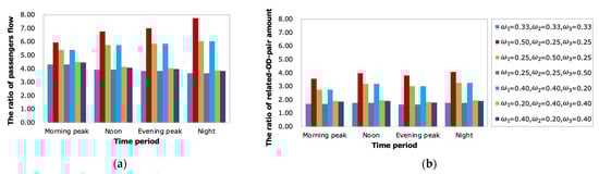
Figure 10.
Station-feature comparisons under different values of . The description of each panel is as follows: (a) the ratio of passenger flow; (b) the ratio of related-OD-pair amount.
After analysis, we set parameters to be 0.50, 0.25, and 0.25, respectively.
5.3. Application Analysis
To analyze the feasibility of the proposed FT, we apply the FT design framework in the research area based on realistic demands. In addition, the bus stations in the research area are defined as candidate stations to be classified and visited.
Firstly, MFCM is applied to divide candidate stations into two clusters based on historical demands. The temporal characteristics of the above clusters are summarized in Table 5. The stations in Cluster 1 serve 26 passengers and visit nearly 20 pairs of OD on average. Especially in the peak hours, there are several loyal passengers starting from or ending at these stations. As to all listed features in Table 5, these stations perform better than those in Cluster 2. This means that the stations in Cluster 1 attract more passengers, including loyal ones, and have stronger relationships with other stations. Therefore, we consider stations in Cluster 1 as static stations, and define the other stations as dynamic stations.
Table 5.
Station features under SCM.
According to the above classification, Figure 11 shows the actual position of static stations and dynamic stations in the research area. There are 26 static stations, 44 dynamic stations, and 13 bus depots. Of note, static stations are all situated in the middle loop, which shows that stable demands usually travel along the middle loop in the research area. Meanwhile, dynamic stations are mainly situated in the inner loop or radial roads, which reflects the spatial variations in dynamic-station-related demands.

Figure 11.
The position of static stations, dynamic stations, and depots.
Secondly, TSPM is applied to generate the FT plan based on classified stations and current demands. Through MRDM and RDGA, we design an offline plan for reserved demands. As Figure 12 illustrates, with the help of RDGA, the objective value of MRDM drops from USD 16,800 to USD 14,280 and reaches the minimum within 130 iterations. Then, through RMM and greedy algorithm, we obtain an online plan based on the offline plan and real-time demands.
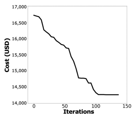
Figure 12.
The performance of RDGA.
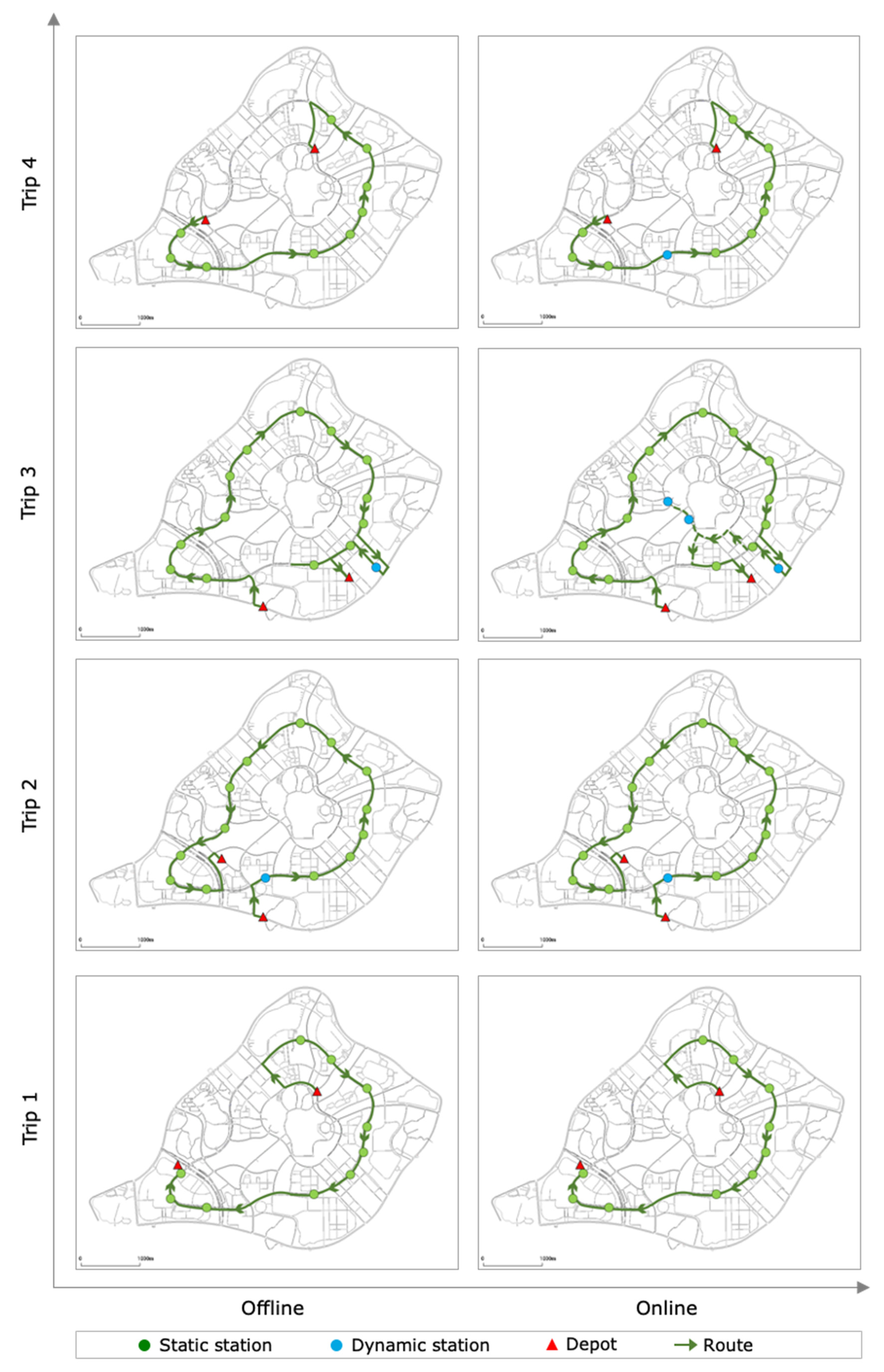
Some trips of the above offline plan and online plan are shown in Figure 13, respectively. With consideration of regular travel patterns, trips visit static stations in different orders and mainly run along the middle loop, such as Offline Trip 1 and 3. Of note, Offline Trip 3 visits dynamic stations with acceptable detours. In addition, each online trip retains the station sequence of the corresponding offline trip and serves the accepted reserved demands, such as Online Trip 3. Overall, static stations are visited fixedly in FT, while reserved demands and real-time demands receive flexible service under specific constraints.
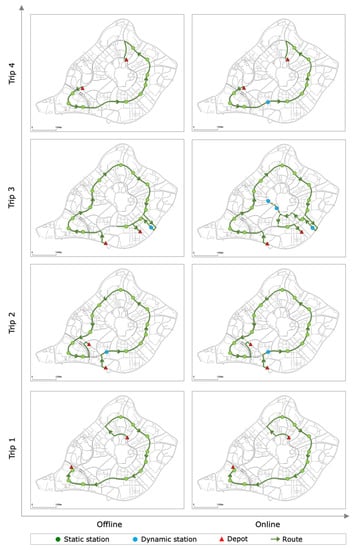
Figure 13.
The offline trips and online trips departing at 16:00.
Furthermore, we make a comparison between the performance of TT and FT based on the research area and realistic demands, as Table 6 shows. In terms of service capacity, the stations effective-utilization rate of FT reaches 100%, while that of TT is lower than 70%. This is because TT provides fixed service for all stations, including no-demand stations, resulting in empty-loaded cases and unnecessary gas emissions. In addition, the demands acceptance rate of FT has reached 91%, though it is a bit less than that of TT. In terms of cost efficiency, each trip under FT serves seven more passengers than the trip under TT. And FT saves nearly 40% of total cost and spends less on each passenger compared with TT. This demonstrates that the flexible service of FT on little-demand stations (as well as dynamic stations) can satisfy certain demands with minimum cost, which can transport demands more effectively and alleviate environmental pollution to a large extent.
Table 6.
Route-performance comparisons between TT and FT.
We conclude that it is feasible to apply FT in the research area, which can promote service flexibility, cost efficiency, and social sustainability compared with TT.
5.4. Method Comparison
To analyze the advantages of this study, we compare our proposed methods with those methods in previous studies based on the research area and realistic demands.
Considering station classification, we conduct an experiment to compare MFCM and the single-feature classification method, since most studies [24,25,26,27,28,29,30,31,32] relied on a single feature to classify stations. In this experiment, the single-feature classification method refers to ranking stations in descending order based on passenger flow, and then choosing the top 20% as static stations.
The above comparison results based on historical demands are shown in Table 7. Each value in the table represents a ratio of the average passenger flow of static stations to dynamic stations. A larger ratio refers to the better recognition of differences between static stations and dynamic stations. During the operational time, the results of MFCM are better than the result of the single-feature classification method. Of note, MFCM performs best at night, and the difference between the two methods is over 3.5 times.
Table 7.
Station-feature comparisons between two classification methods.
Considering route planning, we make a comparison between TSPM and the base-route-predesign planning method (called three-step method in this section). And both methods have considered reserved demands and real-time demands. The three-step method consists of the multi-base-route design model proposed by Han and Fu [32] and the offline and online station-insertion models proposed by Zheng et al. [29].
Table 8 summarizes the comparison results of two planning methods based on the same classified stations under MFCM. In terms of service capacity, TSPM matches 6% more OD pairs and accepts 5% more demands than the three-step method. It verifies that the integration of reserved demands and regular travel patterns can make a better arrangement of dynamic stations, and further increase the number of accepted demands. In terms of passenger experience, both reserved demands and real-time demands enjoy a faster service under TSPM, with less waiting time and on-bus time than the result under the three-step method. This is because TSPM can respond to demands at a higher speed and serve dynamic stations with fewer detours, without limitation of the number or station sequence of base routes.
Table 8.
Route-performance comparisons between two planning methods.
In general, our proposed methods outperform other methods in the above experiments. Of note, MFCM performs better in differences recognition than the single-feature classification method. And TSPM offers service with more flexibility and better quality than the base-route predesigned planning method.
5.5. Adaptability Analysis
Considering that current demands may change a lot on different dates, we test the adaptability of FT on a set of cases with different dynamic-station-related demands. In each generated case, the ratio of dynamic-station-related demands to all current demands (denoted as ψ) is chosen from the range [0, 100%]. For example, means that only 10% of current demands start from or end at dynamic stations, while the other demands travel between static stations. In addition, the number of all current demands and the ratio of reserved demands to all dynamic-station-related demands remain at 3000 and 80%, respectively.
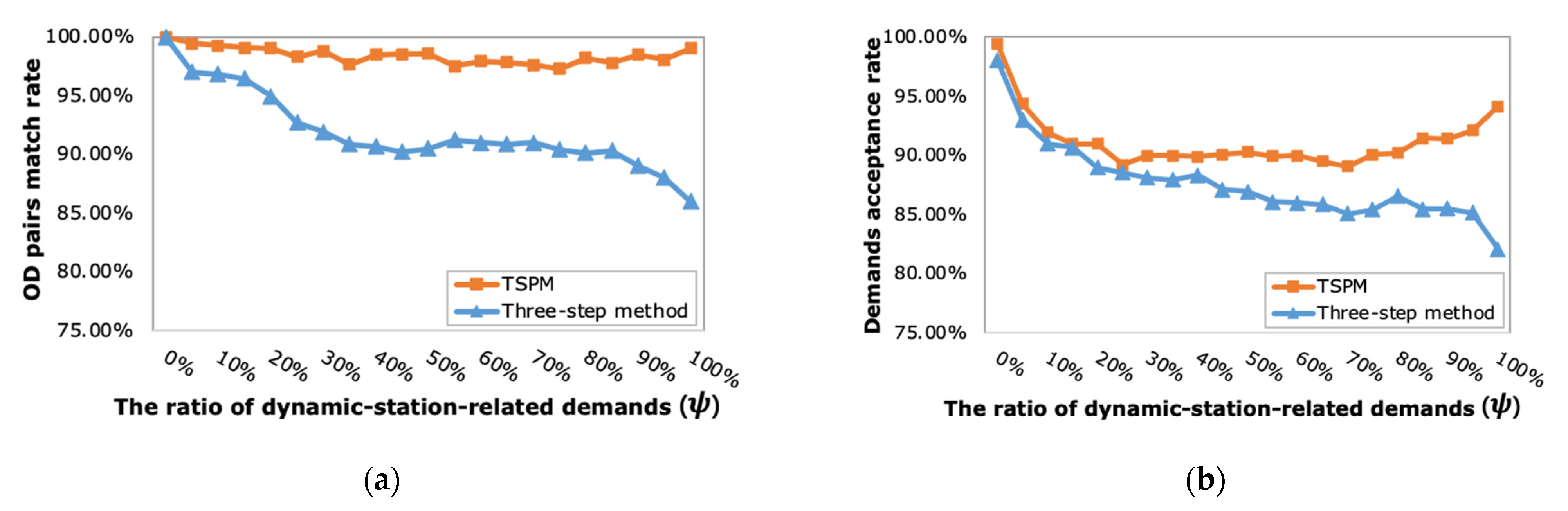
In the cases with different values of , we conduct an experiment to compare TSPM and the base-route-predesign planning method (the three-step method described in Section 5.4). Figure 14 shows the comparison results of two planning methods based on the classified results under MFCM. When , it refers to the special case that all passengers travel between static stations. In this case, FT can match all demand-related OD pairs and serve most of the static-station-based demands under each method. When increases from 0 to 60%, the rate differences between the two methods become larger. Especially when , TSPM helps FT to match 10% more OD pairs and to serve 5% more demands than the three-step method. This is because the integration of reserved demands and regular travel patterns in TSPM can break the limit of predesigned base routes, and thus make a better arrangement of dynamic stations. When increases from 60% to 100%, TSPM promotes two rates slightly but the rates keep dropping under the three-step method. It demonstrates that TSPM adapts well to dynamic-station-related demands with full consideration of reserved demands in the first stage.

Figure 14.
Route performances in the generated cases with different values of . The description of each panel is as follows: (a) OD pairs match rate; (b) demands acceptance rate.
Moreover, given that dynamic-station-related demands may be submitted on different dates due to individual preference, the adaptability of FT is further tested on a set of cases with different reserved demands and real-time demands. In each generated case, the number of all current demands remains at 3000. And the ratio of dynamic-station-related demands to all current demands () is chosen from the three values (), while the ratio of reserved demands to all dynamic-station-related demands (denoted as ) is chosen from the range .
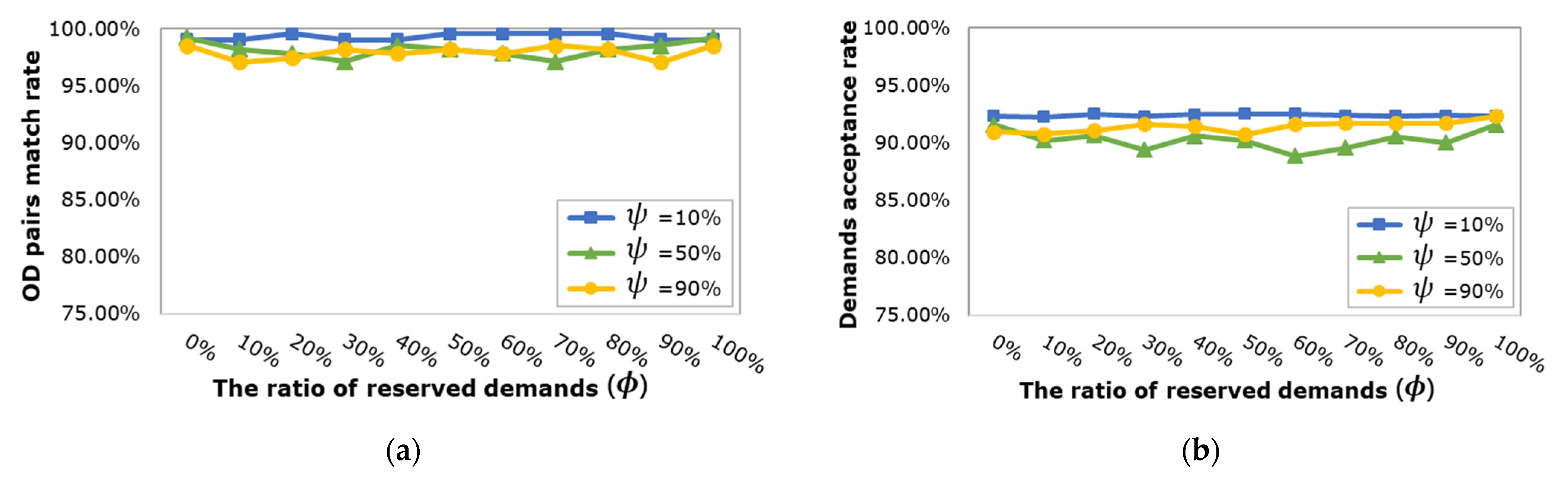
Figure 15 shows the route performance of our proposed FT in the cases with different values of and . Comparing different values of , the results under are better than the ones under . Because it is a challenge to satisfy a large number of varying dynamic-station-related demands. When , the two rates nearly remain the same with increasing, since only a small number of dynamic-station-related demands are input. When and increases from 0 to 100%, both two rates fluctuate within a narrow range. This shows that, facing a certain number of dynamic-station-related demands with random submission time, the service capacity of FT remains at a high level. When , it refers to the case that dynamic-station-related demands are all submitted before the departure date. In this case, FT achieves a larger value of demands acceptance rate, since TSPM integrates reserved demands and regular travel patterns flexibly in the first stage.
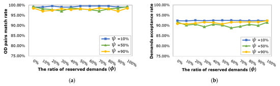
Figure 15.
Route performances in the generated cases with different values of and . The description of each panel is as follows: (a) OD pairs match rate; (b) demands acceptance rate.
To summarize, the FT proposed by MFCM and TSPM can provide good service for demands in the cases with different dynamic-station-related demands submitted at a random time, which shows its high adaptability to variations in current demands.
6. Conclusions
To bridge the gap between spatially and temporally varying demands and transportation services, FT is regarded as the feasible solution. In recent years, relevant studies have designed FT with the single-feature classification method and the base-route predesigned planning method. However, limited to a single feature, manual selection, and predesigned base routes, the FT designed by previous studies may hardly provide good service for various demands in the real world.
For the enhancement of FT’s adaptability to varying demands, this paper presents a design framework with the input of different types of demands. In terms of station classification, this paper designs MFCM based on HCA and three kinds of features. This method performs better in differences recognition than the single-feature classification method. In terms of route planning based on the results of MFCM, our study develops TSPM to generate a multi-route plan based on regular travel patterns, reserved demands, and real-time demands. Facing realistic demands, TSPM can help FT promote the demands acceptance rate compared with the base-route predesigned method. In addition, the proposed FT spends less cost and achieves higher efficiency than traditional transit. In the generated cases, the proposed FT adapts well to various demands.
In future research, the constraints of the bus volume and bus amount and the variable of the trip departure-time interval could be added to route planning models, since the bus resource is limited in reality. In addition, for the optimal plan, further optimization of the algorithm is important to support the two-stage planning method. Especially for an online plan, with the development of computer technology, the real-time traffic condition will be easily obtained, which can be used to update the arrival time of the online plan. It is also an important research direction to develop a bi-level model for designing static stations and the multi-route plan simultaneously. In addition, the proposed methods need to be tested in other areas for practical adaptability.
Author Contributions
Conceptualization, methodology, software, validation, data curation, writing—original draft preparation, formal analysis, and visualization, J.L.; resources, conceptualization, writing—review and editing, supervision, project administration, and funding acquisition, Z.H.; conceptualization, formal analysis, writing—review and editing, and supervision, J.Z. All authors have read and agreed to the published version of the manuscript.
Funding
This research was supported by “the National Natural Science Foundation of China (No. U21B2090 and No. U1811463)” and “the Fundamental Research Funds for the Central Universities, Sun Yat-sen University, 22qntd1713”.
Institutional Review Board Statement
Not applicable.
Informed Consent Statement
Not applicable.
Data Availability Statement
Not applicable.
Conflicts of Interest
The authors declare no conflict of interest.
References
- Erhardt, G.D.; Hoque, J.M.; Goyal, V.; Berrebi, S.; Brakewood, C.; Watkins, K.E. Why has public transit ridership declined in the United States? Transp. Res. Part A Policy Pract. 2022, 161, 68–87. [Google Scholar] [CrossRef]
- Bakas, I.; Drakoulis, R.; Floudas, N.; Lytrivis, P.; Amditis, A. A flexible transportation service for the optimization of a fixed-route public transport network. Transp. Res. Procedia 2016, 14, 1689–1698. [Google Scholar] [CrossRef] [Green Version]
- Angelelli, E.; Morandi, V.; Speranza, M.G. Optimization models for fair horizontal collaboration in demand-responsive transportation. Transp. Res. Part C Emerg. Technol. 2022, 140, 103725. [Google Scholar] [CrossRef]
- Militão, A.M.; Tirachini, A. Optimal fleet size for a shared demand-responsive transport system with human-driven vs automated vehicles: A total cost minimization approach. Transp. Res. Part A Policy Pract. 2021, 151, 52–80. [Google Scholar] [CrossRef]
- Nickkar, A.; Lee, Y.J.; Meskar, M. Developing an optimal algorithm for demand responsive feeder transit service accommodating temporary stops. J. Public Transp. 2022, 24, 100021. [Google Scholar] [CrossRef]
- Brake, J.; Nelson, J.D. A case study of flexible solutions to transport demand in a deregulated environment. J. Transp. Geogr. 2007, 15, 262–273. [Google Scholar] [CrossRef]
- Gorev, A.; Popova, O.; Solodkij, A. Demand-responsive transit systems in areas with low transport demand of “smart city”. Transp. Res. Procedia 2020, 50, 160–166. [Google Scholar] [CrossRef]
- Ali, A.; Ayub, N.; Shiraz, M.; Ullah, N.; Gani, A.; Qureshi, M.A. Traffic efficiency models for urban traffic management using mobile crowd sensing: A survey. Sustainability 2021, 13, 13068. [Google Scholar] [CrossRef]
- Knierim, L.; Schlüter, J.C. The attitude of potentially less mobile people towards demand responsive transport in a rural area in central Germany. J. Transp. Geogr. 2021, 96, 103202. [Google Scholar] [CrossRef]
- Cao, Y.; Jiang, D.; Wang, S. Optimization for feeder bus route model design with station transfer. Sustainability 2022, 14, 2780. [Google Scholar] [CrossRef]
- Zhang, C.; Wang, M.; Dong, J.; Lu, W.; Liu, Y.; Ni, A.; Yu, X. Factors and mechanism affecting the attractiveness of public transport: Macroscopic and microscopic perspectives. J. Adv. Transp. 2022, 2022, 5048678. [Google Scholar] [CrossRef]
- Bennich, T.; Belyazid, S. The route to sustainability—Prospects and challenges of the bio-based economy. Sustainability 2017, 9, 887. [Google Scholar] [CrossRef] [Green Version]
- Tong, L.; Zhou, L.; Liu, J.; Zhou, X. Customized bus service design for jointly optimizing passenger-to-vehicle assignment and vehicle routing. Transp. Res. Part C Emerg. Technol. 2017, 85, 451–475. [Google Scholar] [CrossRef]
- Anburuvel, A.; Perera, W.U.; Randeniya, R.D. A demand responsive public transport for a spatially scattered population in a developing country. Case Stud. Transp. Policy 2022, 10, 187–197. [Google Scholar] [CrossRef]
- Schasché, S.E.; Sposato, R.G.; Hampl, N. The dilemma of demand-responsive transport services in rural areas: Conflicting expectations and weak user acceptance. Transp. Policy 2022, 126, 43–54. [Google Scholar] [CrossRef]
- Asghari, M.; Al-e-hashem, S.M.; Rekik, Y. Environmental and social implications of incorporating carpooling service on a customized bus system. Comput. Oper. Res. 2022, 142, 105724. [Google Scholar] [CrossRef]
- Kirchhoff, P. Public transit research and development in Germany. Transp. Res. Part A Policy Pract. 1995, 29, 1–7. [Google Scholar] [CrossRef]
- Velaga, N.R.; Beecroft, M.; Nelson, J.D.; Corsar, D.; Edwards, P. Transport poverty meets the digital divide: Accessibility and connectivity in rural communities. J. Transp. Geogr. 2012, 21, 102–112. [Google Scholar] [CrossRef] [Green Version]
- Errico, F.; Crainic, T.G.; Malucelli, F.; Nonato, M. A survey on planning semi-flexible transit systems: Methodological issues and a unifying framework. Transp. Res. Part C Emerg. Technol. 2013, 36, 324–338. [Google Scholar] [CrossRef]
- Daganzo, C.F. Checkpoint dial-a-ride systems. Transp. Res. Part B Methodol. 1984, 18, 315–327. [Google Scholar] [CrossRef]
- Jaw, J.J.; Odoni, A.R.; Psaraftis, H.N.; Wilson, N.H. A heuristic algorithm for the multi-vehicle advance request dial-a-ride problem with time windows. Transp. Res. Part B Methodol. 1986, 20, 243–257. [Google Scholar] [CrossRef]
- Cordeau, J.F.; Laporte, G. A tabu search heuristic for the static multi-vehicle dial-a-ride problem. Transp. Res. Part B Methodol. 2003, 37, 579–594. [Google Scholar] [CrossRef] [Green Version]
- Diana, M.; Dessouky, M.M. A new regret insertion heuristic for solving large-scale dial-a-ride problems with time windows. Transp. Res. Part B Methodol. 2004, 38, 539–557. [Google Scholar] [CrossRef] [Green Version]
- Qiu, F.; Li, W.; Zhang, J. A dynamic station strategy to improve the performance of flex-route transit services. Transp. Res. Part C Emerg. Technol. 2014, 48, 229–240. [Google Scholar] [CrossRef]
- Zheng, Y.; Li, W.; Qiu, F. A methodology for choosing between route deviation and point deviation policies for flexible transit services. J. Adv. Transp. 2018, 2018, 6292410. [Google Scholar] [CrossRef] [Green Version]
- Zheng, Y.; Li, W.; Qiu, F. A slack arrival strategy to promote flex-route transit services. Transp. Res. Part C Emerg. Technol. 2018, 92, 442–455. [Google Scholar] [CrossRef]
- Zhang, J.; Li, W.Q.; Wang, G.Q.; Yu, J.C. Feasibility study of transferring shared bicycle users with commuting demand to flex-route transit. Sustainability 2021, 13, 6067. [Google Scholar] [CrossRef]
- Liu, X.; Qu, X.; Ma, X. Improving flex-route transit services with modular autonomous vehicles. Transp. Res. Part E Logist. Transp. Rev. 2021, 149, 102331. [Google Scholar] [CrossRef]
- Zheng, Y.; Gao, L.; Li, W. Vehicle routing and scheduling of flex-route transit under a dynamic operating environment. Discret. Dyn. Nat. Soc. 2021, 2021, 6669567. [Google Scholar] [CrossRef]
- Sun, X.; Liu, S. Research on route deviation transit operation scheduling—A case study in suburb No. 5 Road of Harbin. Sustainability 2022, 14, 633. [Google Scholar] [CrossRef]
- Qiu, F.; Li, W.; Haghani, A. An exploration of the demand limit for flex-route as feeder transit services: A case study in Salt Lake City. Public Transp. 2015, 7, 259–276. [Google Scholar] [CrossRef]
- Han, S.; Fu, H. Optimization of real-time responsive customized bus dispatch. J. Highway Transp. Res. Dev. 2020, 37, 120–127. [Google Scholar]
- Yang, H.; Cherry, C.R.; Zaretzki, R.; Ryerson, M.S.; Liu, X.; Fu, Z. A GIS-based method to identify cost-effective routes for rural deviated fixed route transit. J. Adv. Transp. 2016, 50, 1770–1784. [Google Scholar] [CrossRef]
- Otto, B.; Boysen, N. A dynamic programming based heuristic for locating stops in public transportation networks. Comput. Ind. Eng. 2014, 78, 163–174. [Google Scholar] [CrossRef]
- Huang, Z.; Liu, X. A hierarchical approach to optimizing bus stop distribution in large and fast developing cities. ISPRS Int. J. Geo-Inf. 2014, 3, 554–564. [Google Scholar] [CrossRef] [Green Version]
- Ceder, A.; Butcher, M.; Wang, L. Optimization of bus stop placement for routes on uneven topography. Transp. Res. Part B Methodol. 2015, 74, 40–61. [Google Scholar] [CrossRef]
- Johar, A.; Jain, S.S.; Garg, P.K. A conceptual approach for optimising bus stop spacing. J. Inst. Eng. India Ser. A 2017, 98, 15–23. [Google Scholar] [CrossRef]
- Cheng, G.; Zhao, S.; Zhang, T. A bi-level programming model for optimal bus stop spacing of a bus rapid transit system. Mathematics 2019, 7, 625. [Google Scholar] [CrossRef] [Green Version]
- Lyu, Y.; Chow, C.; Lee, V.; Ng, J.K.; Li, Y.; Zeng, J. CB-Planner: A bus line planning framework for customized bus systems. Transp. Res. Part C Emerg. Technol. 2019, 101, 233–253. [Google Scholar] [CrossRef]
- Liu, K.; Liu, J.; Zhang, J. Heuristic approach for the multiobjective optimization of the customized bus scheduling problem. IET Intell. Transp. Syst. 2022, 16, 277–291. [Google Scholar] [CrossRef]
- Ma, C.; Wang, C.; Xu, X. A multi-objective robust optimization model for customized bus routes. IEEE Trans. Intell. Transp. Syst. 2021, 22, 2359–2370. [Google Scholar] [CrossRef]
- Melis, L.; Sörensen, K. The real-time on-demand bus routing problem: The cost of dynamic requests. Comput. Oper. Res. 2022, 147, 105941. [Google Scholar] [CrossRef]
- Karypis, G.; Han, E.H.; Kumar, V. Chameleon: Hierarchical clustering using dynamic modeling. Computer 1999, 32, 68–75. [Google Scholar] [CrossRef] [Green Version]
- Yao, S.; Gu, M. An influence network-based consensus model for large-scale group decision making with linguistic information. Int. J. Comput. Intell. Syst. 2022, 15, 3. [Google Scholar] [CrossRef]
- Bell, J.E.; McMullen, P.R. Ant colony optimization techniques for the vehicle routing problem. Adv. Eng. Inform. 2004, 18, 41–48. [Google Scholar] [CrossRef]
- Yuan, X.; Zhang, Q.; Zeng, J. Modeling and Solution of Vehicle Routing Problem with Grey Time Windows and Multiobjective Constraints. J. Adv. Transp. 2021, 2021, 6665539. [Google Scholar] [CrossRef]


Publisher’s Note: MDPI stays neutral with regard to jurisdictional claims in published maps and institutional affiliations. |
© 2022 by the authors. Licensee MDPI, Basel, Switzerland. This article is an open access article distributed under the terms and conditions of the Creative Commons Attribution (CC BY) license (https://creativecommons.org/licenses/by/4.0/).