Article

Adoption of Micro-Mobility Solutions for Improving Environmental Sustainability: Comparison among Transportation Systems in Urban Contexts

1
Department of Civil, Architectural and Environmental Engineering, Federico II University of Naples, Via Claudio 21, 80125 Naples, Italy
2
Assosharing, Via Margutta 83, 00187 Rome, Italy
3
Helbiz Italia S.r.l., Via della Moscova 12, 20121 Milan, Italy
4
Department of Architecture, Federico II University of Naples, Via Forno Vecchio 36, 80134 Naples, Italy
*
Author to whom correspondence should be addressed.
Sustainability 2022, 14(13), 7960; https://doi.org/10.3390/su14137960
Submission received: 11 May 2022 / Revised: 24 June 2022 / Accepted: 27 June 2022 / Published: 29 June 2022

Abstract

:
Sustainable transport frameworks are gaining attention within national and international transportation policies, given the key role that decarbonisation plays in making urban environments people-friendly. Within this context, several shared services and micro-mobility options are being developed, especially as first/last mile facilities, further increasing public transport coverage levels. We present an overview of the environmental impacts of different transport modes and compare them from different perspectives, namely, CO2 emission levels, total costs (also including the user generalised cost) and service life of vehicles involved. The proposed methodology is applied to an urban context, using real trip data and showing the main findings under real conditions.

1. Introduction

Transportation systems have a crucial role to play in the quality of life and accessibility of metropolitan areas. However, they also generate externalities that affect the livability of urban environments, such as congestion, air and noise pollution. For this reason, the features of a sustainable mobility framework are at the forefront of public debate, aiming to make transport facilities environmentally friendly, whilst still being efficient and attractive for users.
Within this context, so-called push & pull policies form a key strategy. While aiming to discourage the use of private cars, they are also designed to promote public transport and other sustainable mobility options. The former goal can be achieved, for instance, by establishing restricted traffic zones or by setting appropriate parking fees. However, it is fundamental to accompany such measures with efficient public transport services; otherwise, mobility needs will remain unmet. Therefore, the necessity of a multimodal approach is clear. For this purpose, new mobility paradigms (such as alternatively powered vehicles and shared services) are becoming increasingly common and gaining substantial public interest.
In this regard, one of the main issues to be addressed is a new understanding of car use: when asked what cars are for, most would undoubtedly say that they were for moving around. Unfortunately, this response is mistaken in most urban contexts, since a car could be defined as an ornamental object, which is born to be stationary. The basis for such a provocative definition lies in the fact that, especially in urban contexts, most cars are used, at most, for 2–3 h in a day, which represents a utilization rate of lower than 15%. Hence, the main use of cars in urban areas is as stationary objects. This means that we have three alternatives:
  • Conceive and design cities as places for parked cars (parking lots rather than roads need to be built);
  • Increase the utilization of cars through car-sharing solutions (to change their primary use) and/or reduce the number of parked vehicles in urban centres by car-pooling (to increase the number of passengers carried by each vehicle);
  • Adopt micro-mobility solutions as an alternative means to cars, either directly (in the case of trips made entirely with micro-mobility vehicles) or indirectly (in the case of adduction system to increase the attractiveness of public transport with respect to private cars).
Obviously, from a sustainable perspective, the first proposal should be avoided, while the second and, especially, the third, are strongly recommended.
Within this framework, we assess the sustainability features of micro-mobility services and compare them to other mobility options from different perspectives. However, the main novelty of this paper is the use of real data on urban trips with e-scooters in a context (the city of Naples, Italy) where there are several public transport systems (buses, subways, funicular, sharing services, etc.).
The remain of the paper is organized as follows: Section 2 provides a literary review of the environmental impacts of different transport modes; Section 3 describes different perspectives that should be adopted for a fair comparative analysis; Section 4 illustrates an application to a real urban context; finally, Section 5 presents conclusions and future research insights.

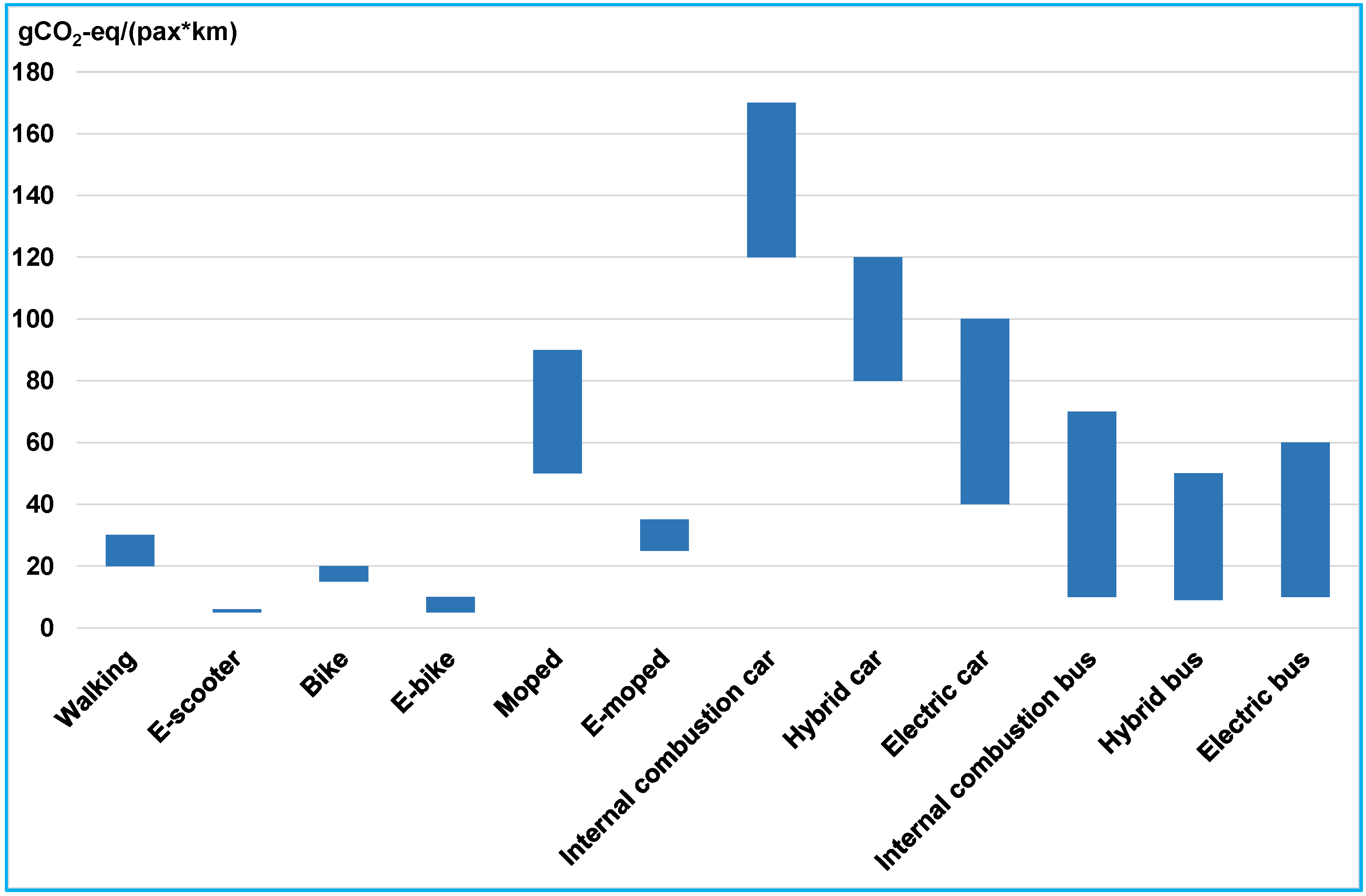
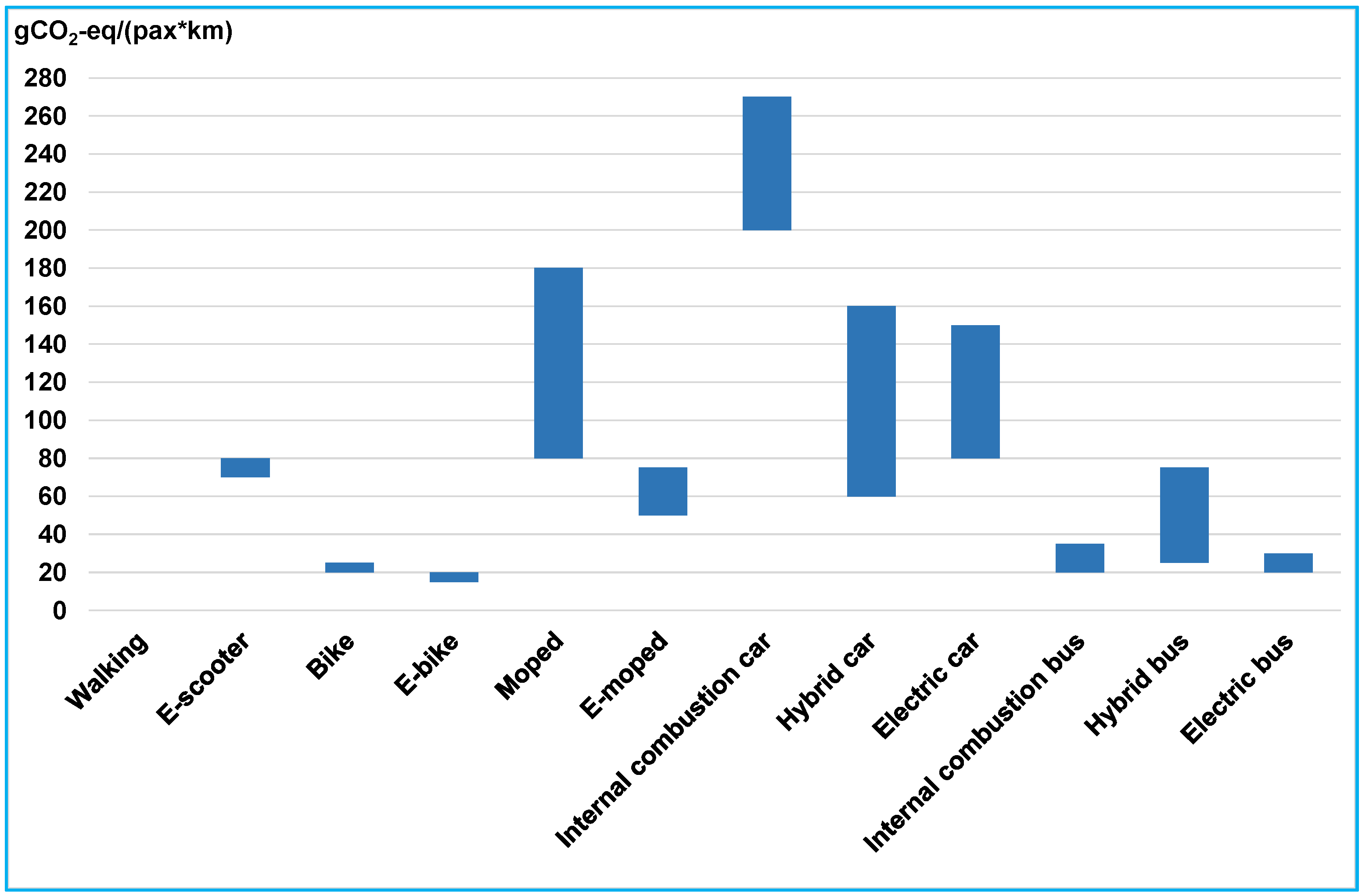
2. Literary Review on Emission Factors of Different Transport Modes

In this section, we present an assessment of the emission factors proposed in the literature in the last decade for different transport systems. First, as shown by [1], an important distinction needs to be made: emission factors can only be related to the use phase (i.e., Tank-to-Wheels (TtW)) or to the entire life-cycle (i.e., Life Cycle Assessment (LCA)) of the vehicles involved. The latter includes the production, transport and final disposal of vehicles, as well as the fuel life cycle (i.e., Well-to-Wheels (WtW)) until its end use in vehicles. Both traditional and alternatively powered transport modes have been analysed, namely, walking, cycling (conventional bike and e-bike), moped (conventional and electric), cars and buses (petrol, hybrid and electric). It is worth noting that rail systems are not involved since the reference condition is limited to an urban context where trips do not generally exceed 2 km in length [2]. Moreover, our analysis focuses on passenger transportation [3], neglecting freight modes. Various methods can be found in the literature for the emissions computation process [4,5,6,7,8,9,10,11,12,13,14]; however, in the following, the assessment of unitary emission factors proposed in the literature is discussed for each mode, and a synoptic view is finally proposed. Emission factors are expressed in terms of CO2-eq (considering the global warming impact of different greenhouse gases, such as nitrous oxide, ozone and chlorofluorocarbons) and as unit coefficients (with regard to a single passenger and a predefined unit of length, i.e., a kilometre).
As shown by [15], active modes, such as walking and cycling, cannot be defined as emission-free since they require a human physical effort and, hence, an energy expenditure. For this reason, in general, related studies refer to emissions related to the production process of the food required to cover a certain distance by walking or cycling (see, for instance, [16,17]). The European Cyclists Federation (ECF) [18] states that the average European diet is responsible for 1.44 gCO2-eq per calorie of consumed food. Therefore, given the total amount of burned calories, an estimate can be made. However, the range varies considerably, since a meat-based diet generates higher emissions than a vegetarian diet [19], and the respective speeds of pedestrians and cyclists can be very changeable [20].
Obviously, in the case of walking, there is no point talking about LCA while, in the case of the cycling mode, the emissions related to the manufacturing/disposal of the vehicles involved, i.e., conventional bikes, need to be considered when computing emissions within a life cycle assessment. According to [16], manufacturing emissions related to conventional bikes amount to 5 gCO2-eq/km, against the 7 gCO2-eq/km of an e-bike. However, this strongly depends on the kind of battery involved and the related life cycle [21]. As shown by [22], e-bikes are often used as shared services, together with other micro-mobility options, such as electric scooters, segways, hoverboards and monowheels. Micro-mobility indicates short trips with small vehicles, mainly electrically powered, which can generally host just one passenger [23]. It plays a key role, especially as a first/last mile service [24,25,26]. This allows for strong integration between different modes and leads to Mobility-as-a-Service (MaaS) scenarios where services, as well as fares, are fully integrated to the benefit of users [27,28,29,30].
With regard to e-scooter services, several papers have addressed their environmental impacts. However, few make the fundamental distinction between the analysis of emissions in the use phase and during the entire life cycle [31,32,33]. For instance, [33] made an important distinction among the different phases involved in LCA assessment and stated that a unit emission factor of 5 gCO2-eq/(pax*km) can be associated with the use phase, compared to a coefficient of 131 gCO2-eq/(pax*km) for the entire life cycle.
For motorised two-wheelers, conventional mopeds are generally compared to their electric counterparts (see, for instance, [34,35]) which, in turn, are frequently compared with other electric vehicles (see, for instance, [36,37]). Clearly, in the first case, a greener power supply plays a positive role from a sustainable perspective. By contrast, for the second comparison, the fact that electric mopeds are generally faster than e-bikes or electric micro-vehicles means that they can cover more kilometres within the same service-life duration. For instance, within the European context, ref. [38] proposed, for electric motorcycles with a displacement of 50 cc, an LCA emission factor of 76 gCO2-eq/(pax*km); this value rises to 80 gCO2-eq/(pax*km) in the case of greater displacements. On the other hand, for conventional mopeds of the same displacement, the paper shows an LCA emission factor of 85 gCO2-eq/(pax*km) and 175 gCO2-eq/(pax*km), respectively. Indications of the emission factors that are limited to the operating phase can be found in [39].
In the case of cars and buses, hybrid solutions have also been considered. As shown by [40], the flexibility and convenience of using private cars are hard to achieve with other transport modes. Therefore, finding a greener power supply for such a solution proves fundamental. For instance, [1] proposed an LCA emission factor for hybrid and electric cars of around 150 gCO2-eq/(pax*km), which rises to 260 gCO2-eq/(pax*km) in the case of internal combustion vehicles. As shown by [41], in the case of electric cars, amongst others, issues of charging time, lack of charging infrastructure and single-fuelling travel range (in terms of kilometres) need to be addressed. Noteworthy discussions on trends and future developments in the case of hybrid and electric cars can be found in [42,43].
Finally, regarding transit systems, the most promising scenario is based on the adoption of e-fleets, which are frequently associated with fully automated management frameworks [44,45,46,47]. Noteworthy estimates of related emission factors can be found in [48,49]. However, the higher carrying capacity of buses reduces the value of CO2 emissions per individual user. For instance, according to [38], an LCA factor emission of 260 gCO2-eq/(pax*km) can be estimated for electric cars, against a value of 25.7 gCO2-eq/(pax*km) for e-buses.
An overview of the above literature is shown in Table 1. where, for each analysed transport mode, a range of emission factors is presented, distinguishing only between the use phase and the entire life cycle assessment. Likewise, Figure 1 and Figure 2 provide a synopsis of the identified ranges in the case of the operating phase and entire life cycle assessment, respectively.
However, focusing only on the emissions provided by each transport mode provides a partial perspective of the sustainability of each mobility system. Therefore, in the following, different comparison criteria are proposed, providing a fairly comprehensive analysis.
The analysis of the data shown in Table 1 and Figure 1 and Figure 2 shows that the occupancy coefficient plays a fundamental role in defining the environmental impacts of transportation systems. Indeed, cars have the worst performance in terms of gCO2-eq/(pax*km) emissions, even in the case of hybrid or electric vehicles. Similarly, a bus has less impact due to the high number of people that are transported, even in the case of an internal combustion engine.

3. Methodologies for Comparing Transportation Systems in a Sustainable Perspective

Comparing different transport modes by considering only relative emissions yields a biased analysis of the degree of sustainability associated with each mobility system. For this reason, three different criteria are proposed to perform a comprehensive and accurate comparison of urban transport systems from a sustainable perspective.
The first criterion is the most widely used and concerns the level of emissions. However, as was previously pointed out, a key distinction needs to be made between the sole use phase of a certain vehicle and its entire life cycle. For instance, electrically powered modes can be defined by their having zero local emissions. However, electric vehicles, as well as the electricity required to run them, need to be produced, which greatly affects their environmental impact. Furthermore, in the case of shared services, a particular phase needs to be considered, i.e., the process including pick-up for charging, actual charging and re-positioning of the vehicles. As shown by [32], this phase can account for 40% of the total emissions of a shared mode. Therefore, to provide an accurate comparison of the different transport systems, the above amount should be neglected. In this case, the emission factors shown in Table 1 are considered. As mentioned above, they are expressed in terms of CO2-eq and pertain to an individual passenger and a predefined unit of length. In this way, given the carrying capacity of each vehicle, as well as the spatial patterns covered by trips made with different modes, total emissions can be derived, thus providing a fair comparative analysis. In particular, for each analysed transport mode, it can be stated that:
TEm = ζm · dm · nm
where TEm is total emissions related to mode m; ζm is the unit emission factor for mode m; dm is the distance covered by each trip undertaken with mode m; nm is the number of trips undertaken with mode m.
The second criterion consists of considering the total cost associated with a specific transport mode. This can be defined, for each transport mode m, as the sum between externalities (expressed in monetary terms) and the user-generalised cost, as shown below:
TCm = ECm + UGCm
where TCm is the total cost related to mode m; ECm is the cost associated with the externalities produced by mode m; UGCm is the user-generalised cost related to mode m.
Externalities generally include the side effects related to a certain transport mode (such as air and noise pollution, accidents, etc.); in our case, we focused on CO2 emissions. Therefore, value ECm can be obtained by expressing the total emissions TEm computed through Equation (1) for that specific transport mode in monetary terms. By contrast, user-generalised cost is considered as the sum of time rates and monetary costs that a user incurs to undertake a certain trip. Travel time rates must be considered in all cases, with different orders of magnitude according to the speeds involved. Other quantities also need to be determined according to the specific transport system being analysed. Typically, in the case of a transit system, in addition travel times, access/egress times (for reaching/leaving the stop), waiting times (waiting for the approaching bus) and fares have to be considered. The space–time continuity of private cars causes the above additional time rates to equal zero; however, in this case, parking charges need to be added and rental costs have to be considered in the case of shared vehicles. In light of the above, a total cost approach provides a more realistic comparative view, enriching the analysis with a passenger-oriented perspective. This is a crucial factor, since each transport system is not an end in itself, but its prime aim is to transport people (and goods).
The third approach aims to provide a synoptic indicator that describes the sustainability level of a certain transport system by also considering the relative mass and service life duration, i.e.,
Im = MVm/SLm
where Im is the KPI related to mode m; MVm is the mass associated with the vehicle used in the case of mode m; and SLm is the service life of the vehicle used in the case of mode m.
These two elements (i.e., mass and the service life of the adopted vehicle) are both crucial for considering emission levels. Clearly, the larger the vehicle, the more burdensome the production, transport and disposal phases. Moreover, according to Newton’s well-known laws of motion [50], to move a greater mass, we need more power. In the case of electric vehicles, this means producing, and ultimately disposing of, batteries. Further, it is clear that, when higher speeds are allowed, the vehicle in question can cover more kilometres, its service life being equal.
Finally, a further indicator is introduced, namely, I′m, which can be obtained by scaling the synthetic indicator Im according to the carrying capacity CCm associated with the vehicle used for mode m, that is:
I′m = Im/CCm
Considering the carrying capacity of transport modes allows us to make our analysis more accurate and avoids a biased outcome, as will be shown in the application section.

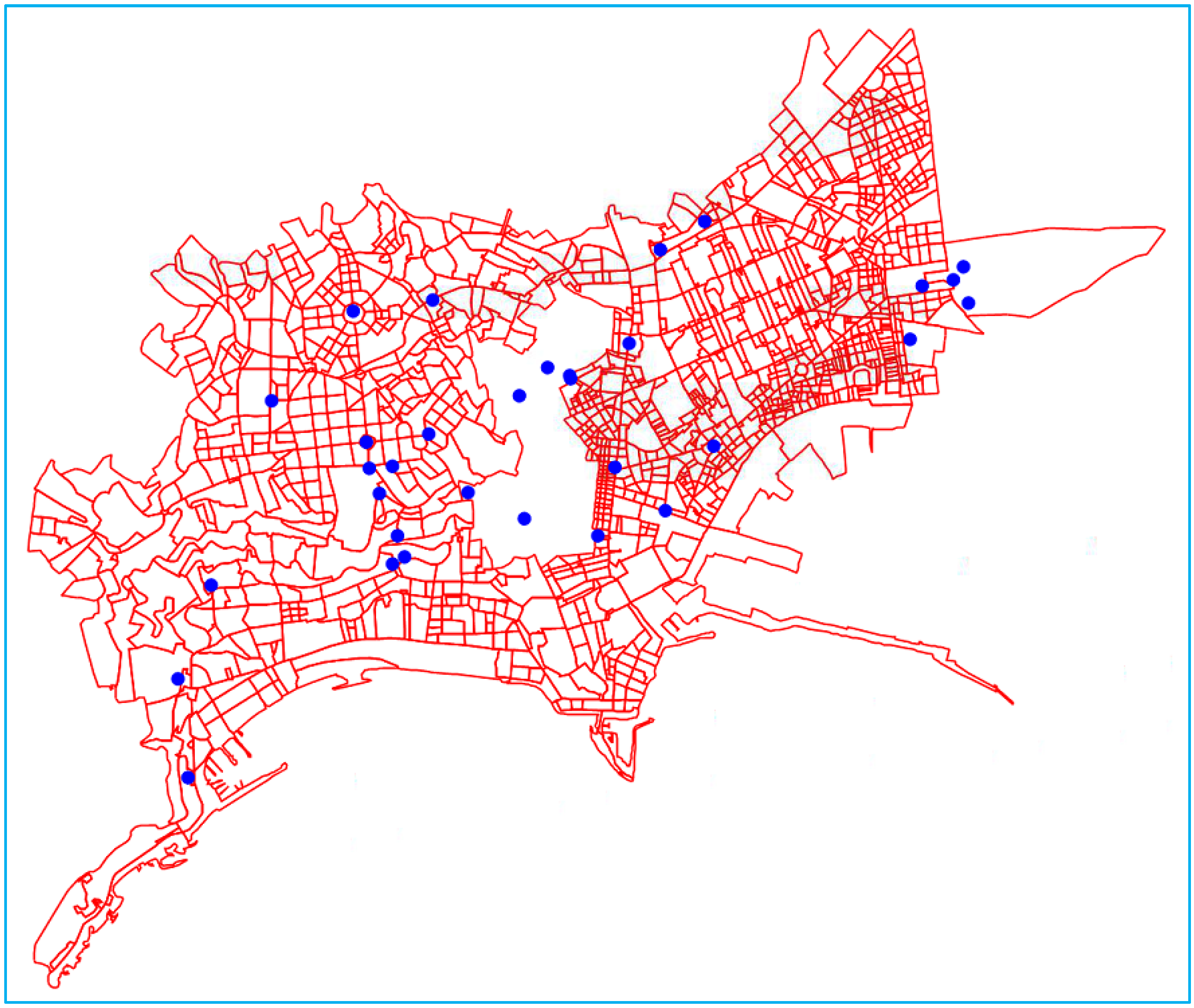
4. Application to a Real Urban Context

To show the feasibility of the proposed approach, it was applied to a real urban context, i.e., the city of Naples, in southern Italy. The application was implemented in two phases:
  • Phase 1: one or more models were set up to describe user behaviour in terms of e-scooter trips;
  • Phase 2: the environmental performance of e-scooters was compared to that of other transportation systems.
All analyses were implemented with the e-scooter choice as a benchmark indicator.
Figure 3 shows the analysed area, which is represented by the city centre, where census tracts are reported as red-bordered areas and public transport (rail, underground and funicular) stations as blue points.

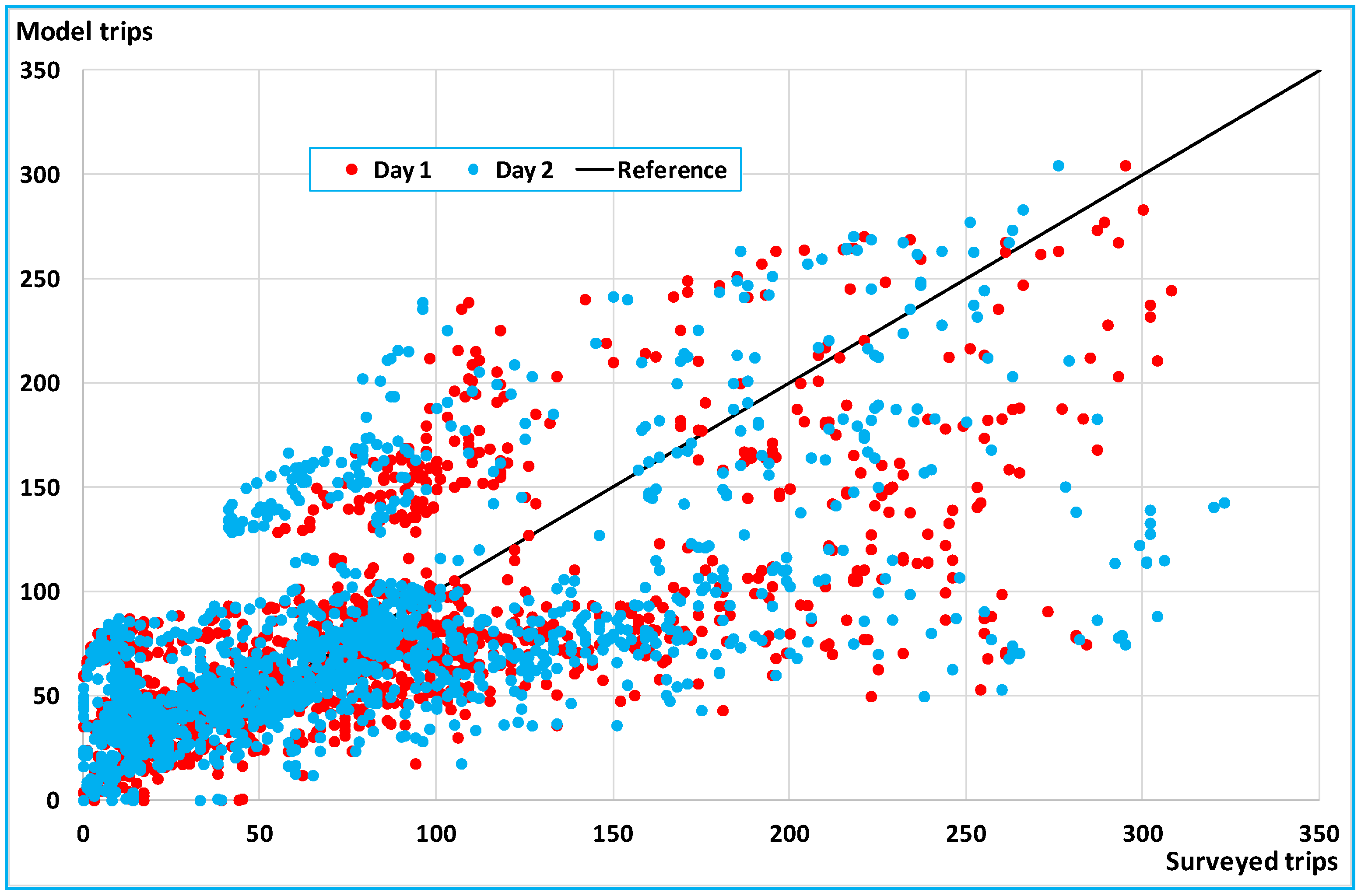
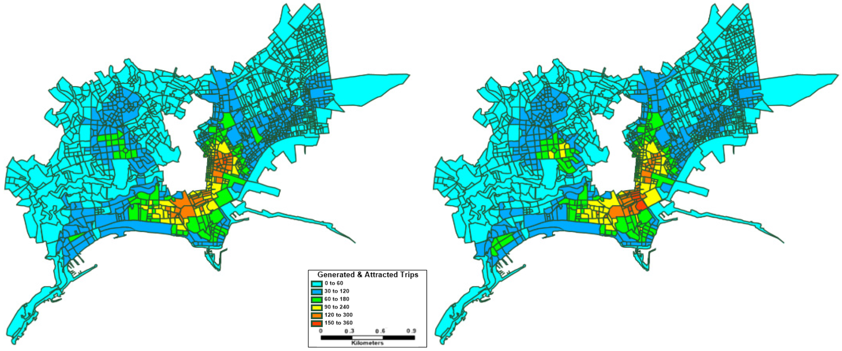
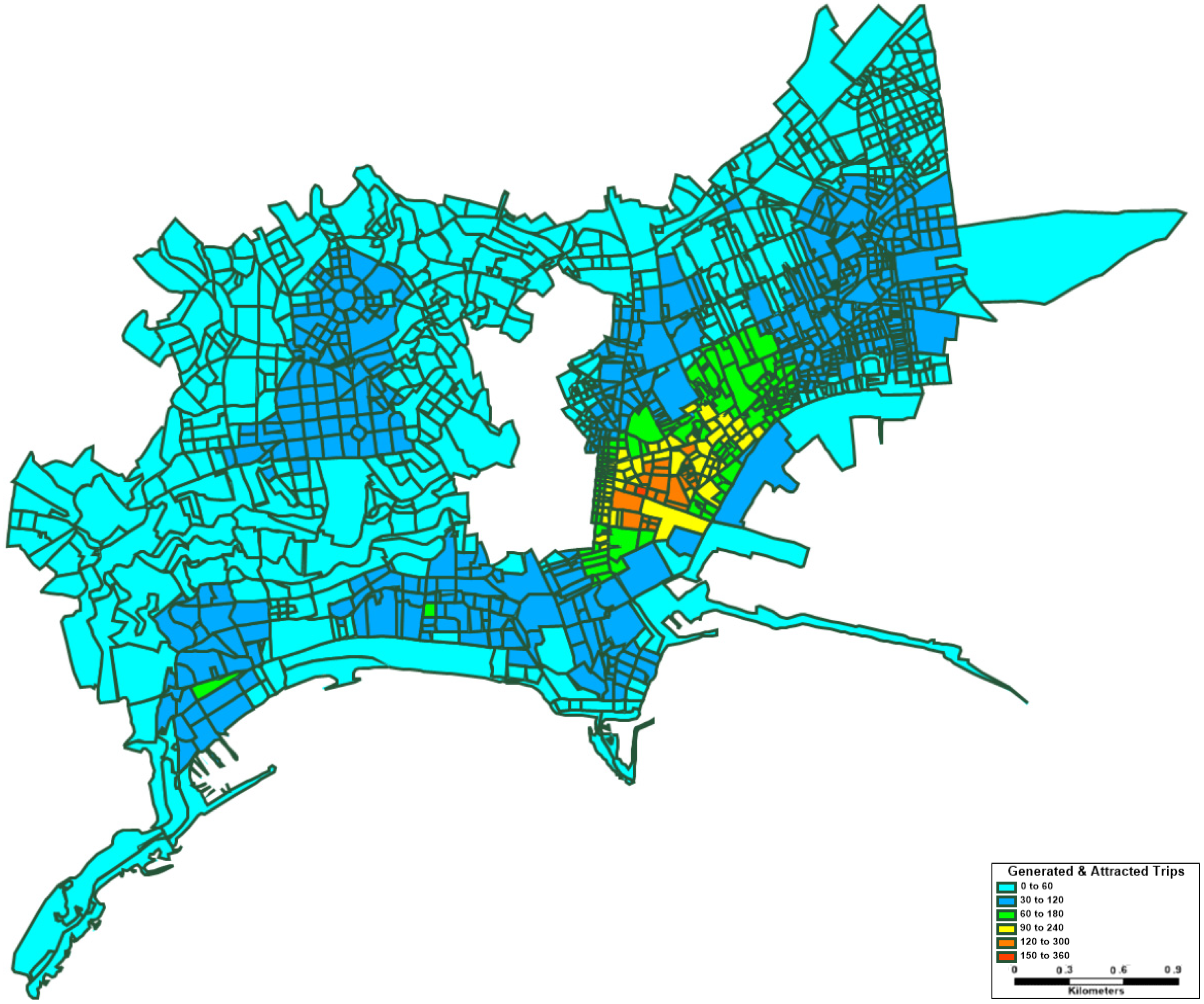
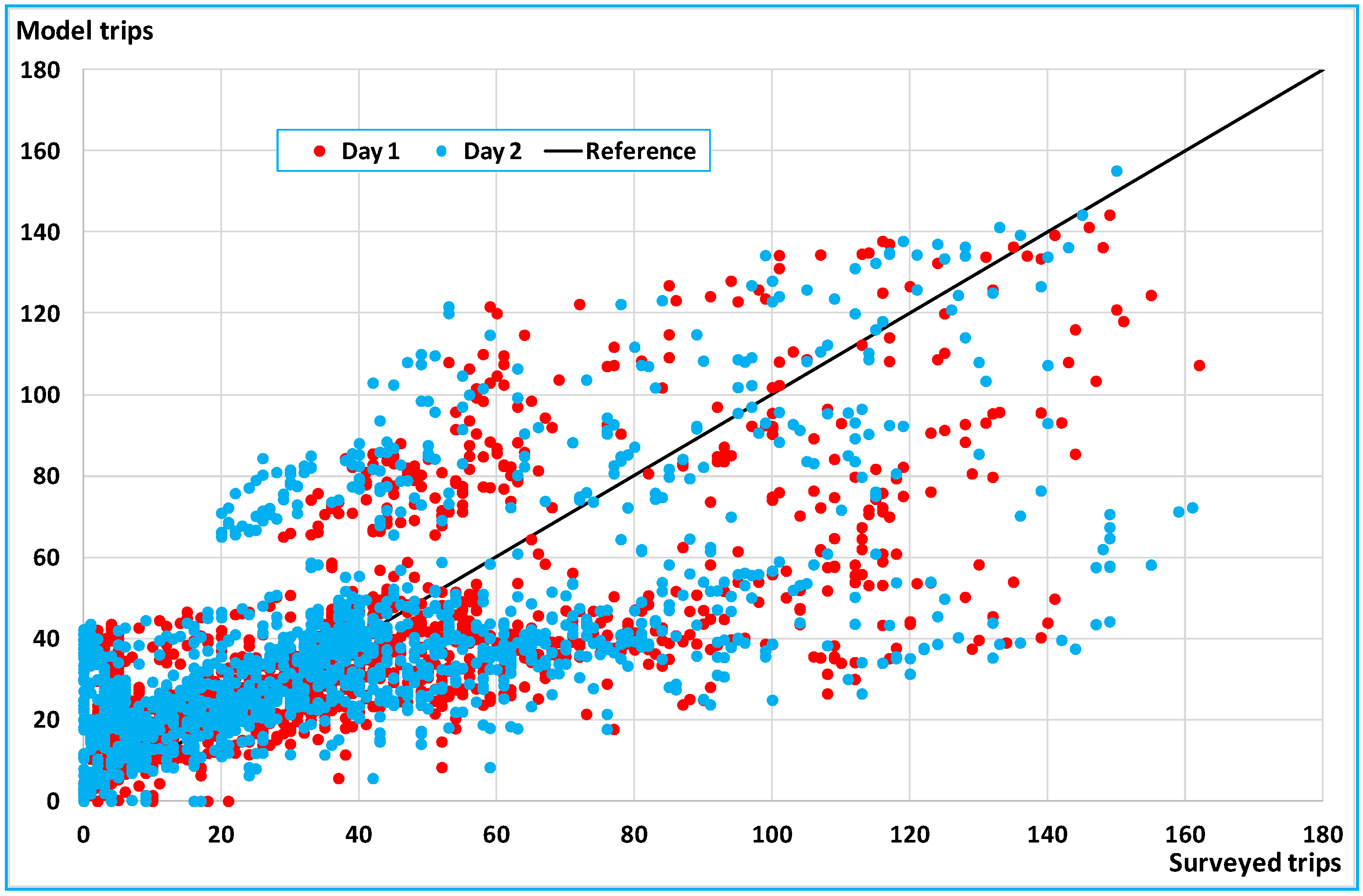
4.1. Model Definition to Describe User Behaviour

To set up one or more models to describe the behaviour of users travelling by e-scooter, we analysed real data concerning user trips. The data were obtained from an e-scooter rental company in Naples. They refer to two consecutive working days with similar weather conditions. Below, we will conventionally identify these days as Day 1 and Day 2.
To build a robust model and verify its reproducibility, we used the Day 1 data to calibrate the models (i.e., to build models capable of reproducing the surveyed data) and those of Day 2 for validation (i.e., to verify how well the models are able to “predict” the data from Day 2).
The calibration task of a model may be divided into three phases: specification, calibration and validation. The validation task of a model is identified by a single phase: validation. Although tasks and phases may have the same terms (i.e., calibration task and calibration phase, or validation phase and validation task), they represent different steps in the procedure to build a robust model.
However, in the case of the calibration task, the specification phase consists of defining the functional form of the model, the input and output variables. The calibration phase entails identifying the numerical values of the coefficients of the function identified in the specification phase. Finally, the validation phase consists of determining whether the model is able to reproduce the physical phenomenon described by the data used for calibration (in this application, the data from Day 1).
Likewise, in the case of the validation task, the validation phase consists of checking whether the model calibrated using a database (for instance, Day 1 data) is able to reproduce a different database (for instance, Day 2 data).
By adopting the above procedure, after numerous attempts, we determined three models that could describe the behaviour of users travelling by e-scooter. First of all, it is necessary to establish the pedestrian influence area of a census tract as the circular area with a radius of 300 metres (corresponding to the distance travelled in 5 min at a pedestrian speed of 1 m/s), with the census tract as its centre. According to this definition, the first model provides the daily number of trips generated by a census tract according to the following formula:
N_Geni = α1 · N_Resi + α2 · N_Empi + α3 · Dist_Stationi
where N_Geni is the number of e-scooter trips generated in the pedestrian influence area of the i-th census tract; N_Resi is the number of residents in the pedestrian influence area of the i-th census tract; N_Empi is the number of employees in the pedestrian influence area of the i-th census tract; Dist_Stationi is the distance (expressed in metres) of the census tract centre from the nearest public transport station; α1, α2 and α3 are the three parameters that are to be calibrated.
Likewise, the second model provides the daily number of trips attracted by a census tract according to the following formula:
N_Attri = β1 · N_Resi + β2 · N_Empi + β3 · Dist_Stationi
where N_Attri is the number of e-scooter trips attracted in the pedestrian influence area of the i-th census tract; β1, β2 and β3 are the three parameters that are to be calibrated.
Finally, the third model provides the daily number of trips generated or attracted by a census tract according to the following formula:
N_Tripsi = γ1 · N_Resi + γ2 · N_Empi + γ3 · Dist_Stationi
where N_Tripsi is the number of e-scooter trips generated or attracted in the pedestrian influence area of the i-th census tract; γ1, γ2 and γ3 are the three parameters that are to be calibrated.
As the third model may be expressed as the sum of the two previous models, that is,
N_Tripsi = N_Geni + N_Attri
it may be stated that:
γ j = α j + β j      ∀ j ∈ {1, 2, 3}
However, although the specification and calibration phases may be superfluous for the third model, the validation phases give rise to results that cannot be expressed as the sum of the performances achieved in the first two models.
The three proposed models express the same phenomenon from different perspectives. By providing the number of trips generated by an area (emission model), the first model expresses the tendency to use e-scooters to reach neighbouring areas. The results of the first model may be adopted as a proxy value of the active accessibility (i.e., the ability/easiness of reaching neighbouring areas).
Similarly, the second model, by providing the number of trips attracted to an area (attraction model), expresses the tendency to use e-scooters to be reached from neighbouring areas. The result of this model may be adopted as a proxy value of the passive accessibility (i.e., the ability/ease of being reached from neighbouring areas).
Since in real cases there are not only emission zones or only attractive zones (there could be zones with mixed behaviours), and some movements could use the e-scooter for both the outward and return trips, a third model has been proposed, which can be expressed as a sum of the previous ones, considering both the areas with a mixed vocation (emission plus attraction) and the outward and return trips.
Details of the calibration and validation tasks are given in Table 2, Table 3 and Table 4, and Figure 4, Figure 5 and Figure 6 provide a comparison of the surveyed trips (real data) and model trips (estimated data) in terms of a scatter plot graph, both for Day 1 (calibration data) and Day 2 (validation data). Function tests (i.e., R2, R2adj and F-test) in Table 2, Table 3 and Table 4 provide the numerical description (i.e., performance) of Figure 4, Figure 5 and Figure 6.
Model outcomes in terms of trips can be represented in terms of heat maps. For each model, the real data from Day 1 (calibration data), the real data from Day 2 (validation data) and model data (estimated trips) were compared. A comparison of the heat maps shows that:
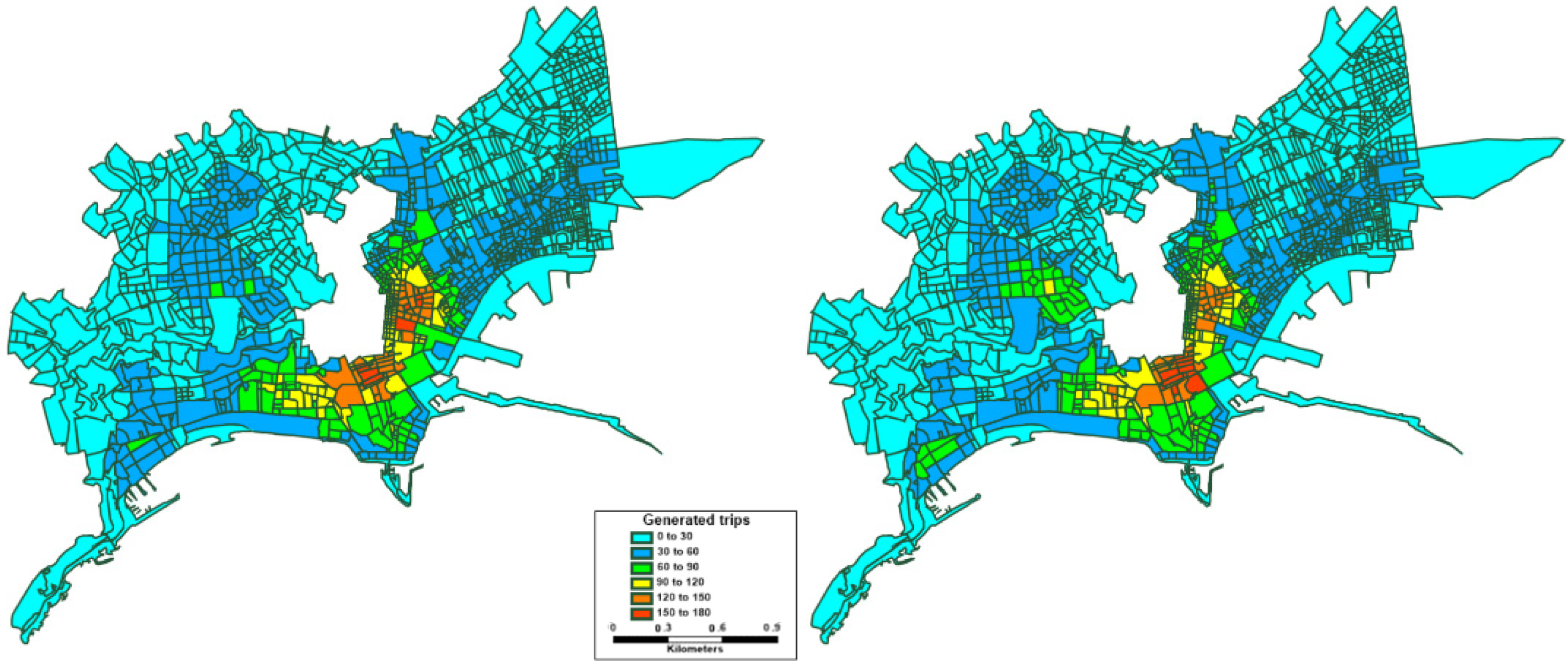
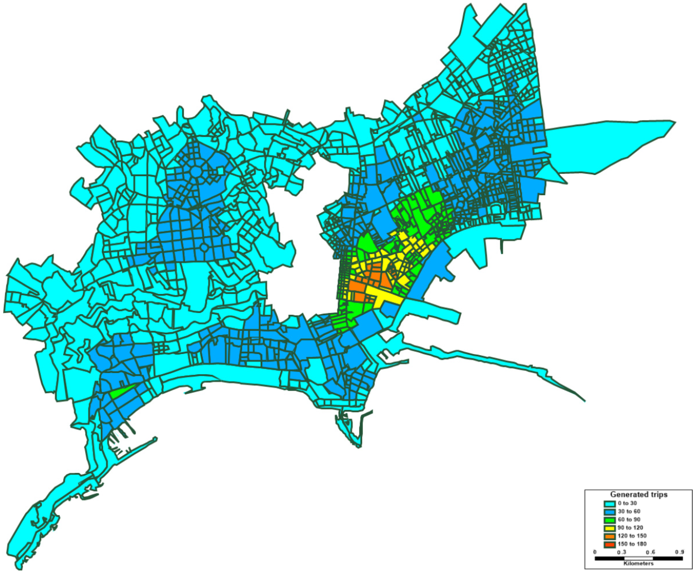
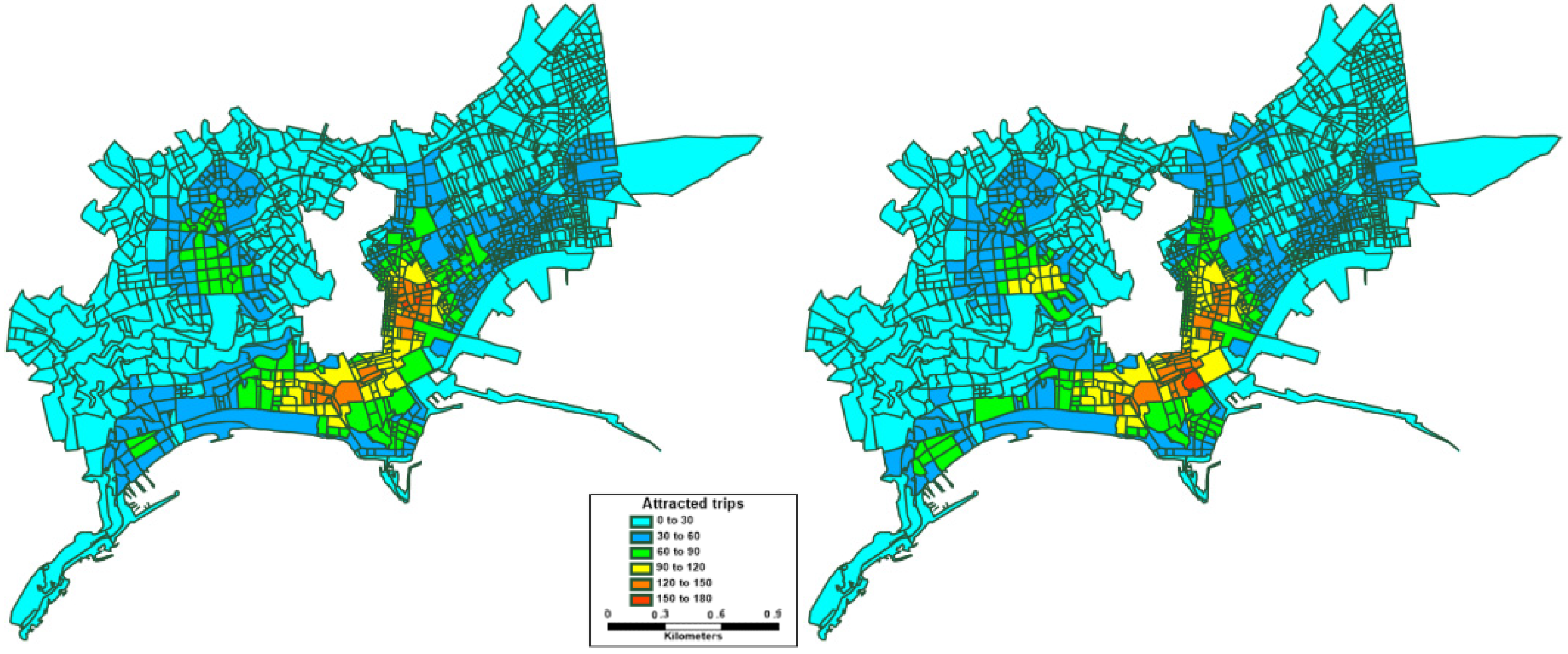
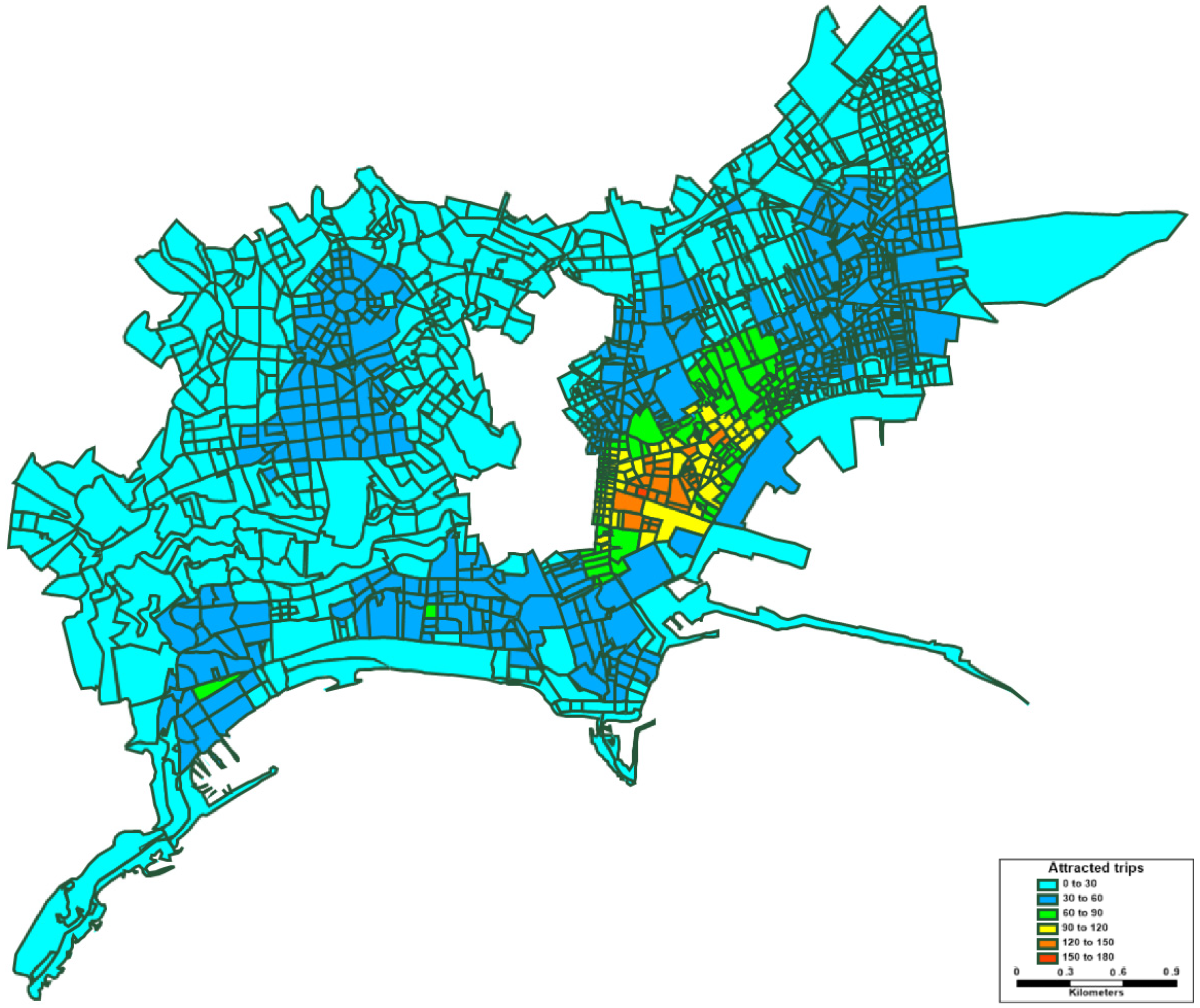
  • Day 1 real data are very similar to those of Day 2, as they were similar days in terms of weather conditions, which provides a similar value of trips in terms of both quantity (number of trips) and distribution (trip density).
  • The model data reproduce both Day 1 data (calibration data) and Day 2 data (validation data) well, confirming the heat maps’ ability to reproduce the physical phenomenon.
The heat maps representing real and model data in the case of the daily number of trips generated by census tracts (i.e., Model 1) are shown in Figure 7 and Figure 8. Likewise, heat maps representing real and model data in the case of the daily number of trips attracted by census tracts (i.e., Model 2) are shown in Figure 9 and Figure 10. Finally, heat maps representing real and model data in the case of the daily number of trips generated or attracted by census tracts (i.e., Model 3) are shown in Figure 11 and Figure 12.
The analysis of the heat maps (Figure 7, Figure 8, Figure 9, Figure 10, Figure 11 and Figure 12) confirms what was anticipated with the scatter plots (Figure 4, Figure 5 and Figure 6), i.e., Day 1 and Day 2 are very similar, and the developed models can reproduce both the calibration data (Day 1) and validation data (Day 2).
Obviously, since the meteorological conditions are similar in the examined days, the model could not capture the variability in the use of e-scooters depending on meteorological factors, and could only capture the variability in static factors such as the number of residents, the number of employees and the distance from the stations of the public transport.
In particular, the presence of a negative coefficient associated with distance from the stations (i.e., the greater the distance, the lower the propensity to use e-scooters) highlights the tendency to use e-scooters not only for monomodal trips (i.e., those made entirely by e-scooter) but also for multimodal trips where the e-scooter represents a system of adduction to public transport.
These data ire extremely relevant as they identify scooters as a possible tool to increase the area of influence of public transport, thereby increasing its attractiveness.

4.2. Comparison among Transport Modes

Given the total amount of kilometres covered and a specific occupancy coefficient according to the analysed mode, through Equation (1), we may compute total emissions, both for the entire life cycle and only the use phase, for each assessed transport system. The only exception is the walking mode for which, as already noted, there is no point discussing LCA.
Related results are shown, respectively, in Table 5 and Table 6, for both days in question. Red values show less sustainable modes while green values indicate the most environmentally friendly systems.
Due to the linearity of Equation (1), computed total emissions basically follow the conceptual outcome of the unit factors derived from the literature review. For electric modes, e-bikes emerge as being more sustainable than e-scooters, due to the option of pedal assistance. However, the impact of e-mopeds is comparable to that of e-scooters, despite the greater mass that has to be moved. This is due to the higher speeds that an e-moped can reach, leading to a greater distance being covered during its service life. The highest impact is generated by cars, especially internal combustion vehicles. This is due to the fact that congestion limits the speeds that can be attained by cars in urban environments. Finally, the low impact shown for buses is due to the high carrying capacity involved, which generates a very low unit emission coefficient (i.e., gCO2/pax).
Moving onto the second criterion, the total cost of each mode was computed by considering data from Day 1, with a total distance of 2411 km and 1665 trips being undertaken. First, total emissions are expressed as monetary costs, i.e., in Euros, according to [39] and considering a unit cost of 0.20 €/kWh. The user generalised cost for each mode is computed and added to the externalities, thus obtaining the total cost according to equation (2). In particular, the following assumptions are made. Travel times are obtained according to the average speed estimated for each vehicle. Additional times are then computed according to the mode in question, that is: (i) the average time spent looking for an available parking slot in the case of mopeds and cars (5 and 15 min, respectively); (ii) average waiting times at the bus stop (20 min) in the case of transit systems. Each value, expressed as a time measure, is multiplied by a Value of Time (VOT) of €5/h, thus obtaining the relative monetary value. Finally, the monetary costs involved are considered, that is: (i) for e-scooters, e-bikes and mopeds, a fixed rental rate of €0.50 for each trip is taken into account; (ii) for cars, a parking fee of €5 is introduced; (iii) for buses, the fare is added for each run (€1.10).
The results are shown in Table 7, where red percentages show more expensive modes, green values indicate less expensive modes and the orange value represents an intermediate condition. The latter refers to walking which, against a small environmental impact, has the great drawback of a much longer travel time w.r.t. other transport modes, when the distance to be covered is equal.
Private cars still fall within the red zone, since both externalities and user-generalised costs are very high. In this case, the bus mode falls within the same zone. Indeed, although more sustainable (i.e., low externalities), the transit system is penalised by the intrinsic temporal–spatial discontinuity by which it is characterised. The latter generates access/egress times and waiting times at stops, which drive up the related user-generalised cost. In the green zone, instead, we find e-scooters and e-bikes, followed by conventional bikes and mopeds. Clearly, this holds for urban contexts while, when there are greater distances to be covered, this framework could be inverted in favour of cars and buses.
Finally, according to Equations (3) and (4), synthetic indicators Im and I′m are computed. They consider the mass and service life of the vehicles concerned. Such variables are crucial since, as previously mentioned, the greater the vehicle mass, the more burdensome the production, transport and disposal phases, and the greater the power needed. Moreover, when higher speeds are allowed, the vehicle in question can cover more kilometres, with the service life being equal. The ratio between mass and service life of the vehicle with reference to the single user, i.e., I′m, is also a meaningful measurement, as it considers the carrying capacity of the vehicles involved.
The results are summarised in Table 8, where red values show the worst options, green values indicate the best modes and orange values represent intermediate conditions. Due to their mass, cars and buses fall within the red zone, followed by mopeds. By contrast, despite its brief service life, the e-scooter falls within the less impactful systems, after bikes, showing a mass/service life ratio of about 1 to 7 with respect to internal combustion and hybrid cars, which becomes about 1 to 11 with respect to electric cars. Finally, it is worth noting that, for a single passenger, buses recover ground, once again thanks to their carrying capacity, which significantly exceeds that of other transport systems.
A relevant result is that the vehicle-occupancy coefficient plays a fundamental role in the definition of unitary emissions. Therefore, even in the case of an internal combustion engine, a bus is always more environmentally friendly than a car, even if the car is hybrid or electric.
Obviously, a different case would occur when a bus travels with a low occupancy level or, worse, is completely empty. In this case, however, this would be a planning error in the designed service because, if the bus travels empty, this means that it is useless and, therefore, in addition to polluting, it absorbs and wastes the economic resources of the community.

5. Conclusions and Research Prospects

In conclusion, the paper provides a three-fold methodology for carrying out a fair comparison of different transport modes within urban contexts. The aim was to avoid a biased assessment, which, by neglecting some important elements, could lead to an unrealistic and inaccurate outcome.
First, the importance of distinguishing vehicle emissions related only to the use phase with respect to the entire life cycle was stated. The emission factors obtained from the literary review fully support this principle. Secondly, a total-cost approach was proposed, thus enriching the comparison with a user-oriented perspective. Finally, synthetic indicators, considering vehicle mass and service life, were proposed. The outcome clearly shows the presence of different evaluation criteria and, hence, the lack of a mode that is the optimal option in any condition. However, in an urban environment, e-scooters, together with active modes, display several advantages, especially regarding first/last mile services and Park & Ride solutions. These data are also highlighted by the fact that, in all calibrated models, the distance from public transport stations was significant.
Finally, the proposed model could also be used to define the greatest concentration of demand for e-scooters in order to identify where to locate the charging points, possibly based on the use of photovoltaic panels, as suggested by [51].
In terms of future research, we propose to perform the same comparison in other urban contexts, and also in rural contexts, thus extending the assessment to other transport modes, such as rail. Finally, it would be interesting to apply the proposed approach in the case of a Mobility-as-a-Service scenario, where the total cost is greatly affected by the presence of shared modes and the degree of integration among different transport services and related fares.

Author Contributions

Conceptualization, L.D., L.P., M.T. and S.C.; data curation, C.T., L.P., M.B. and L.D.C.; formal analysis, L.D., L.P. and M.B.; investigation, C.T., L.D., L.P., M.B. and L.D.C.; methodology, L.D., L.P. and M.B.; validation, L.D., L.P. and M.B.; data curation, C.T., L.P., M.B. and L.D.C.; supervision, L.D., L.P. and M.T.; writing—original draft, C.T., L.D., L.P., M.B., L.D.C., M.T. and S.C.; writing—review and editing, C.T., L.D., L.P., M.B., L.D.C., M.T. and S.C. All authors have read and agreed to the published version of the manuscript.

Funding

This research was partially funded by Federico II University of Naples (Italy), grant number 000009-ALTRO-R-2022-LD “Department research DICEA”.

Institutional Review Board Statement

Not applicable.

Informed Consent Statement

Not applicable.

Data Availability Statement

The data used to support the findings of this study are available from the corresponding authors upon request.

Conflicts of Interest

The authors declare no conflict of interest. The funders had no role in the design of the study; in the collection, analyses, or interpretation of data; in the writing of the manuscript, or in the decision to publish the results.

References

  1. Ma, H.; Balthasar, F.; Tait, N.; Riera-Palou, X.; Harrison, A. A new comparison between the life cycle greenhouse gas emissions of battery electric vehicles and internal combustion vehicles. Energy Policy 2012, 44, 160–173. [Google Scholar] [CrossRef]
  2. Brunner, H.; Hirz, M.; Hirschberg, W.; Fallast, K. Evaluation of various means of transport for urban areas. Energy Sustain. Soc. 2018, 8, 9. [Google Scholar] [CrossRef] [Green Version]
  3. Chester, M.; Horvath, A. Environmental Life-Cycle Assessment of Passenger Transportation: A Detailed Methodology for Energy, Greenhouse Gas and Criteria Pollutant Inventories of Automobiles, Buses, Light Rail, Heavy Rail and Air; Working Paper UCB-ITS-VWP-2008-2; UC Berkeley Center for Future Urban Transport: Berkeley, CA, USA, 2008; Available online: https://escholarship.org/uc/item/5670921q (accessed on 10 June 2021).
  4. Lents, J.; Canada, M.; Nikkila, N.; Tolvett, S. Measurement of in-Use Passenger Vehicle Emissions in Almaty, Kazakhstan; ISSRC Report; ISSRC: La Habra, CA, USA, 2007; Available online: http://www.issrc.org/ive/downloads/reports/AlmatyKazakhstan2007.pdf (accessed on 10 June 2021).
  5. Chester, M.V.; Horvath, A. Environmental assessment of passenger transportation should include infrastructure and supply chains. Environ. Res. Lett. 2009, 4, 024008. [Google Scholar] [CrossRef]
  6. Ntziachristos, L.; Gkatzoflias, D.; Kouridis, C.; Samaras, Z. COPERT: A European road transport emission inventory model. In Information Technologies in Environmental Engineering. Environmental Science and Engineering; Athanasiadis, I.N., Rizzoli, A.E., Mitkas, P.A., Gómez, J.M., Eds.; Springer: Berlin/Heidelberg, Germany, 2009; pp. 491–504. [Google Scholar] [CrossRef]
  7. Del Pero, F.; Delogu, M.; Pierini, M.; Bonaffini, D. Life Cycle Assessment of a heavy metro train. J. Clean. Prod. 2015, 87, 787–799. [Google Scholar] [CrossRef]
  8. Girardi, P.; Gargiulo, A.; Brambilla, P.C. A comparative LCA of an electric vehicle and an internal combustion engine vehicle using the appropriate power mix: The Italian case study. Int. J. Life Cycle Assess. 2015, 20, 1127–1142. [Google Scholar] [CrossRef]
  9. Aly, S.H.; Ramli, M.I. A Development of MARNI 12.2 model: A calculation tool of vehicular emission for heterogeneous traffic conditions. J. Eng. Appl. Sci. 2016, 11, 43–50. [Google Scholar] [CrossRef]
  10. Kholod, N.; Evans, M.; Gusev, E.; Yu, S.; Malyshev, V.; Tretyakova, S.; Barinov, A. A methodology for calculating transport emissions in cities with limited traffic data: Case study of diesel particulates and black carbon emissions in Murmansk. Sci. Total Environ. 2016, 547, 305–313. [Google Scholar] [CrossRef] [Green Version]
  11. Jones, H.; Moura, F.; Domingos, T. Life cycle assessment of high-speed rail: A case study in Portugal. Int. J. Life Cycle Assess. 2017, 22, 410–422. [Google Scholar] [CrossRef]
  12. Mellino, S.; Petrillo, A.; Cigolotti, V.; Autorino, C.; Jannelli, E.; Ulgiati, S. A Life Cycle Assessment of lithium battery and hydrogen-FC powered electric bicycles: Searching for cleaner solutions to urban mobility. Int. J. Hydrogen Energy 2017, 42, 1830–1840. [Google Scholar] [CrossRef]
  13. Cox, B.L.; Mutel, C.L. The environmental and cost performance of current and future motorcycles. Appl. Energy 2018, 212, 1013–1024. [Google Scholar] [CrossRef]
  14. Aly, S.H.; Ramli, M.I.; Arifin, Z. Estimation of carbon dioxide emissions on heterogeneous traffic based on metropolitan traffic emissions inventory model. GEOMATE J. 2021, 21, 181–190. [Google Scholar] [CrossRef]
  15. Mizdrak, A.; Cobiac, L.J.; Cleghorn, C.L.; Woodward, A.; Blakely, T. Fuelling walking and cycling: Human powered locomotion is associated with non-negligible greenhouse gas emissions. Sci. Rep. 2020, 10, 9196. [Google Scholar] [CrossRef] [PubMed]
  16. Stott, S. How green is cycling? Riding, walking, ebikes and driving ranked. Bikeradar 2020. Available online: https://www.bikeradar.com/features/long-reads/cycling-environmental-impact (accessed on 10 June 2021).
  17. Handy, S. Want to save tons of greenhouse gases? Bike it. Sci. Clim. 2018. Available online: https://climatechange.ucdavis.edu/what-can-i-do/want-to-save-tons-of-greenhouse-gases-bike-it/ (accessed on 10 June 2021).
  18. Blondel, B.; Mispelon, C.M.; Fergusin, J. Quantifying CO2 Savings of Cycling; European Cyclists’ Federation Report; ECF: Brussels, Belgium, 2011; Available online: https://ecf.com/system/files/Quantifying%20CO2%20savings%20of%20cycling.pdf (accessed on 10 June 2021).
  19. Poore, J.; Nemecek, T. Reducing food’s environmental impacts through producers and consumers. Science 2018, 360, 987–992. [Google Scholar] [CrossRef] [Green Version]
  20. Chandra, S.; Bharti, A.K. Speed distribution curves for pedestrians during walking and crossing. Procedia Soc. Behav. Sci. 2013, 104, 660–667. [Google Scholar] [CrossRef] [Green Version]
  21. Cherry, C.R.; Weinert, J.X.; Xinmiao, Y. Comparative environmental impacts of electric bikes in China. Transp. Res. Part D 2009, 14, 281–290. [Google Scholar] [CrossRef] [Green Version]
  22. Bieliński, T.; Ważna, A. Electric scooter sharing and bike sharing user behaviour and characteristics. Sustainability 2021, 12, 9640. [Google Scholar] [CrossRef]
  23. Boglietti, S.; Barabino, B.; Maternini, G. Survey on e-powered micro personal mobility vehicles: Exploring current issues towards future developments. Sustainability 2021, 12, 3692. [Google Scholar] [CrossRef]
  24. Shaheen, S.A.; Chan, N. Mobility and the sharing economy: Potential to facilitate the first and last-mile public transit connections. Built Environ. 2016, 42, 573–588. [Google Scholar] [CrossRef]
  25. Fan, A.; Chen, X.; Wan, T. How have travelers changed mode choices for first/last mile trips after the introduction of bicycle-sharing systems: An empirical study in Beijing, China. J. Adv. Transp. 2019, 2019, 5426080. [Google Scholar] [CrossRef] [Green Version]
  26. Koen, A. Shared Mobility for the First and Last Mile. Master’s Dissertation, Delft University of Technology, Delft, The Netherlands, 2019. [Google Scholar]
  27. Kamargianni, M.; Li, W.; Matyas, M.; Schäfer, A. A critical review of new mobility services for urban transport. Transp. Res. Procedia 2016, 14, 3294–3303. [Google Scholar] [CrossRef] [Green Version]
  28. Jittrapirtom, P.; Caiati, V.; Feneri, A.; Ebrahimigharehbaghi, S.; Gonzàlez, M.J.A.; Narayan, J. Mobility as a Service: A critical review of definitions, assessments of schemes, and key challenges. Urban Plan. 2017, 2, 13–25. [Google Scholar] [CrossRef] [Green Version]
  29. Arias-Molinares, D.; García-Palomares, J.C. The Ws of MaaS: Understanding mobility as a service from a literature review. IATSS Res. 2020, 44, 253–263. [Google Scholar] [CrossRef]
  30. Hensher, D.; Mulley, C.; Ho, C.; Wong, Y.; Smith, G.; Nelson, J. Understanding Mobility as A Service (MaaS), 1st ed.; Elsevier: Amsterdam, The Netherlands, 2020. [Google Scholar]
  31. Arcadis. Assessment on the Environmental Impact of e-Scooters (In French); Arcadis Report; Arcadis–French Division: Paris, France, 2019; Available online: https://www.arcadis.com/fr-fr/actualites/europe/france/2019/11/arcadis-publie-une-etude-sur-l-impact-environnemental-des-trottinettes-electriques-en-free-floating (accessed on 10 June 2021).
  32. Hollingsworth, J.; Copeland, B.; Johnson, J.X. Are e-scooters polluters? The environmental impacts of shared dockless electric scooters. Environ. Res. Lett. 2019, 14, 084031. [Google Scholar] [CrossRef]
  33. Moreau, H.; de Meux, L.J.; Zeller, V.; D’Ans, P.; Ruwet, C.; Achten, W.M.J. Dockless e-scooter: A green solution for mobility? Comparative case study between dockless e-scooters, displaced transport, and personal e-scooters. Sustainability 2020, 12, 1803. [Google Scholar] [CrossRef] [Green Version]
  34. Majumdar, D.; Majumdar, A.; Jash, T. Performance of low speed electric two-wheelers in the urban traffic conditions: A case study in Kolkat. Energy Procedia 2016, 90, 238–244. [Google Scholar] [CrossRef]
  35. Brennan, J.W.; Barder, T.E. Battery Electric Vehicles vs. Internal Combustion Engine Vehicles; Technical Report; Arthur D Little: Boston, MA, USA, 2016; Available online: https://www.adlittle.com/sites/default/files/viewpoints/ADL_BEVs_vs_ICEVs_FINAL_November_292016.pdf (accessed on 10 June 2021).
  36. Weiss, M.; Dekker, P.; Moro, A.; Scholz, H.; Patel, M.K. On the electrification of road transportation–A review of the environmental, economic, and social performance of electric two-wheelers. Transp. Res. Part D 2015, 41, 348–366. [Google Scholar] [CrossRef]
  37. Rajper, S.Z.; Albrecht, J. Prospects of electric vehicles in the developing countries: A literature review. Sustainability 2020, 12, 1906. [Google Scholar] [CrossRef] [Green Version]
  38. Spreafico, C.; Russo, D. Exploiting the scientific literature for performing life cycle assessment about transportation. Sustainability 2020, 12, 7548. [Google Scholar] [CrossRef]
  39. Caputo, A. Factors Affecting Atmospheric Emissions of CO2 and Other Greenhouse Gases within the Electricity Industry (In Italian); Technical Report 257/2017; National Institute for Environmental Protection and Research (Italian Acronym: ISPRA): Rome, Italy, 2017. [Google Scholar]
  40. Fratelli Giacomel. E-mobility: State of Play and Future Trends (In Italian). Available online: https://www.google.it/amp/s/blog.fratelligiacomel.it/futuro-auto-elettriche%3fhs_amp=true (accessed on 10 June 2021).
  41. Ghosh, A. Possibilities and challenges for the inclusion of the Electric Vehicle (EV) to reduce the carbon footprint in the transport sector: A review. Energies 2020, 13, 2602. [Google Scholar] [CrossRef]
  42. Enyedi, S. Electric cars: Challenges and trends. In Proceedings of the 2018 IEEE International Conference on Automation, Quality and Testing, Robotics (AQTR 2018), Cluj-Napoca, Romania, 24–26 May 2018; pp. 1–8. [Google Scholar] [CrossRef]
  43. Sanguesa, J.A.; Torres-Sanz, V.; Garrido, P.; Martinez, F.J.; Marquez-Barja, J.M. A review on electric vehicles: Technologies and challenges. Sustainability 2020, 4, 22. [Google Scholar] [CrossRef]
  44. Betz, J.; Lienkamp, M. Approach for the development of a method for the integration of battery electric vehicles in commercial companies, including intelligent management systems. Automot. Engine Technol. 2016, 1, 107–117. [Google Scholar] [CrossRef] [Green Version]
  45. Lovett, M.; Weenink, L.; Harreman, S. Why It’s Time to Transition to an e-LCV Fleet; Lease Plan White Paper; Lease Plan: Amsterdam, The Netherlands, 2020; Available online: https://www.leaseplan.com/corporate/~/media/Files/L/Leaseplan/documents/whitepaper.pdf (accessed on 10 June 2021).
  46. Zhang, H.; Sheppard, C.J.R.; Lipman, T.E.; Moura, S.J. Joint fleet sizing and charging system planning for autonomous electric vehicles. IEEE Trans. Intell. Transp. Syst. 2020, 21, 4725–4738. [Google Scholar] [CrossRef] [Green Version]
  47. Sustainable Bus. Fast Charging Stations for Electric Buses Installed in Milan: 170 e-Buses by End 2021. Available online: https://www.sustainable-bus.com/news/fast-charging-station-electric-buses-atm-milano/ (accessed on 10 June 2021).
  48. Cooney, G.; Hawkins, T.R.; Marriot, J. Life cycle assessment of diesel and electric public transportation buses. J. Ind. Ecol. 2013, 17, 689–699. [Google Scholar] [CrossRef] [Green Version]
  49. The World Bank. Cost Effectiveness of CO2 Reduction with Hybrid and Electric buses in Developing Countries. Available online: https://thedocs.worldbank.org/en/doc/328621491241260680-0190022017/original/CosteffectivenessCO2reductionhybridandelectricbuses.pdf (accessed on 10 June 2021).
  50. Garcia, N.; Damask, A. Newton’s Laws. In Physics for Computer Science Students; Springer Study Edition; Springer: New York, NY, USA, 1991. [Google Scholar] [CrossRef]
  51. Panchenko, V.; Izmailov, A.; Kharchenko, V.; Lobachevskiy, Y. Photovoltaic solar modules of different types and designs for energy supply. Int. J. Energy Optim. Eng. 2020, 9, 74–94. [Google Scholar] [CrossRef]
Figure 1. Range values for unit emission factors in the case of the use phase.
Sustainability 14 07960 g001
Figure 2. Range values for unit emission factors in the case of the entire life cycle.
Sustainability 14 07960 g002
Figure 3. Naples’ city centre with census tracts (delimited in red) and public transport stations (blue points).
Sustainability 14 07960 g003
Figure 4. Scatter plot of Model 1.
Sustainability 14 07960 g004
Figure 5. Scatter plot of Model 2.
Sustainability 14 07960 g005
Figure 6. Scatter plot of Model 3.
Sustainability 14 07960 g006
Figure 7. Heat maps of Day 1 (Left) and Day 2 (Right) representing the daily number of trips generated by census tracts.
Sustainability 14 07960 g007
Figure 8. Heat map of Model 1 representing the daily number of trips generated by census tracts.
Sustainability 14 07960 g008
Figure 9. Heat maps of Day 1 (Left) and Day 2 (Right) representing the daily number of trips attracted by census tracts.
Sustainability 14 07960 g009
Figure 10. Heat map of Model 2 representing the daily number of trips attracted by census tracts.
Sustainability 14 07960 g010
Figure 11. Heat maps of Day 1 (Left) and Day 2 (Right) representing the daily number of trips generated or attracted by census tracts.
Sustainability 14 07960 g011
Figure 12. Heat map of Model 3 representing the daily number of trips generated or attracted by census tracts.
Sustainability 14 07960 g012
Table 1. Overview of unit emission factors for each analysed transport mode, both in the case of use phase and LCA.
Transport
Mode
Range Values for Unit Emission Factors
[gCO2-eq/(pax*km)]
Use PhaseLife Cycle Assessment (LCA)
Walking[20–30]
E-scooter[5–6][70–80]
Bike[15–20][20–25]
E-bike[5–10][15–20]
Moped[50–90][80–180]
E-moped[25–35][50–75]
Internal combustion car[120–170][200–270]
Hybrid car[80–120][60–160]
Electric car[40–100][80–150]
Internal combustion bus[10–70][20–35]
Hybrid bus[9–50][25–75]
Electric bus[10–60][20–30]
Table 2. Calibration and validation results of Model 1.
Calibration Task
(Day 1 Data)
Validation Task
(Day 2 Data)
ParameterValuet–ValueThresholdConfidence
Level
t–ValueThresholdConfidence
Level
Parameter
tests
α1+0.001710169.592.2194.5%8.732.2194.5%
α2+0.0075903049.892.2194.5%45.412.2194.5%
α3–0.005642632.242.2194.5%2.042.2194.5%
Test NameValueThresholdConfidence
Level
ValueThresholdConfidence
Level
Function
tests
R20.577--0.592--
R2adj0.576--0.591--
F–test776.85.9499.9%641.95.9499.9%
Table 3. Calibration and validation results of Model 2.
Calibration Task
(Day 1 Data)
Validation Task
(Day 2 Data)
ParameterValuet–ValueThresholdConfidence
level
t–ValueThresholdConfidence
level
Parameter
tests
β1+0.001643099.342.2194.5%8.522.2194.5%
β2+0.0079247752.792.2194.5%48.132.2194.5%
β3−0.007087472.852.2194.5%2.602.2194.5%
Test NameValueThresholdConfidence
Level
ValueThresholdConfidence
Level
Function
tests
R20.612--0.597--
R2adj0.611--0.597--
F–test883.15.9499.9%731.05.9499.9%
Table 4. Calibration and validation results of Model 3.
Calibration Task
(Day 1 Data)
Validation Task
(Day 2 Data)
ParameterValuet-ValueThresholdConfidence
level
t-ValueThresholdConfidence
Level
Parameter
tests
γ1+0.003353259.592.2194.5%8.732.2194.5%
γ2+0.0155150651.992.2194.5%47.302.2194.5%
γ3−0.012730102.572.2194.5%2.342.2194.5%
Test nameValueThresholdConfidence
Level
ValueThresholdConfidence
Level
Function
tests
R20.602--0.604--
R2adj0.602--0.603--
F-test850.05.9499.9%701.35.9499.9%
Table 5. Comparison of different transport modes, in terms of CO2 total emissions, related to the whole life cycle assessment.
Transport
Mode
Life Cycle Assessment
Day 1Day 2
Total Emissions
[gCO2-eq]
Percentage
Variation
[%]
Total Emissions
[gCO2-eq]
Percentage
Variation
[%]
Walking
E-scooter180.83100%193.76100%
Bike54.2530%58.1330%
E-bike42.1923%45.2123%
Moped313.43173%335.85173%
E-moped150.6983%161.4783%
Internal combustion car566.59313%607.11313%
Hybrid car265.21147%284.18147%
Electric car277.27153%297.10153%
Internal combustion bus66.3037%71.0537%
Hybrid bus120.5567%129.1767%
Electric bus60.2833%64.5933%
Table 6. Comparison of different transport modes, in terms of CO2 total emissions, related to the use phase.
Transport
Mode
Use Phase
Day 1Day 2
Total Emissions
[gCO2-eq]
Percentage
Variation
[%]
Total Emissions
[gCO2-eq]
Percentage
Variation
[%]
Walking57.87436%62.00436%
E-scooter13.26100%14.21100%
Bike42.19318%45.21318%
E-bike18.08136%19.38136%
Moped168.771273%180.841273%
E-moped72.33545%77.50545%
Internal combustion car349.602636%374.602636%
Hybrid car241.101818%258.351818%
Electric car168.771273%180.841273%
Internal combustion bus96.44727%103.34727%
Hybrid bus71.13536%76.21536%
Electric bus84.39636%90.42636%
Table 7. Comparison of different transport modes in terms of total cost.
Transport
Mode
Externalities
Cost
[€]
User-Generalised
Cost
[€]
Total
Cost
[€]
Percentage
Variation
[%]
Walking23.673013.793037.46185%
E-scooter5.421636.181641.60100%
Bike17.261205.521222.7874%
E-bike7.401636.181643.58100%
Moped69.041865.021934.06118%
E-moped29.591865.021894.61115%
Internal combustion car143.018487.018630.03526%
Hybrid car98.638487.018585.65523%
Electric car69.048487.018556.05521%
Internal combustion bus39.455611.105650.55344%
Hybrid bus29.105611.105640.19344%
Electric bus34.525611.105645.62344%
Table 8. Comparison of different transport modes in terms of mass and service life.
Transport
Mode
Mass
[kg]
Service Life
[years]
Im
[kg/year]
I′m
[kg/year*pax]
E-scooter16288
Bike151511
E-bike25555
Moped15062522.73
E-moped15062522.73
Internal combustion car900156046.15
Hybrid car900156046.15
Electric car900109069.23
Internal combustion bus15,00015100012.5
Hybrid bus15,00015100012.5
Electric bus15,00010150018.75
Publisher’s Note: MDPI stays neutral with regard to jurisdictional claims in published maps and institutional affiliations.

