A Physical Model-Based Data-Driven Approach to Overcome Data Scarcity and Predict Building Energy Consumption

Abstract

Predicting building energy consumption needs to be anticipated to save building energy and effectively control the predictions. This study depicted the target building as a physical model to improve the learning performance in a data-scarce environment and proposed a model that uses simulation results as the input for a data-driven model. Case studies were conducted with different quantities of data. The proposed hybrid method proposed in this study showed a higher prediction accuracy showing a cvRMSE of 22.8% and an MAE of 6.1% than using the conventional data-driven method and satisfying the tolerance criteria of ASHRAE Guideline 14 in all the test cases.

1. Introduction

The global introduction of cooling and heating devices for indoor comfort has increased by 8% over the last decade. The electrical energy consumption of buildings has also increased every year and accounts for a third of total building energy consumption [1,2]. In South Korea, about 40% of all electrical energy consumption is used in buildings, and mostly for cooling and heating [3]. Many studies have been conducted to reduce the energy used for cooling and heating buildings and have proposed energy-saving methods such as retrofitting building components and controlling building facilities based on predictions of the building’s energy consumption [4,5,6,7,8]. According to previous studies, the prediction accuracy of a building’s energy consumption is highly correlated with the effect of reducing the building’s energy consumption: in order to reduce the energy consumption, a prediction is required first. Conventional building energy prediction methods are classified as using a physics-based model, a data-driven model with accumulated historical data, and a model that combines the two methods [9].

The physics-based model calculates the energy consumption for cooling and heating buildings according to energy balance. This model generally uses commercial building energy performance analysis tools such as TRNSYS [10], EnergyPlus, DOE-2 [11], Dymola [12], and IDA-ICE [13]. The physics-based model has disadvantages, such as requiring many input variables and parameters, having a complex and time-consuming setup, requiring all physical phenomena in buildings, and reflecting sporadic errors, resulting in differences with the actual consumption. However, detailed physical modeling with numerous data on buildings has the advantage that it can analyze various aspects of the building energy from design to control.

The data-driven model predicts the cooling and heating energy consumption of the target building by statistically analyzing the correlation between the historical cooling and heating energy consumption data and the factors influencing the cooling and heating energy consumption of the target building. This does not require a physical model of the target building but requires a large amount of past data and complex data preprocessing. Moreover, effort is required to select a model suitable for the data characteristics among various data-driven models [7,14].

The method using the data-driven and physics-based approaches together, which is called a hybrid model, can obtain accurate predictions with a relatively small quantity of data and input factors. However, this method has the disadvantage of prior processes required to generate physics-based and data-driven models [15].

Many recent studies have predicted the energy consumption of target buildings by applying a hybrid model. Dong et al. [16] constructed a hybrid model by predicting internal heat gain (an uncertain input factor from past data) from five data-driven models and then using it as an input value for a physics-based model. The prediction results of each hybrid model were compared with the prediction results of the data-driven model alone. Amasyali et al. [17] predicted weather factors using a physical model created using EnergyPlus and predicted the behavior patterns of occupants using various machine learning approaches. They then predicted the energy consumption of the target building by combining the two approaches. Xu et al. [18] calculated the predicted energy consumption of a target building by using EnergyPlus with a detailed parameter calibration process. As occupant social behaviors at the inter-building level affected the prediction results, an affiliation network was used to predict EnergyPlus-based energy consumption at the inter-building level. In this work, the past data were mainly used for calibrating the EnergyPlus and affiliation network models.

Predictions using a hybrid model in previous studies commonly showed better results compared to results predicted using only a physics-based model. However, when the data required to build a data-driven model and the information on the target building is sufficient, excellent prediction results can be obtained without using a hybrid model.

Li et al. [19] attempted to overcome the data scarcity problem by conducting transfer learning on buildings lacking data by using data from multiple buildings with sufficient information about the target building. Learning from the rich historical data of similar building groups should come first, in all cases.

To overcome data scarcity, this study proposes a novel hybrid model that uses the simulated results of the target building as an input for the deep learning model, as shown in Figure 1. A data-driven model was constructed using a small number of input variables that highly correlate with the target value using simulation results. The simulation results were created by a physics model that considered the vast amount of building information and input variables. Therefore, successful model training can be performed even with a small amount of data.

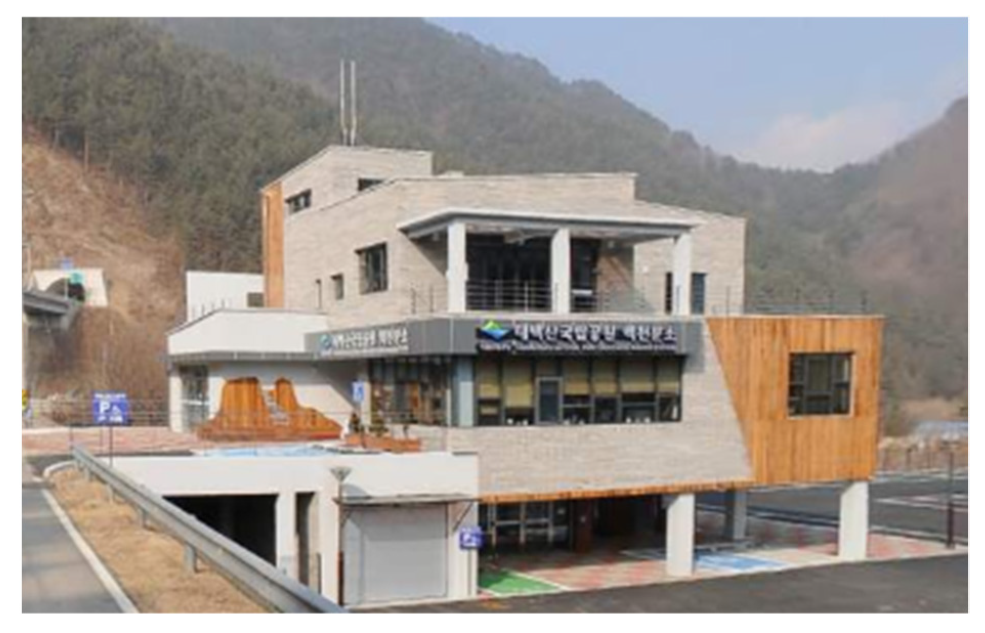
2. Description of Target Building

The information on the target building, a public business facility, is shown in

Table 1. Target building information.

Type	Office
Construction year	2020
Building footprint (m2)	413.35
Gross floor area (m2)	840.98
Building-to-cover ratio	10.33
Floor area ratio	17.18
Height (m)	15
Structure	Reinforced concrete structure
Area and height of each floor	F1	Floor area (m2)	234.34
		Height (m)	4.2
	F2	Floor area (m2)	285.81
		Height (m)	3.85
	F3	Floor area (m2)	166.90
		Height (m)	3.5
	Roof space	Floor area (m2)	23.76
		Height (m)	3.45

, and the picture of the target building is given in Figure 2. The only known information about the target building was the design drawings. Other details such as occupant information and the control algorithm for the cooling and heating system installed in the building were not known. The building energy consumption data for less than one year was insufficient; hence, there was a limit to predicting the energy consumption of the building using only a physical or data-driven model. Consequently, the energy consumption of the building was predicted using a hybrid model.

The U-value and solar heat gain coefficient (SHGC) information on the walls and windows of the target building from the construction drawings are shown in

Table 2. Building envelope properties.

	U-Value (W/m2K)	Solar Heat Gain Coefficient (-)
External wall	0.2733	-
Internal wall	0.2854	-
Ceiling	0.2511	-
Floor	0.2520	-
Windows, curtain wall	1.1000	0.620
Windows at office	0.9000	0.460
Glass doors	1.2600	0.212

. Furthermore, the specifications and installation information on the heat pump from the design and electrical drawings of the cooling and heating equipment are shown in

Table 3. Heat pump specification.

Type	Cooling Capacity (kW)	Cooling COP	Heating Capacity (kW)	Heating COP	Conditioning Area and Number of Units
					Floor	Conditioning Area (m2)	Units
Wall-mounted type	3.2	5.37	3.6	2.82	F1	-	-
					F2	146.94	4
					F3	52.53	2
					Total	199.47	6
Multi type	6	5.7	7.2	3.1	F1	55.11	2
					F2	123.27	4
					F3	-	-
					Total	178.38	6
High-capacity type	11	5	13.2	3	F1	-	-
					F2	-	-
					F3	54.68	1
					Total	54.68	1

COP: Coefficient of performance.

.

A building energy management system (BEMS) was introduced in the target building, which collected the heat pump energy consumption data. The collected heat pump electricity usage data are displayed in Figure 3. After being installed in December 2020, the BEMS underwent a commissioning phase for one month. This study used a total of 5639 heat pump hourly energy consumption measurements from 1 January to 23 August 2021, after the commissioning phase.

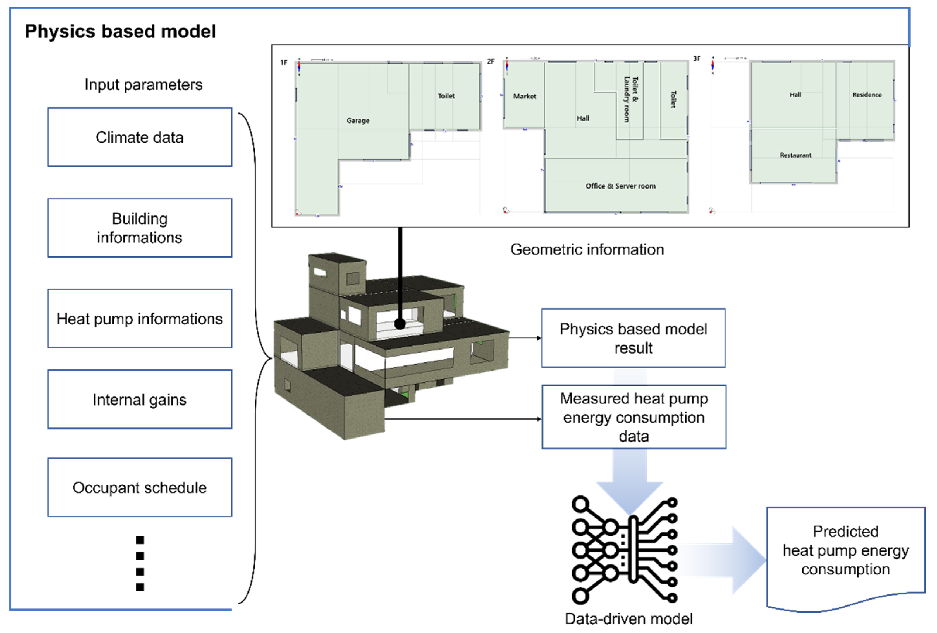
3. Proposed Hybrid Model

3.1. Development of Physical Model of Target Building

The building was modeled using IDA-ICE 4.8 SP2 (EQUA Simulation AB). IDA-ICE is a dynamic building simulation software for the analysis of indoor climate as well as energy consumption. In this study, a physical model of the target building was constructed by using the IDA-ICE built-in tools, and input variables are selected as follows. Table 1 and Table 2 were used for the building shape information, U-values of walls and windows, and SHGC. The capacity and COP input values of the heat pump system were set as in Table 3. The meteorological data consisted of the ambient temperature, relative humidity, cloudiness, wind speed and direction, and total horizontal solar radiation of the target area from 1 January to 23 August 2021, provided by the Korea Meteorological Administration [20]. However, the data provided did not include horizontal solar radiation data; therefore, data measured at nearby observatories were directly separated by the decomposition model proposed by Kasten and Czeplak [21,22] and used as input values.

The assumed occupant schedule followed the ISO office building standard schedule (13790) [23], with the indoor heat gains per unit area and the operation schedule set as the input values as listed in

Table 4. Internal heat gains according to occupant schedules.

Days	Time	Conditioned Zone (W/m2)	Unconditioned Zone (W/m2)
Weekdays	07:00–17:00	20	8
	17:00–23:00	2	1
	23:00–07:00	2	1
Weekend	07:00–17:00	2	1
	17:00–23:00	2	1
	23:00–07:00	2	1

. The indoor temperature was set to 20 °C for heating and 30 °C for cooling, considering that the target building was located in a mountainous area. Furthermore, the opening and closing of windows was controlled according to the room temperature. Reference values were used for the schedule and set temperatures, which could not be verified by field data. Although the target building might have a specific usage pattern different from the assumed settings, automatic fitting was expected to be possible through a data-driven model.

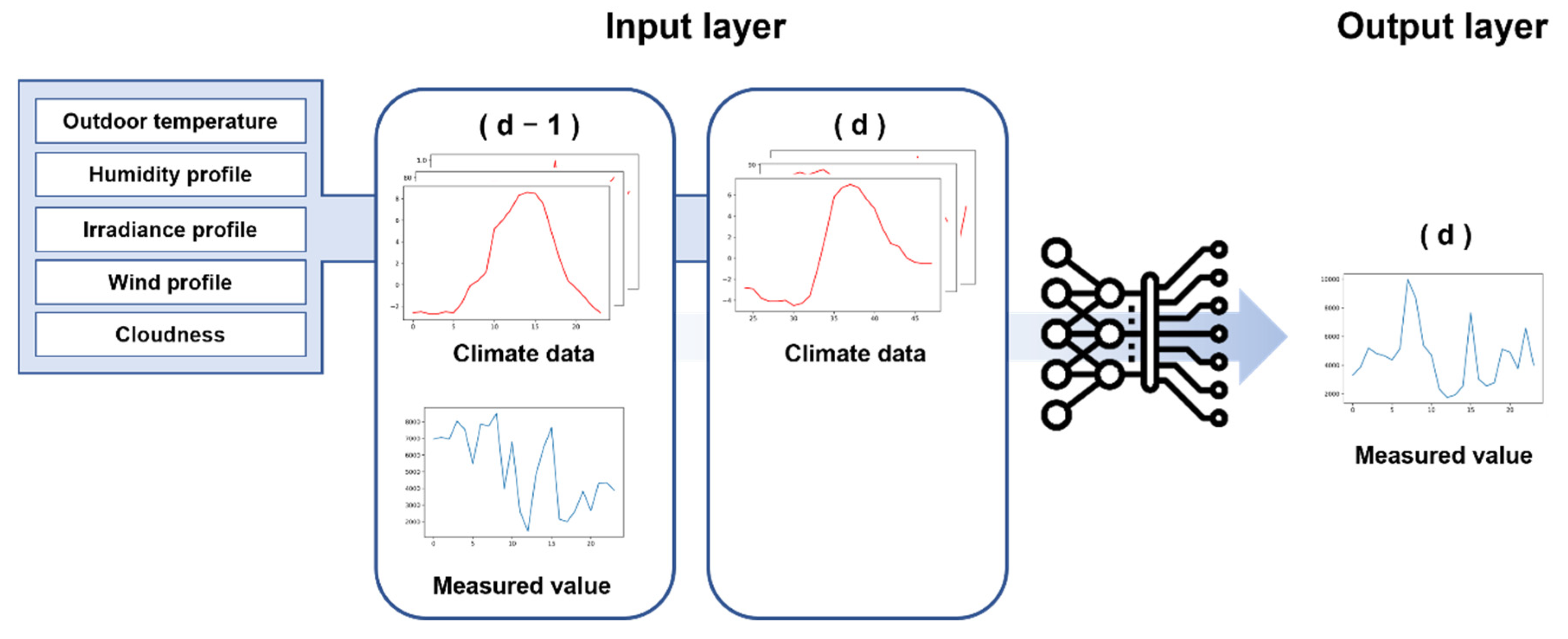
3.2. Reference Data-Driven Model

This section describes a reference data-driven model to evaluate the performance of the proposed hybrid model in this study. A total of 5639 weather data observed from 1 January to 23 August 2021, and heat pump usage data collected from the BEMS during the same period were used as the input data for the model. Each input data had different units, dimensions, and scales; therefore, if the input data were used in the data-driven model without preprocessing, the model result would be biased towards the larger values among the input data, or the model loss could increase and divergence might occur. To minimize these problems, the input data were normalized using the following formula and preprocessed to have values of the same distribution between 0 and 1.

$$x_{std}=\frac{x-\min \left(x\right)}{\max \left(x\right)-\min \left(x\right)}$$

(1)

The long short-term memory (LSTM) model, which is well-suited to time series data prediction, was used as the data-driven model. The LSTM model is an improved model of the recurrent neural network (RNN) model, which is mainly used for sequential data processing. This model solves the problem [24] caused by the loss of past information stored in the hidden layer, as the size of the input data generated in the conventional RNN model increases by installing a gate that shares the cell-state between the LSTM layers. The LSTM model is characterized by higher performance in short-term prediction than that of other data-driven models [25,26,27].

As shown in Figure 4, the input and output layers of the data-driven model were configured using preprocessed data. The input layer of the model was composed of weather data observed one day before (d − 1) the time of prediction, and heat pump usage and weather data observed at the time of prediction (d). Moreover, the output layer of the model was configured so that the model could predict the actual energy consumption of the heat pump at the time of prediction. The input and output data consisted of data measured in units of time as a vector with an interval of one day.

The training and test data of the data-driven model were set as shown in Figure 5, and were distributed by dividing the 5639 data from 1 January to 23 August 2021 into 4 cases. Case 1 predicted the heat pump cooling energy consumption from 17 to 23 August by training the model with data from 1 January to 16 August. Case 2 predicted the heat pump heating energy consumption from 1 to 7 January by training the model with data from 8 January to 23 August. Case 3 predicted the heat pump heating energy consumption from 22 to 28 February by training the model with data from 1 January to 21 February. Lastly, Case 4 predicted the heat pump cooling energy consumption from 17 to 23 August by training the model with data from 26 June to 16 August. Cases 3 and 4 only stored the learning data in the cooling and heating periods.

The LSTM model consisted of a single layer, and the number of epochs was set to 100. The activation function was set as the rectified linear unit (ReLU) [28]. The remaining hyperparameters were set to values calculated using the hyperband optimization algorithm [29]. This algorithm repeats short trainings to find parameter values with high performance and gradually increases the training epochs after setting an arbitrary value as the initial value within the range of the hyperparameter entered as the input value. The hyperband algorithm was implemented using the Tensorflow Keras tuner.

Table 5. Boundary conditions of hyperband optimization algorithm.

	Min	Max	Step
Number of neurons	16	512	16
Learning rate	1 × 10−6	1 × 10−3	-
Batch size	16	64	16
Dropout	0	0.5	0.01

shows the hyperparameter setting range input to the hyperband algorithm, and the results are presented in

Table 6. Selected hyperparameter values by hyperband optimization.

	Case 1	Case 2	Case 3	Case 4
Number of neurons	284	492	325	256
Learning rate	4.1065 × 10−4	4.7858 × 10−3	9.6969 × 10−4	8.9327 × 10−4
Batch size	48	48	32	48
Dropout	0.05	0.05	0	0

.

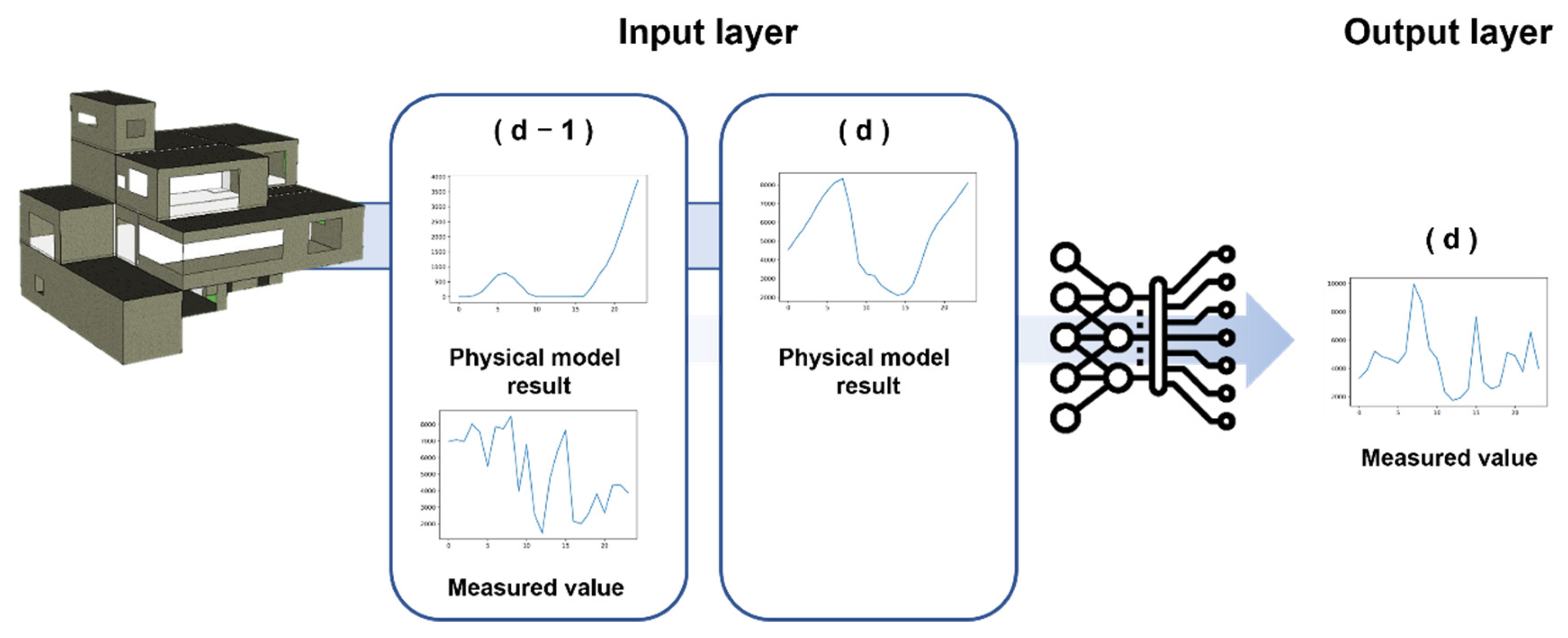
3.3. Hybrid Data-Driven Model Using Physical Model Results as Input Parameters

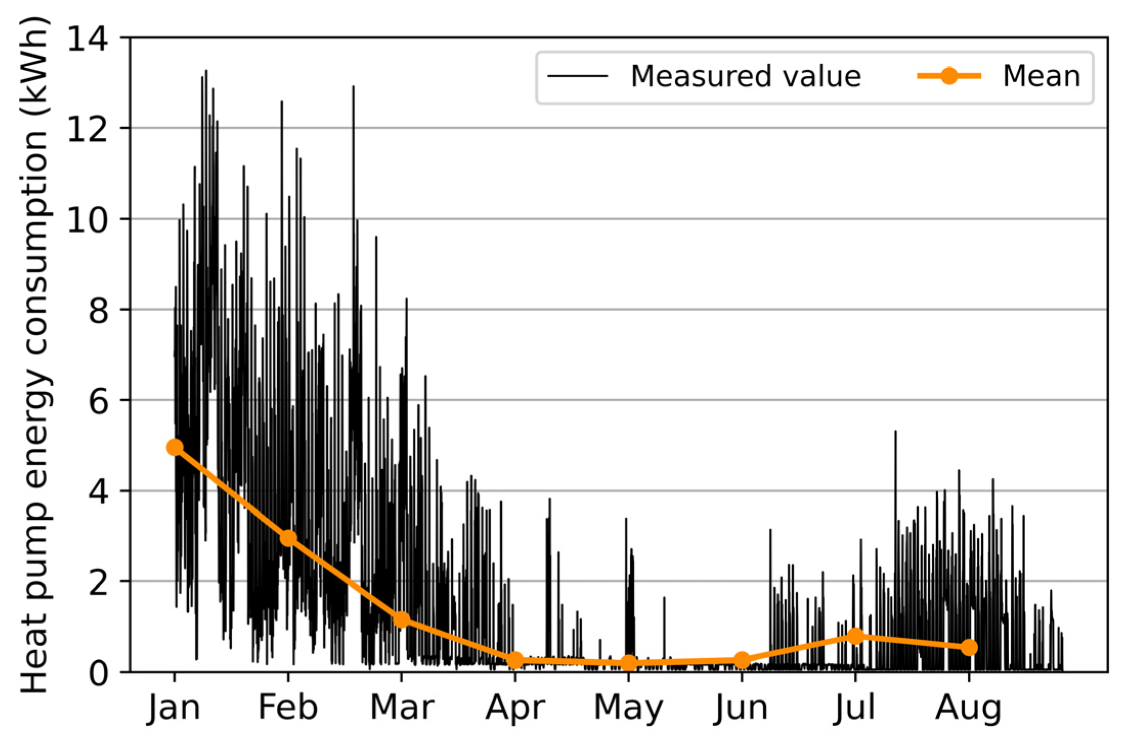
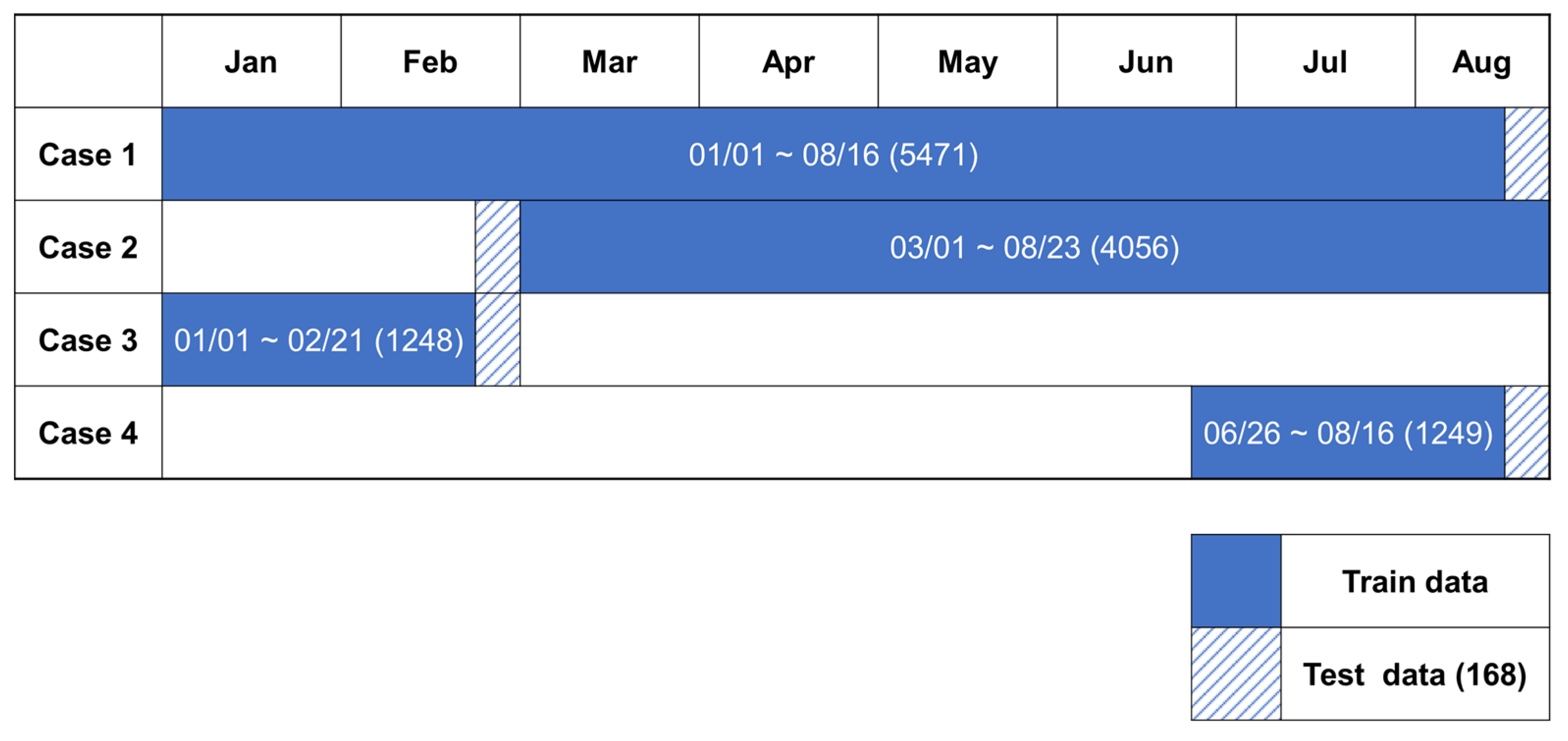
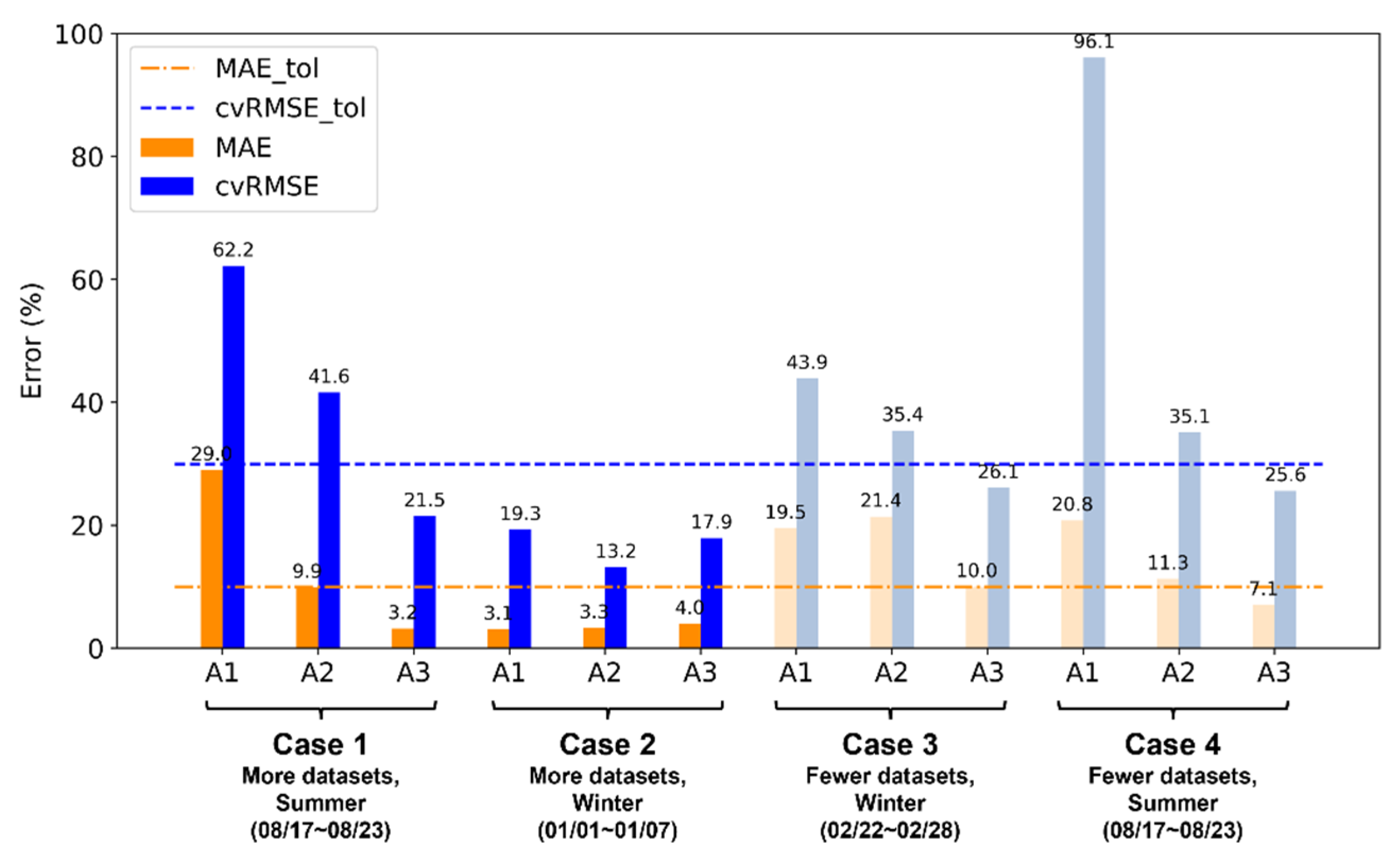
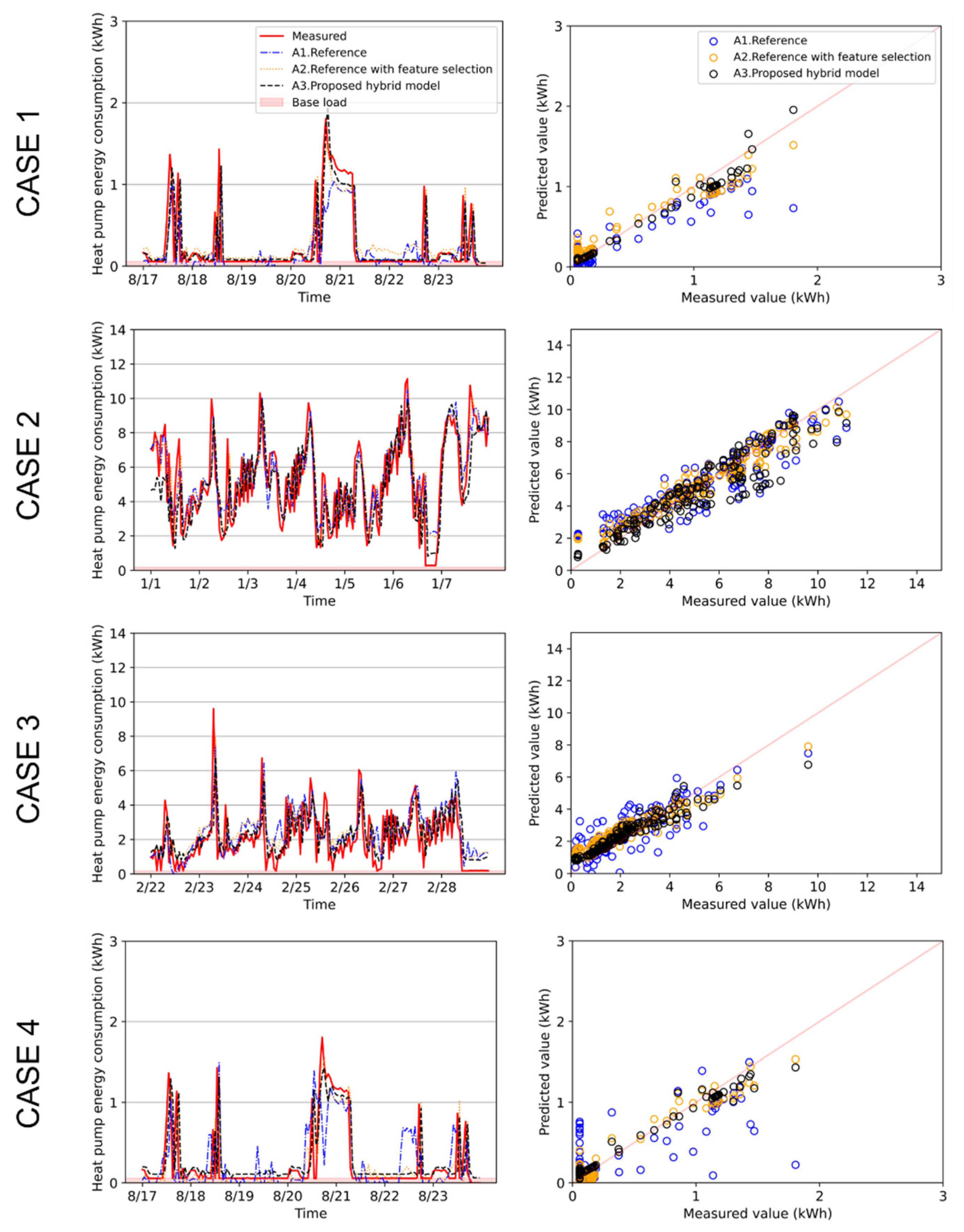
The model proposed in this study was a data-driven model with results of the physical model simulation and the actual heat pump usage as the input data. The compositions of the input and output layers of the data-driven model are shown in Figure 6. The basic model configuration was the same as the data-driven model described in Section 3.2.

The same method was proposed as for the reference data-driven model. In this method, both the physical model and measurement results are used as input values in (d − 1). The model then learns the difference between the two results in the LSTM and predicts the consumption from the physical model result for the next day (d). Differences in the physical boundary conditions such as weather data are reflected in the simulation results. Since similar operating patterns generally occur in office buildings, the data-driven model reflected the difference between the set and actual operation schedules to improve the accuracy. This study verified the model performance by using the weather measured data of the next day under the assumption that the weather forecast was correct. A recent research study on weather forecasting has excellent results, and the forecasting is therefore not expected to have large errors [30].

4. Results

The physical, reference data-driven, and hybrid models proposed in this study were simulated during the data availability period. Furthermore, the coefficient of variation of the root mean square error (cvRMSE) and the mean absolute error (MAE) of the model results and actual heat pump energy consumption data were calculated. The calculation results were checked against the tolerances of ASHRAE Guideline 14: under 30% for cvRMSE and under 10% for MAE [31]. The calculation formulas for cvRMSE and MAE are Equations (2) and (3), respectively. The heating base-load energy consumption was set to 0.183 kWh or less, which was obtained by the electricity consumption most frequently measured from 1 January to 28 February. Similarly, the cooling base-load energy consumption was set to 0.058 kWh or less, obtained by data analysis from 26 June to 23 August.

$$\mathrm{cvRMSE}=\frac{\sqrt{\frac{1}{T}{{\displaystyle \sum }}_{\mathrm{t}=1}^T{\left(E_{\mathrm{meas},\mathrm{t}}-E_{\mathrm{pred},\mathrm{t}}\right)}^2}}{\frac{1}{T}{{\displaystyle \sum }}_{\mathrm{t}=1}^T{E}_{\mathrm{meas},\mathrm{t}}}$$

(2)

$$\mathrm{MAE}=\frac{{{\displaystyle \sum }}_{t=1}^T\left|E_{\mathrm{meas},\mathrm{t}}-E_{\mathrm{pred},\mathrm{t}}\right|}{{{\displaystyle \sum }}_{\mathrm{t}=1}^T{E}_{\mathrm{meas},\mathrm{t}}}$$

(3)

where T is the total actual period of use of the heat pump excluding the period of base-load energy consumption, E is the energy consumption, subscript “meas” is the actual value, and subscript “pred” is the predicted heat pump consumption derived using the model.

Figure 7 shows a comparison of the calculated values using only the physical model and the measured values. The cvRMSE of the results predicted using the physical model was 186% and the MAE was 99%, which does not satisfy the tolerances of the ASHRAE Guideline. Therefore, there is a limit to using the model for the purpose of predicting the energy consumption of a target building. In particular, a large difference in energy consumption occurred in the summer, which is presumed to be due to the cooling being rarely operated due to natural ventilation. In other words, there was a difference in the schedule set for the physical model. These differences in operating patterns may be fitted through a hybrid model; however, there is a risk of lowering the model performance when a result calculated using the physical model is used as an input value for the data-driven model. Therefore, it is necessary to determine whether a result calculated by the physical model is an appropriate input value. Guyon and Elisseeff [32] argued that when the correlation coefficient between the dependent and independent variables is large when selecting the input data of the data-driven model, it is suitable to use the variables as the input data. The calculated correlation coefficient $\rho$ between the physical model results and the measured data using Equation (4) was 0.63, suggesting that it is suitable to use the physical model results as input data for the data-driven model.

$$\rho =\frac{\mathrm{cov}(P,E_{\mathrm{meas}})}{{\sigma }_P{\sigma }_{E_{\mathrm{meas}}}}$$

(4)

where “cov” is the covariance between the two results, σ is the standard deviation, and P is the input variable. E_meas is the measured energy consumption of the heat pump, which was used as the output variable in the data-driven model.

Detailed information such as the occupancy schedule and indoor environment of the target building could not be confirmed. Therefore, the result of using only meteorological data as input data for the data-driven model showed that the error in the prediction of heating energy consumption was smaller than that of the prediction of heat pump cooling energy consumption as seen in Cases 3 and 4 of Reference A1 in

Table 7. Model comparison for prediction accuracy by case.

	Reference (A1)		Reference with Feature Selection (A2)		Proposed Hybrid Model (A3)
	cvRMSE (%)	MAE (%)	cvRMSE (%)	MAE (%)	cvRMSE (%)	MAE (%)
Case 1	62.2	29.0	41.6	9.9	21.5	3.2
Case 2	19.3	3.1	13.2	3.3	17.9	4.0
Case 3	43.9	19.5	35.4	21.4	26.1	10.0
Case 4	96.1	20.8	35.1	11.3	25.6	7.1

Case 1: more datasets, summer (17–23 August), Case 2: more datasets, winter (1–7 January), Case 3: fewer datasets, winter (22–28 February), Case 4: fewer datasets, summer (17–23 August).

. Cases 1 and 2 with a large number of training data showed higher prediction performance than Cases 3 and 4, which were predicted for a similar period. However, the cvRMSE and MAE did not satisfy the tolerance suggested in ASHRAE Guideline 14 in any case except Case 2.

The model prediction performance was not considered good due to the low correlation between the meteorological data elements used as the input variables and the heat pump energy consumption. Therefore, the correlation coefficient of each input data element with the heat pump energy consumption was calculated as listed in

Table 8. Correlation coefficient of each input parameter with the output of the data-driven model.

Parameter	ρ (−)
Outdoor temperature	0.63
Relative humidity	0.23
Wind velocity	0.078
Wind direction	0.067
Diffuse irradiance	0.028
Direct normal irradiance	0.012
Cloudiness	0.0064

. The outdoor air temperature, relative humidity, wind speed, wind direction, diffuse radiation, and direct solar radiation showed close correlations with the heat pump energy consumption, from large to small. The outdoor temperature, which showed the greatest correlation, was similar to the correlation coefficient value obtained between the physical model result and the measured data. Thus, the prediction results were confirmed (center column A2 of Table 7) after a data-driven model was constructed using only the outside temperature as the input data. The model prediction performance was improved compared to that of the data-driven model using all weather data as input data. Case 2 showed excellent prediction performance, satisfying ASHRAE Guideline 14. However, there was a limit to the practical application of the other cases because their results were too far from the allowable error range.

Lastly, the calculation results of the data-driven model using the physical model results as the input data (A3 column of Table 7) satisfied the ASHRAE Guideline 14 tolerance criterion in all cases regardless of the number of training data. Compared with the results of the data-driven model using only the outside temperature as input data, the hybrid model results were better in all cases except Case 2, even though the correlation coefficients between the input and output variables were similar. Here, Case 2 has abundant training data, and its target prediction is on a winter period when a strong correlation is found between energy consumption and weather parameters. Therefore, all the results were within an acceptable range regardless of the input variables and methods.

Figure 8 shows the results according to the data size of the model used for training. MAE_tol and cvRMSE_tol refer to the MAE and cvRMSE tolerance criteria suggested in the ASHRAE Guideline 14, respectively. As in Cases 1 and 2, the more data used for learning, the smaller the input value, and the fewer the errors. Importantly, for the same correlation, the physical model showed the smallest error in general because it directly depicts the change in energy consumption according to the weather change. Finally, Figure 9 shows the predicted hourly energy consumption by cases and models. All the models follow the dynamics of the energy consumption measured at the site. As discussed above, the proposed hybrid model shows superior performance particularly for cases of data scarcity.

In particular, the prediction performance initially shown with the physical model could be dramatically improved by using the hybrid model for the summer period (compare Figure 7) when a large error is found for the physical model. Figure 10 shows the accuracy improvement when the proposed hybrid model predicts the summer energy consumption. Here, it is worthwhile noting that the proposed model has input vectors obtained from the physical model. The physical model responds to the weather changes under its thermal characteristics while the data-driven part of the proposed hybrid model may compensate for the error between physical model results and measured values by adjusting weight factors to reduce the uncertainty of the energy consumption pattern of occupants, heat pump operation schedules, set point temperatures, and so on.

5. Conclusions

In this study, we predicted a building’s energy consumption by using the results of a physical model as the input data for a data-driven model where there was insufficient information about the target building or historical building energy consumption data. Furthermore, the model’s results were compared with the predicted results using the physics-based and data-driven models alone.

The cvRMSE and MAE of the results were 186% and 99%, respectively, calculated from the physical model and heat pump energy consumption of the target building. Thus, there was a limit to expressing the energy consumption of the target building using only the physical model. However, the correlation coefficient between the results calculated from the physical model and the heat pump consumption of the target building was 0.63, indicating a linear relationship. Therefore, it was considered appropriate to use the physical model results as the input data of the data-driven model.

The prediction results for the building’s energy consumption estimated by constructing a data-driven model using meteorological data as input data were not appropriate. The prediction performance was assumed to decrease due to the low correlation coefficient between the input variables and the measured heat pump energy consumption. Therefore, feature selection was performed by analyzing the correlation between the meteorological data elements used as input data and the building’s energy consumption.

As a result of the feature selection, the correlation coefficient between the outdoor temperature and the measured heat pump energy consumption was 0.63. This was similar to the correlation coefficient between the physical model results and the measured heat pump energy consumption. After constructing a data-driven model using only outdoor temperature as an input value, the model showed better prediction performance.

Finally, when the prediction was performed using the data-driven model with the physical model results as input data, the results of this proposed hybrid model satisfied the criteria of ASHRAE Guideline 14, regardless of the number of training data.

To the authors’ knowledge, the data scarcity issue is more important in the engineering field as data are target object dependent and public data cannot be easily reused. This preliminary study on physics-based data-driven modeling can be a solution for various prediction applications.

References

1. IEA. Tracking Buildings 2021; IEA: Paris, France, 2021; Available online: https://www.iea.org/reports/tracking-buildings-2021 (accessed on 22 March 2022).
2. González-Torres, M.; Pérez-Lombard, L.; Coronel, J.F.; Maestre, I.R.; Yan, D. A review on buildings energy information: Trends, end-uses, fuels and drivers. Energy Rep. 2022, 8, 626–637. [Google Scholar] [CrossRef]
3. IEA. IEA World Energy Balances 2021; IEA: Paris, France, 2021; Available online: https://www.iea.org/data-and-statistics/data-product/world-energy-statistics-and-balances (accessed on 22 March 2022).
4. Fumo, N. A review on the basics of building energy estimation. Renew. Sustain. Energy Rev. 2014, 31, 53–60. [Google Scholar] [CrossRef]
5. Li, C.Z.; Zhang, L.; Liang, X.; Xiao, B.; Tam VW, Y.; Lai, X.; Chen, Z. Advances in the research of building energy saving. Energy Build. 2021, 254, 111556. [Google Scholar] [CrossRef]
6. Liu, S.; Zou, Y.; Ji, W.; Zhang, Q.; Ahmed, A.; Han, X.; Shen, Y.; Zhang, S. Energy-saving potential prediction models for large-scale building: A state-of-the-art review. Renew. Sustain. Energy Rev. 2022, 156, 111992. [Google Scholar] [CrossRef]
7. Bünning, F. Marrying Machine Learning and Model Predictive Control for efficient Building Energy Management. Ph.D. Thesis, ETH Zurich, 2021. Available online: https://www.research-collection.ethz.ch/handle/20.500.11850/526883 (accessed on 22 March 2022).
8. Deb, C.; Dai, Z.; Schlueter, A. A machine learning-based framework for cost-optimal building retrofit. Appl. Energy 2021, 294, 116990. [Google Scholar] [CrossRef]
9. Chen, Y.; Guo, M.; Chen, Z.; Chen, Z.; Ji, Y. Physical energy and data-driven models in building energy prediction: A review. Energy Rep. 2022, 8, 2656–2671. [Google Scholar] [CrossRef]
10. Al-Hyari, L.; Kassai, M. Development of TRNSYS model for energy performance simulation of variable refrigerant flow air-conditioning system combined with energy recovery ventilation. Int. J. Green Energy 2021, 18, 390–401. [Google Scholar] [CrossRef]
11. Im, P.; Joe, J.; Bae, Y.; New, J.R. Empirical validation of building energy modeling for multi-zones commercial buildings in cooling season. Appl. Energy 2020, 261, 114374. [Google Scholar] [CrossRef]
12. Chen, Y.; Chen, Z.; Xu, P.; Li, W.; Sha, H.; Yang, Z.; Li, G.; Hu, C. Quantification of electricity flexibility in demand response: Office building case study. Energy 2019, 188, 116054. [Google Scholar] [CrossRef]
13. Soleimani-Mohseni, M.; Nair, G.; Hasselrot, R. Energy simulation for a high-rise building using IDA ICE: Investigations in different climates. Build. Simul. 2016, 9, 629–640. [Google Scholar] [CrossRef]
14. Sun, Y.; Haghighat, F.; Fung, B.C.M. A review of the-state-of-the-art in data-driven approaches for building energy prediction. Energy Build. 2020, 221, 110022. [Google Scholar] [CrossRef]
15. An, D.; Kim, N.H.; Choi, J.H. Practical options for selecting data-driven or physics-based prognostics algorithms with reviews. Reliab. Eng. Syst. Saf. 2015, 133, 223–236. [Google Scholar] [CrossRef]
16. Dong, B.; Li, Z.; Rahman, S.M.M.; Vega, R. A hybrid model approach for forecasting future residential electricity consumption. Energy Build. 2016, 117, 341–351. [Google Scholar] [CrossRef]
17. Amasyali, K.; El-Gohary, N. Hybrid approach for energy consumption prediction: Coupling data-driven and physical approaches. Energy Build. 2022, 259, 111758. [Google Scholar] [CrossRef]
18. Xu, X.; Taylor, J.E.; Pisello, A.L.; Culligan, P.J. The impact of place-based affiliation networks on energy conservation: An holistic model that integrates the influence of buildings, residents and the neighborhood context. Energy Build. 2012, 55, 637–646. [Google Scholar] [CrossRef]
19. Li, A.; Xiao, F.; Fan, C.; Hu, M. Development of an ANN-based building energy model for information-poor buildings using transfer learning. Build. Simul. 2021, 14, 89–101. [Google Scholar] [CrossRef]
20. Korea Meteorological Administration. Available online: https://www.weather.go.kr/ (accessed on 15 October 2021).
21. Martin, M.; Berdahl, P. Characteristics of infrared sky radiation in the United States. Sol. Energy 1984, 33, 321–336. [Google Scholar] [CrossRef] [Green Version]
22. Kasten, F.; Czeplak, G. Solar and terrestrial radiation dependent on the amount and type of cloud. Sol. Energy 1980, 24, 177–189. [Google Scholar] [CrossRef]
23. ISO 13790; Energy Performance of Buildings-Calculation of Energy Use for Space Heating and Cooling. 2008. Available online: https://www.iso.org/obp/ui/#iso:std:iso:13790:ed-2:v1:en (accessed on 22 March 2022).
24. Cortez, B.; Carrera, B.; Kim, Y.J.; Jung, J.Y. An architecture for emergency event prediction using LSTM recurrent neural networks. Expert Syst. Appl. 2018, 97, 315–324. [Google Scholar] [CrossRef]
25. Wang, Z.; Hong, T.; Piette, M.A. Building thermal load prediction through shallow machine learning and deep learning. Appl. Energy 2020, 263, 114683. [Google Scholar] [CrossRef] [Green Version]
26. Siami-Namini, S.; Tavakoli, N.; Namin, A.S. A comparison of ARIMA and LSTM in forecasting time series. In Proceedings of the 2018 17th IEEE International Conference on Machine Learning and Applications (ICMLA), Orlando, FL, USA, 17–20 December 2018; pp. 1394–1401. [Google Scholar] [CrossRef]
27. Di Natale, L.; Svetozarevic, B.; Heer, P.; Jones, C.N. Physically Consistent Neural Networks for building thermal modeling: Theory and analysis. arXiv 2021, arXiv:2112.03212. [Google Scholar]
28. Ramachandran, P.; Zoph, B.; Le, Q.V. Searching for activation functions. arXiv 2017, arXiv: 1710.05941. [Google Scholar] [CrossRef]
29. Li, L.; Jamieson, K.; DeSalvo, G.; Rostamizadeh, A.; Talwalkar, A. Hyperband: A novel bandit-based approach to hyperparameter optimization. J. Mach. Learn. Res. 2017, 18, 6765–6816. [Google Scholar]
30. Jeon, B.K.; Kim, E.J. Next-day prediction of hourly solar irradiance using local weather forecasts and LSTM trained with non-local data. Energies 2020, 13, 5258. [Google Scholar] [CrossRef]
31. American Society of Heating, Ventilating, and Air Conditioning Engineers (ASHRAE). Errata Sheet for ASHRAE Guideline 14-2002, Measurement of Energy and Demand Savings; American Society of Heating, Ventilating, and Air Conditioning Engineers: Atlanta, GA, USA, 2008. [Google Scholar]
32. Guyon, I.; Elisseeff, A. An introduction to variable and feature selection. J. Mach. Learn. Res. 2003, 3, 1157–1182. [Google Scholar]
Figure 1. Proposed hybrid model with a physics-based model.
Sustainability 14 09464 g001
Figure 2. Target building.
Sustainability 14 09464 g002
Figure 3. Heat pump energy consumption data collected from building energy management system.
Sustainability 14 09464 g003
Figure 4. Input and output layers of the reference model, where d is the time of prediction.
Sustainability 14 09464 g004
Figure 5. Cases with different training and test data sets.
Sustainability 14 09464 g005
Figure 6. Input and output layers of proposed hybrid model.
Sustainability 14 09464 g006
Figure 7. Simulation results of physical model.
Sustainability 14 09464 g007
Figure 8. Comparison of prediction error for each case.
Sustainability 14 09464 g008
Figure 9. Prediction results for each case.
Sustainability 14 09464 g009
Figure 10. Comparison of physical model results with the results of the proposed model trained with Case 4 data (summer period).
Sustainability 14 09464 g010