Carbon Emissions, Economic Growth, Urbanization, and Foreign Trade in China: Empirical Evidence from ARDL Models

Abstract

Based on the autoregressive distribution lag (ARDL) model, this paper conducts an empirical study on the relationship between carbon emissions, economic growth, urbanization, and foreign trade in China from 1971 to 2020. The results show that when carbon emissions, economic growth, and urbanization are used as explained variables, there is a long-term cointegration relationship with other variables. In the long-term relationship, urbanization has a significant positive effect on economic growth and carbon emissions, with coefficients of 2.2172 and 0.2921, respectively. The long-term elasticity coefficient of economic growth to urbanization is 0.4864, passing the 1% significance test. In the short-term relationship, economic growth and carbon emissions, urbanization and carbon emissions, and economic growth and urbanization are all mutually reinforcing relationships, and foreign trade will suppress carbon emissions in the short term. Therefore, policymakers should transform the urbanization model and develop a green economy to achieve environmental sustainability.

1. Introduction

Environmental quality has become one of the obstacles to the sustainable development of countries in the world. There is no doubt that rapid economic growth and urbanization have exacerbated environmental pollution [1]. The signing of the Paris Agreement in 2015 has become a symbol of controlling global environmental deterioration, and the agreement has proposed long-term and short-term goals for temperature changes [2]. With the rapid development of economic growth and urbanization, economic and social activities have continuously increased, resulting in a large amount of energy consumption and carbon emissions. Therefore, how to control carbon emissions in the process of economic growth has become an urgent problem for governments of all countries, especially developing countries [3].

The relationship between variables such as carbon emissions, economic growth, urbanization, and foreign trade has attracted the attention of many researchers because of its global significance. Researchers work to investigate whether carbon emissions are the result of economic growth, urbanization, foreign trade, or just a stand-alone environmental issue [4]. Economies around the world rely on fossil energy consumption for high economic growth to handle the demands of growing populations [5]. Hence, economic growth is one of the main factors leading to carbon emissions [6]. Grossman and Krueger pointed out that the initial stage of economic growth will bring about environmental pollution, and when economic growth reaches a certain level, environmental pollution will gradually decrease, which is the Environmental Kuznets Curve (EKC) hypothesis [7,8]. However, the current economic development of most countries or regions requires more nonrenewable energy, which pollutes the environment [9], especially for developing countries. Economic growth requires more output, and energy consumption must meet the greatest amount of economic activity and human needs, leading to more pollution and waste, while putting pressure on the environment and natural resources. According to the World Bank report, from 1990 to 2021, the total world GDP rose from 22.78 trillion to 96.1 trillion. From 1990 to 2019, carbon dioxide emissions increased from 20,625,273 kg to 34,344,006 kg. Yin et al. [10] said economic growth caused some environmental problems and found a positive relationship between economic growth and carbon emissions. In addition, some studies have investigated the relationship between economic growth and carbon emissions in different regions, such as Iran [11], China [12], and BRICS economies [13]. These confirm that economic growth is a key factor affecting carbon emissions.

After the Industrial Revolution, urbanization has made great strides around the world. In the process of urbanization, urban areas and populations have increased, and the construction of infrastructure and housing has generated significant energy consumption. In addition, rising material conditions have raised the standard of living, leading to greater living energy consumption [14,15]. However, energy consumption was considered a major contributor in increased carbon emissions, particularly for non-fossil-fuel use. In addition, Urbanization releases economic demand and boosts economic growth. In turn, energy consumption, an integral factor in the economic growth process, provides production or transport activities for economic growth, which will further increase carbon emissions [16,17]. The economic level, geographical location, climatic conditions, topography, and altitude of the study area cause significant differences in the rate, quality, and carbon emissions of urbanization [18]. Therefore, many researchers have investigated the relationship between urbanization and carbon emissions in various regions of the world, such as China [19], Indonesia [20], the United States [21], and Singapore [22]. The findings indicated that there was no standardized relationship between urbanization and carbon emissions and that the relationship was either positive, negative, inverted U-shaped, or absent. Thus, the multiple relationships between urbanization and carbon emissions are complex and need further exploration.

Many studies showed that foreign trade boosted economic development and reduced poverty [23]. Foreign trade drives economic growth through the diffusion of knowledge and technological progress, boosting competition in domestic and international markets, and thus, optimizing production processes [24]. In addition, the relationship between carbon emissions and foreign trade is called the environmental pollution paradise hypothesis. Specifically, developed countries have transferred technologies that lead to rising carbon emissions to developing countries in the form of foreign trade and investment [25]. Some studies have confirmed a positive relationship between foreign trade and carbon emissions. Further, with the growth of imports and exports, carbon emissions show an increasing trend [26,27].

Thus, a strong relationship exists between carbon emissions, economic growth, urbanization, and foreign trade. Empirical research on the relationship between macroeconomic variables and the environment is essential in resolving the debate on sustainable development and environmental degradation. Nevertheless, the characteristics and economic levels are different in each country or region; so, the conclusions are not universal.

In recent decades, China′s economic scale has been expanding, and its degree of openness has been increasing. At the same time, China has experienced the largest urbanization in human history. Due to the increase in economic and social activities, China′s carbon emissions are increasing rapidly, gradually becoming the most carbon-emitting country in the world and causing damage to the ecological environment [28], and the share of carbon emissions accounts for 28.8% of the world. The Chinese government is under enormous pressure from the international community on the issue of carbon emissions. As an important vehicle for global economic development, China needs to alleviate the dual pressures of the international community and the structural transformation of its domestic economy. The Chinese government is under enormous pressure from the international community on the issue of carbon emissions. As an important vehicle for global economic development, China needs to alleviate the dual pressures of the international community and the structural transformation of its domestic economy. Therefore, how to realize the coordinated development of carbon emission, economic growth, urbanization, and foreign trade has become an urgent problem for China.

To achieve sustainable development goals, the Chinese government has formulated a series of carbon emission reduction policies and measures. The Chinese government announced at the 2020 Climate Ambition Summit that it is striving to peak CO₂ emissions by 2030 and is working towards achieving carbon neutrality by 2060. By 2030, China′s CO₂ emissions per unit of GDP will drop by more than 65% compared with 2005, and the share of nonfossil energy in primary energy consumption will reach around 25% [29]. Therefore, there is a focus on the causes of carbon emissions. Exploring the long-term and short-term dynamic relationship between carbon emissions, economic growth, urbanization, and foreign trade is greatly significant for achieving sustainable development.

Scholars have contributed extensively to studies on the long-term and short-term relationships between carbon emissions, economic growth, urbanization, and foreign trade. Their research has a powerful reference value and provides a solid basis for further research, but the following issues still need to be addressed: (1) Existing studies mainly focus on the relationship between two variables or three variables. Few studies take China as the research object and study carbon emissions, economic growth, urbanization, and foreign trade under the same framework. (2) Whether there is a long-term relationship between China’s carbon emissions, economic growth, urbanization, and foreign trade. Whether economic growth, urbanization, and foreign trade will inhibit carbon emissions; whether carbon emissions, urbanization, and foreign trade will promote economic growth; and how carbon emissions, economic growth, and foreign trade will affect urbanization are issues worth pondering and exploring. Further, it is of great significance for China to achieve sustainable development and to provide a reference for other countries or regions. Due to this, this paper selects China’s panel data from 1971 to 2020; uses the ARDL model to conduct empirical research on the relationship between carbon emissions, economic growth, urbanization, and foreign trade; and explores the long-term and short-term dynamic relationship between the four.

The rest of the study is prepared as follows. The “Literature review” section describes the literature review, and the “Data and methodology” section reports the model and methods. The “Empirical and discussion” section gives the empirical results. The “Conclusion and policy implications” section shows the conclusions and policy.

2. Literature Review

The industrial economy has replaced the traditional agricultural economy, increasing productivity and accelerating economic growth. At the same time, there has been an increased demand for labor in the rapidly growing urban centers, which led to rural–urban migration and accelerated urbanization. In addition, most countries attracted external investment to expand their foreign trade in pursuit of higher economic growth. After tasting the sweet fruits of economic growth, people blindly pursued economic growth and neglected the problem of environmental pollution. Therefore, we cannot help but wonder whether economic growth, urbanization, and foreign trade will further aggravate environmental pollution. Conversely, what about the impact of environmental pollution on economic growth, urbanization, and foreign trade.

The first empirical study to investigate the link between economic growth and environmental degradation (particularly CO₂ emissions) was the paper by Kraft and Kraft [30], which used data from 1947 to 1974 for the United States and found evidence of Granger causality from output to energy consumption. Later, some scholars selected panel data from different countries or regions to study the relationship between variables related to environmental pollution, the most representative of which is EKC. Ganda et al. [31] and Pata [32] took South Africa and Turkey as research objects and verified the EKC relationship between energy consumption, economic growth, and carbon emissions. Yao et al. [33] used the modified ordinary least squares method and dynamic ordinary least squares method to study the relationship between energy structure, carbon emission, and economic growth in 17 developing countries, and the results showed an EKC relationship between economic growth and renewable energy. However, Dogan and Turkekul [21] used the per-capita GDP, carbon emissions, trade openness, urbanization, and financial openness of the United States as variables to find the EKC relationship between the variables but did not find evidence of the existence of an EKC curve between the variables. Kaika and Zervas [34] proposed that most studies attempt to examine the EKC curve between environmental degradation and related factors (such as income, international trade, energy efficiency, and economic growth). Most studies show that economic growth does not reduce carbon emissions over time and pointed out that carbon emissions are related to economic growth through energy consumption.

Some scholars use econometric models to explore the long-term and short-term dynamic relationship between variables such as carbon emissions, economic growth, urbanization, and foreign trade, to provide a reference for the sustainable development of a region or country. Lee and Yoo [35], Dimitriadis et al. [36], and Wang and Li [37] selected panel data from Mexico, 68 developing countries, and 29 provinces in China to discuss the long-term and short-term relationship between carbon emissions, economic growth, energy consumption, and urbanization. Zhang et al. [38] and Yang [39] studied the EKC relationship among carbon emissions, urbanization, economic growth, and trade openness by using a fixed (random) effect model and autovector regression model with countries along the “Belt and Road” and China, respectively. They uncovered strong evidence for the existence of an EKC curve between economic growth, urbanization, and carbon emissions. Most of the above studies use cointegration and error correction models to explore long-term and short-term relationships between variables. However, the cointegration and error correction models have high requirements on the number of samples. Smaller sample size may reduce the accuracy of the model and, to some extent, limit the scope of its application.

In recent years, the ARDL model has gradually emerged. This model has low requirements on the number of samples, is suitable for small sample research, and has high model stability. It is widely used in research in various fields. Qayyum et al. [40] used the ARDL model to analyze the relationship between air PM2.5 content and the number of respiratory tract patients. Attiaoui and Boufateh [41] used ARDL to study the impact of climate change on crops. Malik et al. [42] used this model to explore the relationship between oil price, foreign investment, and economic growth. The ARDL model has an extensive range of applications. It can not only analyze the long-term and short-term relationship between variables but also predict the changing trend of variables. For example, Adom and Bekoe [43] predicted the overall electricity consumption in Ghana. Shen et al. [44] combined the Granger causality test to predict the electricity consumption of China′s energy-intensive industries.

As the ARDL model has achieved important results in other related fields, many scholars have introduced it into the study of environmental economics to study the long-term and short-term relationships between related variables. Bosah et al. [45] analyzed the panel data on energy consumption, economic growth, urbanization, and carbon emissions in 15 countries. The results show that urbanization has no significant impact on environmental quality, and energy consumption will cause damage to the environment in the long and short term. Ali et al. [22] and Pata [32], respectively, analyzed the relationship between urbanization and carbon emissions in Singapore and Turkey, but the two obtained different research results; urbanization in Singapore inhibits carbon emissions, while urbanization in Turkey promotes carbon emissions. Ahmed et al. [28] analyzed the impact of globalization, economic growth, and financial development on carbon footprint with Japanese research subjects. The results showed that energy consumption and financial development would significantly increase carbon footprint, while the relationship between economy and carbon footprint showed an inverted U shape, confirming that EKC assumes validity in Japan. Wen and Dai [46] conducted an empirical study on China′s trade openness, environmental regulation, and human capital. The development of environmental regulation and trade openness has a significant positive effect on human capital.

Reviewing the above literature, we find that the ARDL model has been used extensively in environmental economics. It is mainly concerned with the study of long-term and short-term relationships between variables such as urbanization, industrialization, economic growth, carbon emissions, energy consumption, financial development, and trade openness. It is worth noting that even when the relationship between the same variables is studied, the findings may be inconsistent. Some of the findings are not generalizable because of differences in the study sample due to different study regions, periods, and indicators. In addition, variable data series over time may also be another source of inconsistent findings. Therefore, regular studies of the relationships between the various variables are needed to explore the actual impacts between the variables.

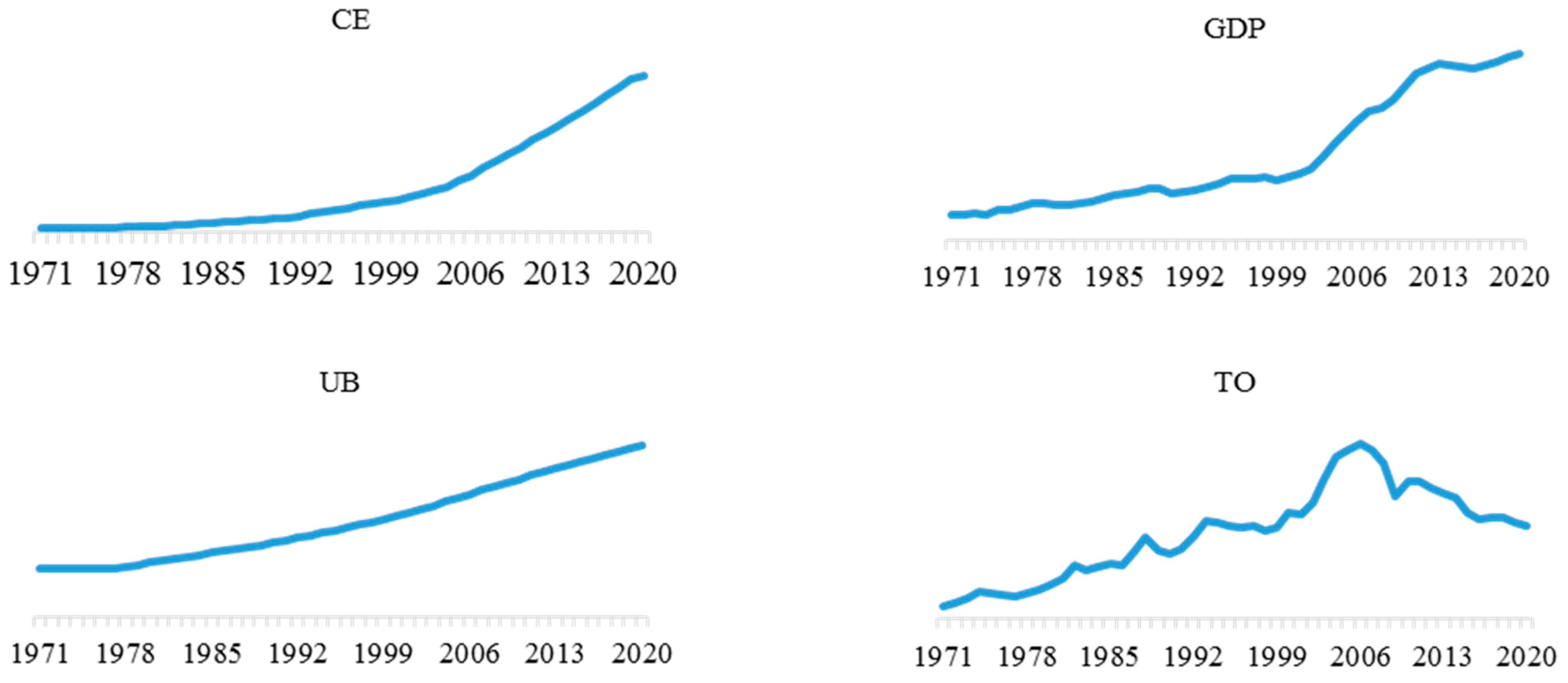
This study takes China as an example, selects time series data from 1971 to 2020, and applies the ARDL estimation method to explore the interaction between carbon emissions, economic growth, urbanization, and foreign trade. We take carbon emissions, economic growth, urbanization, and foreign trade as explained variables to explore the long-term and short-term relationships with other remaining variables. In addition, the study will provide helpful policy insights for other developing countries in the same situation.

3. Data and Methodology

3.1. Variables and Data

We deeply study the long-term and short-term dynamics of China’s carbon emissions, economic growth, urbanization, and foreign trade, using the following indicators as variables (shown in

Table 1. Variable description.

Variable	Variable Description	Unit	Source
Carbon emissions	Per capita carbon emissions (CE)	Tce	World bank
Economic growth	Per capita GDP (GDP)	Yuan	World bank
Urbanization	Urbanization rate (UB)	%	World bank
Foreign trade	Trade as a percentage of gross national product (TO)	%	World bank

).

We used time series data from 1960 to 2020 in China. However, the actual estimates are based on data from 1971–2020, as foreign trade data are only available before 1971. All variables are converted into natural logarithm form for consistent and robust estimates; specifically, they are represented by $LnC{E}_t$, $LnGD{P}_t$, $LnU{B}_t$, $LnT{O}_t$.

3.2. Econometric Models and Methodology

The ARDL model was proposed by Charemza et al. [47], and the works of Pesaran et al. [48] and Pesaran et al. [49] promote ARDL as one of the most applied methodologies due to its various advantages over other cointegration methods, such as those of Engle-Granger, Johansen, and Johansen and Juselius. Some of the advantages include the following: (1) The number of samples is not high, and it is suitable for small samples; (2) it is very flexible and allows analysis with I(0) and/or I(1) data; (3) unlike the conventional method, different lag-lengths can be used in the model for different variables; (4) autocorrelation and endogeneity issues are fully addressed [4,22].

Step 1: Based on the ARDL model, we construct an unconstrained error correction model that includes long-term and short-term relationships between variables. The explained variables of Formulas (1)–(4) are carbon emissions, economic growth, urbanization, and foreign.

$$\begin{array}{l}\mathsf{\Delta }LnCE={\beta }_0+{\beta }_{1}LnC{E}_{t-1}+{\beta }_{2}LnGD{P}_{t-1}+{\beta }_{3}LnU{B}_{t-1}+{\beta }_{4}LnT{O}_{t-1}+\\ {\displaystyle \sum _{i=0}^p{\beta }_{1i}}\mathsf{\Delta }LnC{E}_{t-i}+{\displaystyle \sum _{i=0}^p{\beta }_{2i}}\mathsf{\Delta }LnGD{P}_{t-i}+{\displaystyle \sum _{i=0}^p{\beta }_{3i}}\mathsf{\Delta }LnU{B}_{t-i}+{\displaystyle \sum _{i=0}^p{\beta }_{4i}}\mathsf{\Delta }LnT{O}_{t-i}+{\mu }_{1t}\end{array}$$

(1)

$$\begin{array}{l}\mathsf{\Delta }LnGDP={\gamma }_0+{\gamma }_{1}LnGD{P}_{t-1}+{\gamma }_{2}LnC{E}_{t-1}+{\gamma }_{3}LnU{B}_{t-1}+{\gamma }_{4}LnT{O}_{t-1}+\\ {\displaystyle \sum _{i=0}^p{\gamma }_{1i}}\mathsf{\Delta }LnGD{P}_{t-i}+{\displaystyle \sum _{i=0}^p{\gamma }_{2i}}\mathsf{\Delta }LnC{E}_{t-i}+{\displaystyle \sum _{i=0}^p{\gamma }_{3i}}\mathsf{\Delta }LnU{B}_{t-i}+{\displaystyle \sum _{i=0}^p{\gamma }_{4i}}\mathsf{\Delta }LnT{O}_{t-i}+{\mu }_{2t}\end{array}$$

(2)

$$\begin{array}{l}\mathsf{\Delta }LnUB={\lambda }_0+{\lambda }_{1}LnU{B}_{t-1}+{\lambda }_{2}LnC{E}_{t-1}+{\lambda }_{3}LnGD{P}_{t-1}+{\lambda }_{4}LnT{O}_{t-1}+\\ {\displaystyle \sum _{i=0}^p{\lambda }_{1i}}\mathsf{\Delta }LnU{B}_{t-i}+{\displaystyle \sum _{i=0}^p{\lambda }_{2i}}\mathsf{\Delta }LnC{E}_{t-i}+{\displaystyle \sum _{i=0}^p{\lambda }_{3i}}\mathsf{\Delta }LnGD{P}_{t-i}+{\displaystyle \sum _{i=0}^p{\lambda }_{4i}}\mathsf{\Delta }LnT{O}_{t-i}+{\mu }_{3t}\end{array}$$

(3)

$$\begin{array}{l}\mathsf{\Delta }LnTO={\rho }_0+{\rho }_{1}LnT{O}_{t-1}+{\rho }_{2}LnC{E}_{t-1}+{\rho }_{3}LnGD{P}_{t-1}+{\rho }_{4}LnU{B}_{t-1}+\\ {\displaystyle \sum _{i=0}^p{\rho }_{1i}}\mathsf{\Delta }LnT{O}_{t-i}+{\displaystyle \sum _{i=0}^p{\rho }_{2i}}\mathsf{\Delta }LnC{E}_{t-i}+{\displaystyle \sum _{i=0}^p{\rho }_{3i}}\mathsf{\Delta }LnGD{P}_{t-i}+{\displaystyle \sum _{i=0}^p{\rho }_{4i}}\mathsf{\Delta }LnU{B}_{t-i}+{\mu }_{4t}\end{array}$$

(4)

In the formula, ${\mu }_{1t},{\mu }_{2t},{\mu }_{3t},{\mu }_{4t}$ is white noise; $\mathsf{\Delta }$ is the first-order difference; $p$ is the lag order, which is usually calculated by AIC or SBC criterion; ${\beta }_i,{\gamma }_i,{\lambda }_i,{\rho }_i(i=0,1,2,3,4)$ is the long-term coefficient between variables; and ${\beta }_{ji},{\gamma }_{ji},{\lambda }_{ji},{\rho }_{ji}(j=0,1,2,3,4)$ is the short-term coefficient between variables.

Step 2: Check whether there is a long-term relationship between variables, taking Formula (1) as an example. According to the ordinary least squares (OLS) estimation Formula (1), the joint significance of the coefficients of the lagged variables was tested according to the Wald test of the F test, to observe the cointegration relationship of the variables. Then, we test the null hypothesis of no cointegration ($H_0={\beta }_1={\beta }_2={\beta }_3={\beta }_4=0$) against the alternate hypothesis of cointegration ($H_0\ne {\beta }_1\ne {\beta }_2\ne {\beta }_3\ne {\beta }_4\ne 0$). The decision rule established by Pesaran et al. is that the two sets of critical values of the zero-order single integral and the first-order integral constitute the confidence interval of the cointegration test [50]. If the value of the F statistic is greater than the upper limit of the confidence interval, the model rejects the original hypothesis, and there is a long-term cointegration relationship between the variables. If the magnitude of the F statistic is less than the lower bound of the confidence interval, the original hypothesis cannot be rejected, indicating that there is no long-term cointegration relationship between the variables. If the F statistic is within the confidence interval, the long-term cointegration relationship cannot be determined.

Step 3: After the cointegration test, if there is a long-term cointegration relationship, we can continue this step to estimate the long-term coefficients of the model, as shown in Equations (5)–(8).

$$LnC{E}_t={\theta }_0+{\displaystyle \sum _{i=1}^j{\theta }_{1i}LnC{E}_{t-i}}+{\displaystyle \sum _{i=1}^k{\theta }_{2i}LnGD{P}_{t-i}}+{\displaystyle \sum _{i=1}^m{\theta }_{3i}LnU{B}_{t-i}}+{\displaystyle \sum _{i=1}^n{\theta }_{4i}LnT{O}_{t-i}}+{\xi }_t$$

(5)

$$LnGD{P}_t={\theta }_0+{\displaystyle \sum _{i=1}^j{\theta }_{1i}LnGD{P}_{t-i}}+{\displaystyle \sum _{i=1}^k{\theta }_{2i}LnC{E}_{t-i}}+{\displaystyle \sum _{i=1}^m{\theta }_{3i}LnU{B}_{t-i}}+{\displaystyle \sum _{i=1}^n{\theta }_{4i}LnT{O}_{t-i}}+{\xi }_t$$

(6)

$$LnU{B}_t={\theta }_0+{\displaystyle \sum _{i=1}^j{\theta }_{1i}LnU{B}_{t-i}}+{\displaystyle \sum _{i=1}^k{\theta }_{2i}LnC{E}_{t-i}}+{\displaystyle \sum _{i=1}^m{\theta }_{3i}LnGD{P}_{t-i}}+{\displaystyle \sum _{i=1}^n{\theta }_{4i}LnT{O}_{t-i}}+{\xi }_t$$

(7)

$$LnT{O}_t={\theta }_0+{\displaystyle \sum _{i=1}^j{\theta }_{1i}LnT{O}_{t-i}}+{\displaystyle \sum _{i=1}^k{\theta }_{2i}LnC{E}_{t-i}}+{\displaystyle \sum _{i=1}^m{\theta }_{3i}LnGD{P}_{t-i}}+{\displaystyle \sum _{i=1}^n{\theta }_{4i}LnU{B}_{t-i}}+{\xi }_t$$

(8)

In Equations (5)–(8) the lag order can be judged by the AIC criterion or the SBC criterion. Furthermore, we introduce an error correction model to determine the dynamics of variables in the short term, as shown in Equations (9)–(12).

$$\begin{array}{l}\mathsf{\Delta }LnC{E}_t={\phi }_0+{\displaystyle \sum _{i=1}^{j-1}{\phi }_{1i}\mathsf{\Delta }LnC{E}_{t-i}}+{\displaystyle \sum _{i=1}^{k-1}{\phi }_{2i}\mathsf{\Delta }LnGD{P}_{t-i}}+{\displaystyle \sum _{i=1}^{m-1}{\phi }_{3i}Ln\mathsf{\Delta }U{B}_{t-i}}+{\displaystyle \sum _{i=1}^{n-1}{\phi }_{4i}\mathsf{\Delta }LnT{O}_{t-i}}\\ + \varphi EC{T}_{t-i}+{\upsilon }_t\end{array}$$

(9)

$$\begin{array}{l}\mathsf{\Delta }LnGD{P}_t={\phi }_0+{\displaystyle \sum _{i=1}^{j-1}{\phi }_{1i}\mathsf{\Delta }LnGD{P}_{t-i}}+{\displaystyle \sum _{i=1}^{k-1}{\phi }_{2i}\mathsf{\Delta }LnC{E}_{t-i}}+{\displaystyle \sum _{i=1}^{m-1}{\phi }_{3i}\mathsf{\Delta }LnU{B}_{t-i}}+{\displaystyle \sum _{i=1}^{n-1}{\phi }_{4i}\mathsf{\Delta }LnT{O}_{t-i}}\\ + \varphi EC{T}_{t-i}+{\upsilon }_t\end{array}$$

(10)

$$\begin{array}{l}\mathsf{\Delta }LnU{B}_t={\phi }_0+{\displaystyle \sum _{i=1}^{j-1}{\phi }_{1i}\mathsf{\Delta }LnU{B}_{t-i}}+{\displaystyle \sum _{i=1}^{k-1}{\phi }_{2i}\mathsf{\Delta }LnC{E}_{t-i}}+{\displaystyle \sum _{i=1}^{m-1}{\phi }_{3i}\mathsf{\Delta }LnGD{P}_{t-i}}+{\displaystyle \sum _{i=1}^{n-1}{\phi }_{4i}\mathsf{\Delta }LnT{O}_{t-i}}\\ + \varphi EC{T}_{t-i}+{\upsilon }_t\end{array}$$

(11)

$$\begin{array}{l}\mathsf{\Delta }LnT{O}_t={\phi }_0+{\displaystyle \sum _{i=1}^{j-1}{\phi }_{1i}\mathsf{\Delta }LnT{O}_{t-i}}+{\displaystyle \sum _{i=1}^{k-1}{\phi }_{2i}\mathsf{\Delta }LnC{E}_{t-i}}+{\displaystyle \sum _{i=1}^{m-1}{\phi }_{3i}\mathsf{\Delta }LnGD{P}_{t-i}}+{\displaystyle \sum _{i=1}^{n-1}{\phi }_{4i}\mathsf{\Delta }LnU{B}_{t-i}}\\ + \varphi EC{T}_{t-i}+{\upsilon }_t\end{array}$$

(12)

Step 4: The stability of the long-term coefficients and short-term dynamics of the model is tested according to the recursive cumulative sum of residuals (CUSUM) and recursive cumulative sum of squares of residuals (CUSUMSQ) highlighted by Pesaran et al.

4. Empirical Findings and Discussion

4.1. Descriptive Statistics

Before analyzing the time series, it is necessary to describe the data statistics. In general, the changes in time series data are random. It can be seen from Figure 1 that, except for the fluctuation of foreign trade, economic growth, carbon emissions, and urbanization have all continued to rise over time, but the upward trend has not shown any regularity. Therefore, the comprehensive panel data were analyzed by Eviews10.0 software, as shown in

Table 2. Description of basic statistics of each variable.

	CE	GDP	UB	TO
Mean	3.461273	18,304.33	34.34192	31.77761
Median	2.515556	9881.354	31.43850	34.04442
Maximum	7.706892	64,581.41	61.42800	64.47888
Minimum	1.042240	1839.477	17.18400	4.920835
Std. Dev.	2.278787	19,179.96	14.25788	16.47657
Skewness	0.758717	1.116887	0.422220	0.132043
Kurtosis	1.963574	2.929938	1.846936	2.155613
Jarque–Bera	7.034976	10.40553	4.255488	1.630688
Probability	0.029674	0.005501	0.119106	0.442487
Observations	50	50	50	50

.

From Table 2, except for GDP, the mean and median of all variables are not significantly different. The difference between the maximum and minimum values of each variable indicates that the time series data for the variables fluctuate dramatically. In addition, the variables have large JB values and small p values. The TO kurtosis is less than 3, and the absolute value of skewness is close to 0, indicating that the data are a flat distribution. On the contrary, the GDP kurtosis is about 3, and the absolute value of skewness is greater than 0, indicating that the data is characterized by a spiky, thick-tailed distribution.

4.2. Unit Root Test

Before estimating the ARDL model, a unit root test is performed on the time series to evaluate the integration order of the variables.

Table 3. ADF and PP unit root test results from 1971 to 2020.

Variables	ADF		PP
	Level	1st Diff.	Level	1st Diff.
$LnC{E}_t$	−0.399271	−4.606298 ***	−0.304708	−4.630803 ***
$LnGD{P}_t$	−0.236595	−2.866840 **	0.749245	−4.011793 ***
$LnU{B}_t$	−2.689758 *	−4.320906 ***	0.612760	−3.286560 **
$LnT{O}_t$	0.566396	−4.492893 ***	1.296527	−4.409086 ***

N.B.: *, **, and *** denote statistical significance at the 10%, 5%, and 1% levels, respectively.

reports the result of the augmented Dickey–Fuller (ADF) and Phillips–Perron (PP) unit root tests.

From Table 3, the specific stationery of each variable can be observed. The results of the ADF test and the PP test are roughly the same. The $LnC{E}_t$, $LnGD{P}_t$, $LnU{B}_t$, and $LnT{O}_t$ variable level series are not stationary in the ADF test. However, after the first-order difference of each variable, except for $LnGD{P}_t$, which is stable at the 5% significance level, the rest of the variables are stable at the 1% significance level. In the PP test, the level sequence of each variable is not stationary, but after the first-order difference of each variable—except for $LnU{B}_t$, which is stable at the 5% significance level—the rest of the variables are stable at the 1% significance level, which meets the cointegration test conditions.

4.3. Cointegration Test

According to the AIC and SBC criteria, the final lag orders of Equations (1)–(4) are determined to be 3, 1, 3, and 2, respectively. Then, the coefficients of the equations are estimated by the OLS method, and the F statistics of Equations (1)–(4) are calculated by the Wald test. The specific results are shown in

Table 4. Cointegration test result.

Equation			Lag Length	F-Statistics
$LnC{E}_t=f(LnGD{P}_t,LnU{B}_t,LnT{O}_t)$			3	6.342 ***
$LnGD{P}_t=f(LnC{E}_t,LnU{B}_t,LnT{O}_t)$			1	7.222 ***
$LnU{B}_t=f(LnC{E}_t,LnGD{P}_t,LnT{O}_t)$			3	5.590 ***
$LnT{O}_t=f(LnC{E}_t,LnGD{P}_t,LnU{B}_t)$			2	1.300
Critical value
1%		5%		10%
I(0)	I(1)	I(0)	I(1)	I(0)	I(1)
3.845	5.150	2.823	3.872	2.372	3.320

N.B.: Drawing on Narayan’s research [51], critical value from article, taken from a sample of 50 and a variable of 4. *** denotes statistical significance at the 1% level.

.

From Table 4, when the explained variables are $LnC{E}_t$, $LnGD{P}_t$, $LnU{B}_t$, the F statistics are 6.342, 7.222, and 5.590, respectively, and the upper bound of the confidence interval at the 1% significance level is 5.150, indicating that there is a long-term cointegration relationship between the variables. When the explained variable is $LnT{O}_t$, the F-statistic value is 1.300, and the lower bound of the 10% significant level confidence interval is 2.372, indicating that $LnC{E}_t$, $LnGD{P}_t$, and $LnU{B}_t$ have no significant long-term relationship with $LnT{O}_t$. Therefore, this study analyzes the three cointegration relationships that exist when the explained variable is $LnC{E}_t$, $LnGD{P}_t$, $LnU{B}_t$, and does not study when the explained variable is $LnT{O}_t$.

4.4. Long- and Short-Term Coefficient Estimation

Estimating long-term and short-term coefficients using ARDL model, requires determining the lag order of the variables. Given the sample size, we selected the AIC criterion for determining the optimal lag order of variables. The long-term and short-term coefficients of the model were estimated using Eviews10.0 software, with the maximum lag order set to 4. The results of the optimal lag order of each equation are as follows: The optimal model of Equation (5) (the explained variable is $LnC{E}_t$) is (3, 1, 1, 4); the optimal model of Equation (6) (explained variable is $LnGD{P}_t$) is (3, 3, 2, 0); the optimal model of Equation (7) (explained variable is $LnU{B}_t$) is (4, 0, 4, 4).

Table 5. Results of long- and short-term coefficients of ARDL-ECM.

Variables	Coefficient	Standard Error	T-Ratio [p Values]
Long-term coefficient estimates
LnGDP	−1.2838	1.3673	−0.9390 [0.0546]
LnUB	0.2921	0.1558	1.8742 [0.0698]
LnTO	3.5357	3.2155	1.0996 [0.2795]
C	2.6647	0.8188	3.2544 [0.0026]
Short-term ECM model estimation
D(LnCE(−1))	0.3082	0.0886	3.4796 [0.0014]
D(LnCE(−2))	0.1335	0.0891	1.4994 [0.1433]
D(LnGDP)	1.1294	0.1672	6.7531 [0.0000]
D(LnUB)	−1.6026	0.4101	−3.9080 [0.0004]
D(LnTO)	0.0143	0.0315	0.4531 [0.6534]
D(LnTO(−1))	−0.1885	0.0384	−4.9091 [0.0000]
D(LnTO(−2))	0.0628	0.0377	1.6684 [0.1047]
D(LnTO(−3))	−0.1640	0.0309	−5.3079 [0.0000]
ECM(−1)	−0.1628	0.0286	−5.6889 [0.0000]

(Explained variable: $LnC{E}_t$, ARDL (3, 1, 1, 4)).

shows that when the explained variable was carbon emissions, economic growth had a significantly negative long-term effect on carbon emissions, indicating that with economic growth carbon emissions were effectively controlled, consistent with the policy of the Chinese government. China has actively promoted the transformation of economic dynamics and green development, increased the proportion of the tertiary industry, and optimized the industrial structure. In addition, the Chinese government has expanded capital investment in the environmental field, reduced investment in industries with high energy consumption and low output, established a green economic system, and increased the proportion of clean energy use. In the short term, economic growth caused more carbon emissions, which is consistent with the EKC conjecture. When carbon emissions reach a certain level, economic growth will inhibit carbon emissions, which verifies the research results of Liu [52] and Sun et al. [53]. Urbanization has a significantly positive effect on carbon emissions in the long term, indicating that carbon emissions will continue to increase with the advancement of urbanization. In the process of urbanization, large-scale urban infrastructure and urban housing construction have produced a large amount of energy consumption and carbon emissions. In addition, in the process of urban operation, the rapid development of high-carbon sectors such as transportation and construction, and the increase in living energy consumption caused by population transfer, also lead to a large amount of carbon emissions. In the short term, urbanization has reduced carbon emissions, suggesting that the associated urban development plans had some effect in the short term. Foreign trade has a positive effect on carbon emissions, but the significance is poor, indicating that foreign trade increased carbon emissions, which was consistent with the views of Yi et al. [54] and Li and Qi [55]. According to Halicioglu et al. [56], the sign of the foreign trade coefficient is ambiguous and depends on the development stage of an economy. In addition, foreign trade in developed countries usually harms carbon emissions, because developed countries transfer carbon emissions through industrial outsourcing and other firms to improve environmental quality [22]. As the world′s second-largest economy and a major manufacturing country, China has naturally become an important country for the transfer of carbon emissions from Europe and the United States, and other countries. However, China has been gradually changing the status quo of carbon transfer by improving the carbon trading market system and other means and has achieved great results. From a short-term perspective, the first and third lag periods of foreign trade have a negative impact on carbon emissions, indicating that foreign trade has transferred some high-carbon industries and played a role in reducing carbon emissions. A lag of one period in carbon emissions has a significant positive effect on current period carbon emissions, indicating that carbon emissions have serious path dependence and are difficult to reduce in the short term. The coefficient on the error correction term was −0.1628 and passed the 1% significant level test, consistent with the error correction model characteristics, indicating that the system pulls back at a rate of 16% when subjected to a short-term external shock.

From

Table 6. Results of long- and short-term coefficients of ARDL-ECM.

Variables	Coefficient	Standard Error	T-Ratio (p Values)
Long-term coefficient estimates
LnCE	0.2441	0.0550	4.4352 [0.0001]
LnTO	0.0324	0.0286	1.1352 [0.1640]
LnUB	2.2172	0.1773	12.502 [0.0000]
C	−0.2245	0.2018	−1.1122 [0.2736]
Short-term ECM model estimation
D(GDP(−1))	0.2802	0.1327	2.1115 [0.0419]
D(GDP(−2))	0.3602	0.1442	2.4981 [0.0173]
D(LnCE)	0.2550	0.0595	4.2865 [0.0001]
D(LnCE(−1))	−0.1370	0.0740	−1.8523 [0.0724]
D(LnCE(−2))	−0.1228	0.0770	−1.5956 [0.1196]
D(LnUB)	2.6240	0.7491	3.5031 [0.0013]
D(LnUB(−1))	−2.4414	0.9294	−2.6269 [0.1127]
ECM(−1)	−0.4653	0.1025	−4.5414 [0.0001]

(Explained variable: $LnGD{P}_t$, ARDL (3, 3, 2, 0)).

, when the explained variable was economic growth, carbon emissions had a significant positive impact on economic growth in the long run, with a 1% increase in carbon emissions and 0.24% economic growth, indicating that with more carbon emissions, economic growth was significant. In the short term, carbon emissions also had a positive impact on economic growth, but this kind of economic growth at the expense of the ecological environment is not desirable. China has been making great progress in reducing carbon emissions through industrial shifts and economic transformation. In 2019, China′s carbon emissions per unit of GDP decreased by 48% compared with 2005, equivalent to a reduction of about 5.62 billion tons of carbon emissions [57]. Urbanization has a positive effect on economic growth in the long and short term, and the long-term and short-term coefficients are 2.2172 and 2.6240, respectively, indicating that urbanization has made a great contribution to economic development, which was consistent with the findings of Liang and Yang [58], and Jiang and Yang [59]. As an important support for achieving high-quality economic development, urbanization provides a strong impetus for economic development and social progress. On the one hand, the continued growth of consumer demand in the urbanization process stimulates continuous economic growth. On the other hand, urbanization has invested heavily in construction, and the flow of capital has optimized the macroenvironment for economic development, promoted the adjustment of the economy′s industrial structure, and increased the proportion of secondary and tertiary industries. Foreign trade has a positive impact on economic growth in the long run, with similar findings to Wu et al. [60]. After China′s reform and opening up, the volumes of import and export trade skyrocketed, pushing China′s economic landscape to change, gradually realizing a new development pattern in which the domestic cycle is the mainstay and both domestic and international cycles promote each other. In addition, the one- and two-period lags of economic growth had a significant positive effect on the current period, indicating that economic growth is a continuous process in the short term and that economic growth is “resilient” and does not fall suddenly. The coefficient on the error correction term was −0.4653 and passed the 1% significant level test, consistent with the error correction model characteristics, indicating that the system pulls back at a rate of 46% when subjected to short-term external shocks.

From

Table 7. Results of long- and short-term coefficients of ARDL-ECM.

Variables	Coefficient	Standard Error	T-Ratio (p Values)
Long-term coefficient estimates
LnCE	−0.1251	0.0369	−3.3863 [0.0020]
LnGDP	0.4864	0.0554	8.7781 [0.0000]
LnTO	−0.0285	0.0201	−1.4150 [0.1674]
C	0.0613	0.1065	0.575448 [0.5693]
Short-term ECM model estimation
D(LnUB(−1))	1.2135	0.1363	8.9023 [0.0000]
D(LnUB(−2))	−0.4717	0.2022	−2.3323 [0.0266]
D(LnUB(−3))	0.3274	0.1172	2.7932 [0.0090]
D(LnCE)	−0.0070	0.0104	−0.6744 [0.5052]
D(LnCE(−1))	−0.0035	0.0112	−0.3117 [0.7574]
D(LnCE(−2))	0.0309	0.0113	2.7455 [0.0101]
D(LnCE(−3))	0.0366	0.0114	3.2051 [0.0032]
D(LnGDP)	0.0465	0.0199	2.3309 [0.0267]
D(LnGDP(−1))	0.0084	0.0212	0.3961 [0.6949]
D(LnGDP(−2))	−0.0035	0.0207	−4.0404 [0.0003]
D(LnGDP(−3))	−0.0569	0.0234	−2.4357 [0.0210]
ECM(−1)	−0.1480	0.0288	−5.1399 [0.0000]

(Explained variable: $LnU{B}_t$, ARDL (4, 0, 4, 4)).

, when urbanization was the explained variable, in the long-term, carbon emissions have a significant negative effect on urbanization, indicating that increased carbon emissions inhibit the development of urbanization. China has experienced rapid urbanization over the past decades, with uncontrolled development in some areas, blind pursuit of industrialization, unbridled expansion of townships, increased energy consumption, and excessive CO₂ emissions, causing an imbalance in the ecosystem and resulting in slow urbanization. In the short term, two and three lags of carbon emissions had a positive effect on urbanization, and carbon emissions and urbanization showed an increasing and then decreasing trend, consistent with the EKC conjecture. Economic growth has a significant positive effect on urbanization in the long and short term, indicating that economic growth also drives the development of urbanization, and urbanization and economic growth have an interactive relationship, which is consistent with the conclusion of Wu and Gao [61]. On the one hand, in the process of economic growth, industrial transfer has been accelerated, and the industrial center of gravity has been transferred from the city center to the suburbs, which plays an important role in optimizing the urban spatial layout. Economic growth has boosted investment in urban fixed assets; accelerated urban infrastructure construction; promoted improved management systems in urban transportation, healthcare, education, and other areas; and enhanced urban resilience. On the other hand, with the increased investment in infrastructure, the urban environment has been improved, increased the comfort of the city and attracted more nonurban populations into the cities, and promoted urbanization. From the perspective of short-term ECM, the lagging effect of urbanization itself has a significant positive impact on the current period, indicating that the development of urbanization in the current period is more seriously affected by the previous period. Urbanization was seriously affected by the previous period. The coefficient on the error correction tern was −0.1480 and passed the 1% significance level test, consistent with the error correction model characteristics, indicating that the system pulls back at a rate of 14% when subjected to short-term external shocks.

4.5. Stability of the Model

To ensure the robustness of the model results, the CUSUM test and the CUSUMSQ test were performed, as shown in Figure 2, Figure 3 and Figure 4.

If the plots for CUSUM and CUSUMSQ remain within the 5% critical range, the parameters and the model are stable. From Figure 2, Figure 3 and Figure 4, except for individual years where the CUSUM and CUSUMSQ values slightly exceeded the critical value at the 5% significance level, the rest of the time points lie within the critical values at the 5% significance level. Therefore, these statistics confirm that the model was stable and that the coefficients did not change systematically over the study period.

5. Conclusions and Policy Implications

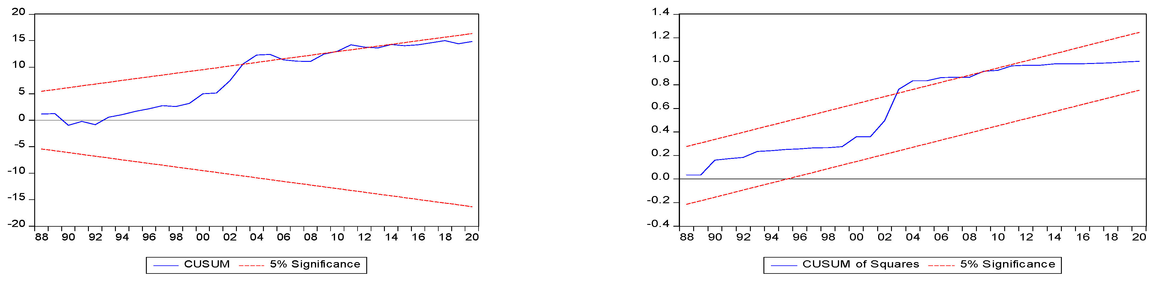
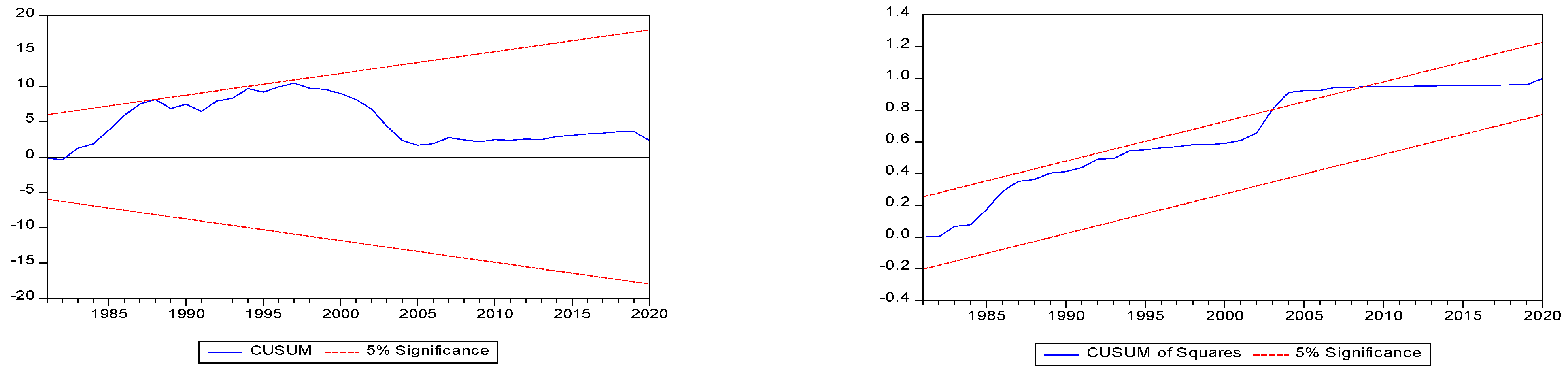
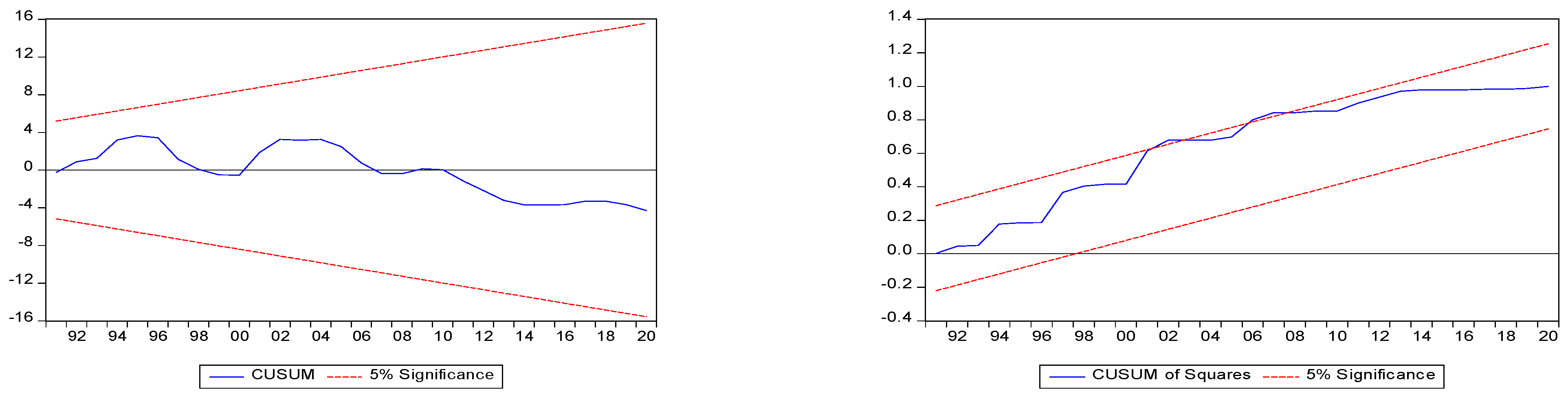
The objective of this study is to investigate the empirical cointegration, long-term and short-term dynamics between carbon emissions, economic growth, urbanization, and foreign trade in China. For this purpose, we selected annual time series data from 1971 to 2019 and used the ARDL method for empirical analysis.

In the long run, carbon emissions, economic growth, and urbanization have insignificant effects on foreign trade. Economic growth and urbanization have a significant mutually reinforcing effect. In addition, urbanization facilitates increased carbon emissions, but excessive carbon emissions suppress urbanization. Similarly, carbon emissions promote economic development, but the increase in carbon emission is restrained through optimization of economic structure and industrial transfer. This shows that there is a “balance” mechanism between urbanization and carbon emission, carbon emission, and economic growth, which can self-regulate. In the short run, carbon emissions and economic growth have a significant path dependency that cannot change abruptly in the short period. There are mutually reinforcing effects between economic growth and carbon emissions, urbanization and carbon emissions, and economic growth and urbanization. Foreign trade hurts carbon emissions in the short term.

This empirical finding can guide China and other economies to formulate effective environmental pollution policies. Firstly, urbanization has led to economic growth, but it has also contributed to environmental pollution. The government should establish a green and low-carbon urbanization model, expand investment in the environmental sector, increase the proportion of renewable energy and clean energy, promote the development of green technologies, and improve the efficiency of energy usage to improve environmental quality. Second, there was an interaction between economic growth and carbon emissions. Policymakers need to improve the coordination between economic growth and carbon emissions, establish a carbon tax and green development subsidy policy, and also introduce green investment into the economy. Finally, the government should optimize the trade structure, restructure foreign investment sectors and regions, and reduce import tariffs on green industries.

This study has some limitations. First, the study is conducted with only China as a case study; in future studies, we will consider adding other developing countries. Second, future research can add more macroeconomic variables (outward direct investment, financial remittances, renewable energy consumption, financial value) for analysis. Finally, future empirical studies may use other econometric models, such as the NARDL model, to further explore the asymmetric relationship between carbon emissions, economic growth, urbanization, and foreign trade.

References

1. Pata, U.K. Renewable energy consumption, urbanization, financial development, income and CO2 emissions in Turkey: Testing EKC hypothesis with structural breaks. J. Clean. Prod. 2018, 187, 770–779. [Google Scholar] [CrossRef]
2. Aslam, B.; Hu, J.; Majeed, M.T.; Andlib, Z.; Ullah, S. Asymmetric macroeconomic determinants of CO2 emission in China and policy approaches. Environ. Sci. Pollut. Res. 2021, 28, 41923–41936. [Google Scholar] [CrossRef] [PubMed]
3. Zhang, N.; Yu, K.; Chen, Z. How does urbanization affect carbon dioxide emissions? A cross-country panel data analysis. Energy Policy 2017, 107, 678–687. [Google Scholar] [CrossRef]
4. Rahman, M.M.; Kashem, M.A. Carbon emissions, energy consumption and industrial growth in Bangladesh: Empirical evidence from ARDL cointegration and Granger causality analysis. Energy Policy 2017, 110, 600–608. [Google Scholar] [CrossRef]
5. Li, X.; Ullah, S. Caring for the environment: How CO2 emissions respond to human capital in BRICS economies? Environ. Sci. Pollut. Res. 2022, 29, 18036–18046. [Google Scholar] [CrossRef]
6. Li, X.; Ozturk, I.; Majeed, M.T.; Hafeez, M.; Ullah, S. Considering the asymmetric effect of financial deepening on environmental quality in BRICS economies: Policy options for the green economy. J. Clean. Prod. 2022, 331, 129909. [Google Scholar] [CrossRef]
7. Grossman, G.M.; Krueger, A.B. Environmental Impacts of a North American Free Trade Agreement; NBER: Cambridge, MA, USA, 1991. [Google Scholar]
8. Panayotou, T. Empirical Tests and Policy Analysis of Environmental Degradation at Different Stages of Economic Development. 1993. Available online: https://ideas.repec.org/p/ilo/ilowps/992927783402676.html (accessed on 2 May 2022).
9. Ozturk, I.; Ullah, S. Does digital financial inclusion matter for economic growth and environmental sustainability in OBRI economies? An empirical analysis. Resour. Conserv. Recycl. 2022, 185, 106489. [Google Scholar] [CrossRef]
10. Yin, Y.; Xiong, X.; Ullah, S.; Sohail, S. Examining the asymmetric socioeconomic determinants of CO2 emissions in China: Challenges and policy implications. Environ. Sci. Pollut. Res. 2021, 28, 57115–57125. [Google Scholar] [CrossRef]
11. Ashena, M.; Shahpari, G. Policy uncertainty, economic activity, and carbon emissions: A nonlinear autoregressive distributed lag approach. Environ. Sci. Pollut. Res. 2022, 29, 52233–52247. [Google Scholar] [CrossRef]
12. Yang, Z.; Cai, J.; Lu, Y.; Zhang, B. The Impact of Economic Growth, Industrial Transition, and Energy Intensity on Carbon Dioxide Emissions in China. Sustainability 2022, 14, 4884. [Google Scholar] [CrossRef]
13. Chen, H.; Tackie, E.A.; Ahakwa, I.; Musah, M.; Salakpi, A.; Alfred, M.; Atingabili, S. Does energy consumption, economic growth, urbanization, and population growth influence carbon emissions in the BRICS? Evidence from panel models robust to cross-sectional dependence and slope heterogeneity. Environ. Sci. Pollut. Res. 2022, 29, 37598–37616. [Google Scholar] [CrossRef] [PubMed]
14. Wang, Y.; Li, L.; Kubota, J.; Han, R.; Zhu, X.; Lu, G. Does urbanization lead to more carbon emission? Evidence from a panel of BRICS countries. Appl. Energy 2016, 168, 375–380. [Google Scholar] [CrossRef]
15. Khan, K.; Su, C.W.; Tao, R.; Hao, L.N. Urbanization and carbon emission: Causality evidence from the new industrialized economies. Environ. Dev. Sustain. 2020, 22, 7193–7213. [Google Scholar] [CrossRef]
16. Stern, D.I. Limits to substitution and irreversibility in production and consumption: A neoclassical interpretation of ecological economics. Ecol. Econ. 1997, 21, 197–215. [Google Scholar] [CrossRef]
17. Stern, D.I. Economic growth and energy. Encycl. Energy 2004, 2, 35–51. [Google Scholar]
18. Anser, M.K.; Alharthi, M.; Aziz, B.; Wasim, S. Impact of urbanization, economic growth, and population size on residential carbon emissions in the SAARC countries. Clean Technol. Environ. Policy 2020, 22, 923–936. [Google Scholar] [CrossRef]
19. Xu, Q.; Dong, Y.X.; Yang, R. Urbanization impact on carbon emissions in the Pearl River Delta region: Kuznets curve relationships. J. Clean. Prod. 2018, 180, 514–523. [Google Scholar] [CrossRef]
20. Prastiyo, S.E.; Hardyastuti, S. How agriculture, manufacture, and urbanization induced carbon emission? The case of Indonesia. Environ. Sci. Pollut. Res. 2020, 27, 42092–42103. [Google Scholar] [CrossRef]
21. Dogan, E.; Turkekul, B. CO2 emissions, real output, energy consumption, trade, urbanization and financial development: Testing the EKC hypothesis for the USA. Environ. Sci. Pollut. Res. 2016, 23, 1203–1213. [Google Scholar] [CrossRef]
22. Ali, H.S.; Abdul-Rahim, A.S.; Ribadu, M.B. Urbanization and carbon dioxide emissions in Singapore: Evidence from the ARDL approach. Environ. Sci. Pollut. Res. 2017, 24, 1967–1974. [Google Scholar] [CrossRef]
23. Ghazouani, T.; Boukhatem, J.; Sam, C.Y. Causal interactions between trade openness, renewable electricity consumption, and economic growth in Asia-Pacific countries: Fresh evidence from a bootstrap ARDL approach. Renew. Sustain. Energy Rev. 2020, 133, 110094. [Google Scholar] [CrossRef]
24. Levchenko, A.A. International trade and institutional change. J. Law Econ. Organ. 2013, 29, 1145–1181. [Google Scholar] [CrossRef]
25. Jafri, M.A.H.; Abbas, S.; Ullah, S. Caring for the environment: Measuring the dynamic impact of remittances and FDI on CO2 emissions in China. Environ. Sci. Pollut. Res. 2022, 29, 9164–9172. [Google Scholar] [CrossRef] [PubMed]
26. Chen, Q.; Löschel, A.; Pei, J.; Peters, G.P.; Xue, J.; Zhao, Z. Processing trade, foreign outsourcing and carbon emissions in China. Struct. Chang. Econ. Dyn. 2019, 49, 1–12. [Google Scholar] [CrossRef]
27. Kirikkaleli, D.; Oyebanji, M.O. Consumption-based carbon emissions, trade, and globalization: An empirical study of Bolivia. Environ. Sci. Pollut. Res. 2022, 29, 29927–29937. [Google Scholar] [CrossRef] [PubMed]
28. Ahmed, Z.; Zhang, B.; Cary, M. Linking economic globalization, economic growth, financial development, and ecological footprint: Evidence from symmetric and asymmetric ARDL. Ecol. Indic. 2021, 121, 107060. [Google Scholar] [CrossRef]
29. Li, Z.; Dong, L.; Zhang, H. China’s 30-year praticipation in international climate governance in retrospect. China Popul. Resour. Environ. 2021, 3109, 202–210. [Google Scholar]
30. Kraft, J.; Kraft, A. On the relationship between energy and GNP. J. Energy Dev. 1978, 3, 401–403. [Google Scholar]
31. Ganda, F. Carbon emissions, diverse energy usage and economic growth in south africa: Investigating existence of the environmental kuznets curve EKC. Environ. Prog. Sustain. Energy 2019, 381, 30–46. [Google Scholar] [CrossRef] [Green Version]
32. Pata, U.K. The effect of urbanization and industrialization on carbon emissions in Turkey: Evidence from ARDL bounds testing procedure. Environ. Sci. Pollut. Res. 2018, 258, 7740–7747. [Google Scholar] [CrossRef] [PubMed]
33. Yao, S.; Zhang, S.; Zhang, X. Renewable energy, carbon emission and economic growth: A revised environmental Kuznets Curve perspective. J. Clean. Prod. 2019, 235, 1338–1352. [Google Scholar] [CrossRef]
34. Kaika, D.; Zervas, E. The Environmental Kuznets Curve EKC theory—Part A: Concept, causes and the CO2 emissions case. Energy Policy 2013, 62, 1392–1402. [Google Scholar] [CrossRef]
35. Lee, S.J.; Yoo, S.H. Energy consumption, CO2 emission, and economic growth: Evidence from Mexico. Energy Sources Part B Econ. Plan. Policy 2016, 118, 711–717. [Google Scholar] [CrossRef]
36. Dimitriadis, D.; Katrakilidis, C.; Karakotsios, A. Investigating the dynamic linkages among carbon dioxide emissions, economic growth, and renewable and non-renewable energy consumption: Evidence from developing countries. Environ. Sci. Pollut. Res. 2021, 2830, 40917–40928. [Google Scholar] [CrossRef] [PubMed]
37. Wang, S.; Li, C. The impact of urbanization on CO2 emissions in China: An empirical study using 1980–2014 provincial data. Environ. Sci. Pollut. Res. 2018, 253, 2457–2465. [Google Scholar] [CrossRef]
38. Zhang, Z.; Huang, H.; Lin, L. Research on the relationship among trade openness, economic growth and carbon emissions: Empirical analysis based on the Belt and Road countries. Soft Sci. 2021, 3510, 44–48. [Google Scholar]
39. Yang, M. Time-varying impact of urbanization on economic growth and carbon emissions. J. Tech. Econ. Manag. 2022, 1, 3–8. [Google Scholar]
40. Qayyum, F.; Mehmood, U.; Tariq, S.; Nawaz, H. Particulate matter PM2.5 and diseases: An autoregressive distributed lag ARDL technique. Environ. Sci. Pollut. Res. 2021, 2847, 67511–67518. [Google Scholar] [CrossRef]
41. Attiaoui, I.; Boufateh, T. Impacts of climate change on cereal farming in Tunisia: A panel ARDL–PMG approach. Environ. Sci. Pollut. Res. 2019, 2613, 13334–13345. [Google Scholar] [CrossRef]
42. Malik, M.Y.; Latif, K.; Khan, Z.; Butt, H.D.; Hussain, M.; Nadeem, M.A. Symmetric and asymmetric impact of oil price, FDI and economic growth on carbon emission in Pakistan: Evidence from ARDL and non-linear ARDL approach. Sci. Total Environ. 2020, 726, 138421. [Google Scholar] [CrossRef]
43. Adom, P.K.; Bekoe, W. Conditional dynamic forecast of electrical energy consumption requirements in Ghana by 2020: A comparison of ARDL and PAM. Energy 2012, 441, 367–380. [Google Scholar] [CrossRef]
44. Shen, Y.; Huang, X.; Liu, L.; Hu, Z.; Gu, J.; Jiang, C.W. Research on forecasting electricity consumption of high-energy-consuming industries based on Granger causality and ARDL model. J. Electr. Power Sci. Technol. 2022, 8, 19–33. [Google Scholar]
45. Bosah, C.P.; Li, S.; Ampofo, G.K.M.; Liu, K. Dynamic nexus between energy consumption, economic growth, and urbanization with carbon emission: Evidence from panel PMG-ARDL estimation. Environ. Sci. Pollut. Res. 2021, 2843, 61201–61212. [Google Scholar] [CrossRef] [PubMed]
46. Wen, H.; Dai, J. Trade openness, environmental regulation, and human capital in China: Based on ARDL cointegration and Granger causality analysis. Environ. Sci. Pollut. Res. 2020, 272, 1789–1799. [Google Scholar] [CrossRef]
47. Charemza, W.W.; Deadman, D.F. New Directions in Econometric Practice; Edward Elgar: London, UK, 1997. [Google Scholar]
48. Pesaran, M.H.; Shin, Y.; Smith, R.P. Pooled mean group estimation of dynamic heterogeneous panels. J. Am. Stat. Assoc. 1999, 94446, 621–634. [Google Scholar] [CrossRef]
49. Peseran, M.H.; Peseran, B. Working with Microfit 4: Interactive Econometric Analysis; Oxford University Press: Oxford, UK, 1997. [Google Scholar]
50. Pesaran, M.H.; Shin, Y.; Smith, R.J. Bounds testing approaches to the analysis of level relationships. J. Appl. Econom. 2001, 163, 289–326. [Google Scholar] [CrossRef]
51. Narayan, P.K. The saving and investment nexus for China: Evidence from cointegration tests. Appl. Econ. 2005, 37, 1979–1990. [Google Scholar] [CrossRef]
52. Liu, W. EKC test study on the relationship between carbon dioxide emission and regional economic growth. Carbon Manag. 2020, 114, 415–425. [Google Scholar] [CrossRef]
53. Sun, Y.; Li, M.; Zhang, M.; Khan, H.S.U.D.; Li, J.; Li, Z.; Sun, H.; Zhu, Y.; Anaba, O.A. A study on China’s economic growth, green energy technology, and carbon emissions based on the Kuznets curve EKC. Environ. Sci. Pollut. Res. 2021, 286, 7200–7211. [Google Scholar] [CrossRef] [PubMed]
54. Yi, Y.; Guan, W.; Gao, Y. Empirical research on the relationship between FDI and CO2 emission in China: The empirical research based on ARDL. J. Guizhou Univ. Financ. Econ. 2015, 3, 58–65. [Google Scholar]
55. Li, K.; Qi, S. Trade openness, economic growth and carbon dioxide emission in China. Econ. Res. J. 2011, 4611, 60–72+102. [Google Scholar]
56. Halicioglu, F. An econometric study of CO2 emissions, energy consumption, income and foreign trade in Turkey. Energy Policy 2009, 373, 1156–1164. [Google Scholar] [CrossRef] [Green Version]
57. Project Synthesis Report Writing Team. Comprehensive Report on China’s Long-term Low-Carbon Development Strategy and Transformation Path Research. China Popul. Resour. Environ. 2020, 30, 1–25. [Google Scholar]
58. Liang, W.; Yang, M. Urbanization, economic growth and environmental pollution: Evidence from China. Sustain. Comput. Inform. Syst. 2019, 21, 1–9. [Google Scholar] [CrossRef]
59. Jiang, A.; Yang, Z. New urbanization construction and high-quality urban economic growth: An empirical analysis based on the double difference method. Inq. Econ. Issues 2020, 3, 84–99. [Google Scholar]
60. Wu, D.; Xu, L.; Yang, Y. The analysis of the impact of China’s foreign trade on economic growth based on the improved two-stage quantile regression for panel data. J. Appl. Stat. Manag. 2019, 4, 571–579. [Google Scholar]
61. Wu, J.; Gao, H. Research on the relationship between economic growth, industrial structure adjustment and urbanization based on VAR model. Macroeconomics 2017, 9, 47–55. [Google Scholar]
Figure 1. The trend of the variable.
Sustainability 14 09396 g001
Figure 2. Test results of explained variable L n C E t .
Sustainability 14 09396 g002
Figure 3. Test results of explained variable L n G D P t .
Sustainability 14 09396 g003
Figure 4. Test results of explained variable L n U B t .
Sustainability 14 09396 g004