Study on Low-Carbon Technology Innovation Strategies through Government–University–Enterprise Cooperation under Carbon Trading Policy

Abstract

This paper focuses on developing low-carbon technology (LCT) innovation in traditional enterprises under carbon trading policies. The Hamilton–Jacobi–Berman equation quantitatively investigates the coordination mechanism and optimal strategy of LCT innovation systems in conventional industries. A three-way dynamic differential game model is constructed to analyze three cases: the Nash disequilibrium game; the Stackelberg master–slave game; and the cooperative game with the optimal effort of universities, traditional enterprises, and local government, the optimal benefits of the three parties, the region, and the regional LCT level. The results are as follows: (1) by changing the government subsidy factor, carbon trading price, and carbon trading tax rate, the optimal effort of universities and traditional enterprises can be significantly increased; (2) cost-sharing contracts do not change the level of effort of local government to manage the environment, and the use of cost-sharing agreements can change the status of action of universities and enterprises; (3) the optimal effort, optimal benefit, and total system benefit of the three parties and the level of LCT of the industry in the cooperative game are better than those in the non-cooperative case. The combined game achieves the Pareto optimum of the system. The study will contribute to both sustainable business development and environmental sustainability.

1. Introduction

The global environment is a total ecosystem, and global warming and resource depletion are becoming a growing concern for people worldwide. Many countries and industries worldwide emphasize low carbon production and are working hard to reduce carbon emissions [1]. 2020 saw the Chinese central government set two primary goals of “carbon peaking” and “carbon neutrality” [2]. In July 2021, China launched the world’s largest carbon trading market to promote the greening and low-carbonization of its industrial structure and energy consumption in high-emission industries to achieve the two goals of “carbon peaking” and “carbon neutrality” [3]. In July 2021, China launched the world’s largest carbon trading market, aiming to promote the green and low-carbon industrial structure and energy consumption of high-emission industries to achieve the two primary goals of “carbon peaking” and “carbon neutrality”. Under the guidance of national policies and the market, production enterprises need to increase their carbon emission reduction efforts and promote green and low-carbon technology (LCT) innovation to achieve near-zero emissions [4]. Enterprises with high LCT will be more competitive in future market competition.

As the main body of regional emission reduction, production enterprises often put their profits first. Not only does it cost a certain amount of money to reduce emissions, but they often sacrifice some of their production capacity; at the same time, production enterprises often have to cooperate with universities to innovate in LCT, and their investment costs are enormous and their returns unpredictable. Therefore, enterprises are not so motivated to take the initiative to reduce emissions. China’s central policies are carbon quotas and carbon trading, which force companies to undertake LCT innovation. The carbon quota policy means enterprises can trade the extra carbon credits for low carbon production under a set carbon quota. If their carbon emissions exceed the set quota, they need to enter the carbon trading market to buy them, and the money spent to buy other companies’ carbon credits is the so-called carbon trading cost [5]. China has already established a national carbon emissions trading system, and many enterprises are actively participating. However, many industries have not yet been included in the carbon emissions trading market, and the carbon emissions trading market is still operating in pilot cities. In addition, if carbon quota policies can be further promoted to limit the carbon emissions of enterprises, this will allow the external environmental costs of the enterprises concerned to be converted into internal costs [6,7], which may further promote LCT innovation and cleaner production methods, which is also essential in promoting carbon emission reduction in China.

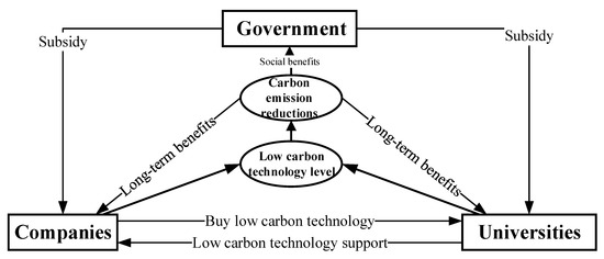
Quantifying the cost of carbon is essential to inform business decision makers. Most existing studies [8,9] only consider the costs associated with business operations, but not the direct economic losses caused by carbon emissions, and most current studies [10,11] only study collaborative innovation systems between governments and enterprises without considering the role of technology suppliers (universities), whereas in practice, the birth of new technology is often the result of collaborative innovation between universities and traditional enterprises led by local government. In China, enterprises often collaborate with universities for technological innovation, and universities are often the suppliers of the most advanced technologies [12]. While other enterprises can also act as carbon capture/elimination/reduction technology providers, the most advanced technology providers are often universities. In addition, collaborative innovation between enterprises and universities has an essential impact on carbon reduction [13], but scholars and government departments have neglected this issue. On the one hand, China’s industry-university research base is weak and has not yet developed a more mature development model; on the other hand, China not only needs to invest more in the short-term effects of technological progress but also needs to achieve a balance between economic growth and environmental protection through technological progress. As technology grows, China will have to deal with the relationship between the economy and the environment, so studying how to promote cooperation between enterprises and universities to improve LCT synergistically will be an essential issue. This paper selects universities, traditional enterprises, and local government as research objects (the specific relationship is shown in Figure 1). A differential game model is used to study low-carbon technological innovation activities under different decision-making scenarios, providing suggestions for governments at all levels, universities, and traditional enterprises from the perspective of sustainable development. At the same time, this study is essential for understanding the relationship between environmental regulation and LCT innovation from a market-oriented perspective.

The remainder of the paper is organized as follows: Section 2 reviews the relevant literature and highlights the innovative aspects of this study. Section 3 makes fundamental assumptions about the model and sets the appropriate parameters. Section 4 constructs three different decision models and analyses the results for the three scenarios. Section 5 uses MATLAB software to simulate the results of the research obtained. Section 6 summarizes the full text and makes the corresponding recommendations.

2. Literature Review

The literature review in this paper consists of three main areas, one on the development of LCT, one on the study of the impact of different national policies on LCT innovation, and the remaining one on the related application of differential game models.

The improvement of LCT can effectively reduce the carbon emissions of production enterprises, which can not only correspond to environmental problems but also promote the sustainable development of enterprises and improve their competitiveness [14]. Although China’s LCT and industries have made significant progress in recent years, there are also many problems. According to a study by the United Nations Development Program [15], China needs to master at least 62 critical specialized and generic technologies in six sectors, namely, electricity, transportation, construction, iron and steel, cement and chemical, and petroleum, to achieve its carbon control and emission reduction targets, and for most of these critical technologies, China does not currently have access to the core technologies [16]. Research institutes and universities mainly dominate the development of LCT in China, and the initiative of enterprises is not strong [17]. Although some large state-owned enterprises have undertaken some of the LCT innovation work under the impetus of national policies, most of the remaining LCT projects are hardly supported by social funding, and the research results cannot be transferred, making the development from theory to application difficult [18,19].

Moreover, LCT in China currently suffers from high costs and low performance improvements. It lacks market competitiveness, making it all the more necessary for the relevant national departments to formulate corresponding policies to promote the innovative development of LCT. Traditional enterprises, universities, and local governments face many issues [20]. Universities provide technology and solutions for enterprises in the process of LCT innovation. Enterprises apply the technologies [21], while the local government offers particular incentives for enterprises to stimulate their enthusiasm, and these three interact with each other. How to determine the subsidy coefficient and the subsidy method is the focus of this paper.

Most scholars have studied national policies’ impact on LCT innovation strategies. Scholars have introduced different perspectives, such as carbon taxes [22], carbon fines [23], and production income taxes [24]. They have demonstrated through specific analyses that these factors impact firms’ LCT innovation choices. Each of these studies has its validity, but there are also limitations. Local governments typically monitor and guide firms’ low-carbon innovation behavior through three types of environmental regulation [25], namely, command-and-control, incentive-based, and voluntary. As mentioned above, a considerable number of studies have introduced different regulatory policies such as carbon taxes, carbon fines, etc., but Kneller and Manderson [26] found that environmental regulation policies did not lead to an increase in R&D investment and had no effect on innovation in LCT; Zhang et al. [27] argued that environmental regulation positively impacts LCT innovation, and firms will actively implement green technology upgrades to reduce pollutant emissions; Cao et al. [28] argued that the relationship between environmental regulation and LCT innovation is uncertain, that green technology progress will only be promoted when the intensity of the regulatory policy reaches a certain threshold, and that the threshold varies for different types of environmental regulatory policies [29]. Suppose the government fails to anticipate changes in the market environment and make the proper policy adjustments. In that case, it will directly affect the implementation of the policy or even lead to policy failure. The existing literature focuses on the impact of command-and-control environmental regulation approaches on LCT innovation and its performance, ignoring the role of incentive-based and voluntary environmental regulation approaches. In addition, the issue of taxation of carbon trading has not been considered in previous papers [30] that introduced carbon trading, neglecting this part of the government’s interest revenue.

In summary, it is not enough to consider a single environmental regulation policy for LCT innovation, but the similar role of multiple environmental regulation policies should be considered. In this paper, I will view not only the command-and-control policy of taxation but also the incentive policy of cost-sharing and the voluntary approach to carbon trading revenue. These three and their enthusiasm and interact with each other. The adoption of different subsidy instruments will be effective in promoting LCT innovation and improving the standard of LCT.

The above analysis shows that there is a game relationship between government and firms in the process of implementing environmental regulation policies. The government has the responsibility to encourage enterprises to innovate [31,32]. The government will choose environmental regulation implementation strategies to attract liquid capital based on enterprises’ preferences. In turn, enterprises will decide whether to engage in LCT innovation based on the magnitude between the costs and benefits of participating in LCT innovation activities [33]. In the process of LCT innovation, universities provide technology to enterprises. The local government will consider giving financial subsidies to enterprises for green production. The three co-exist in the social-ecological system and influence each other. Traditional enterprises, universities, and local government face problems in decision making and distribution of benefits. Static game equilibrium strategies do not adequately reflect the reality of the current situation. Differential games are a standard method for solving time-continuous dynamic game problems and can more realistically reflect the assessment of decisions [34]. The control strategy of carbon emission changes with time, and the differential game model can be used to consider carbon emission reductions. This paper uses differential game theory to study the long-term dynamic interaction mechanism between the government, enterprises, and universities. The government, enterprises, and universities should adjust their decisions according to the changes in the strategies of other participants. The results of the study will help to improve long-term coordination and cooperation between the three parties in the context of carbon reduction, enrich the existing research literature and promote the development of LCT in China to achieve economic growth and environmental sustainability at the same time.

3. Basic Assumptions of the Model

This paper examines the LCT collaborative innovation system among universities, traditional enterprises and local government under limited rationality and proposes the following five hypotheses.

Hypothesis 1.

The level of effort of universities and traditional enterprises in LCT cooperation and innovation is$E_1\left(t\right)$and$E_2\left(t\right)$, respectively. The level of effort of local government in governing the environment is$E_3\left(t\right)$. Considering that the cost of effort of all three parties rises and increases in an increasing trend with their level of activity, with convex characteristics [35], it is assumed that at the moment of$t\in \left[0,+\infty \right]$, the cost function of the participants in the LCT innovation process can be expressed as:

$$C_1\left(E_1\left(t\right)\right)=\frac{1}{2}{\eta }_1{E}_1^2\left(t\right),C_2\left(E_2\left(t\right)\right)=\frac{1}{2}{\eta }_2{E}_2^2\left(t\right),C_3\left(E_3\left(t\right)\right)=\frac{1}{2}{\eta }_3{E}_3^2\left(t\right)$$

(1)

where${\eta }_1>0,{\eta }_2>0,{\eta }_3>0$denote the respective effort cost coefficients of universities, traditional enterprises, and local government, respectively.

Hypothesis 2.

It is assumed that the level of LCT is captured by the variable$x\left(t\right)$, whose derivative$dx\left(t\right)/dt$describes its variation in time$t\in \left[0,+\infty \right]$, as determined by the joint efforts of universities, traditional enterprises, and local government. Furthermore, LCT innovation is a dynamic process of change. As time migrates, the level of LCT in the industry is time-sensitive due to the ageing and obsolescence of existing technologies and the upgrading of new technologies. Therefore, the level of LCT will naturally decline. Combined with previous scholarly research [36], the change in the level of LCT over time can be described by the following stochastic differential equation:

$$\{\begin{array}{c}\dot{x\left(t\right)}=r_1{E}_1\left(t\right)+r_2{E}_2\left(t\right)+r_3{E}_3\left(t\right)-\delta x\left(t\right)\\ x\left(t=0\right)\ge 0\end{array}$$

(2)

where$r_1,r_2,r_3$represent the degree of influence of the efforts of universities, traditional enterprises, and local government to promote cooperative development on the level of LCT, i.e., the coefficient of the effect of the level of LCT;$\delta >0$is a constant coefficient representing the degree of decay in the story of LCT, i.e., the growth of$x\left(t\right)$will gradually slow down as the participants’ efforts increase, i.e., the marginal utility decreases.$x\left(t=0\right)$denotes the initial state of the LCT level.

Hypothesis 3.

Based on the description in the introduction and the literature review, it is known that revenue corresponds to the reduction in carbon emissions by low-carbon production on a specified amount of credits. The income from carbon trading can be portrayed by the following differential Equation [37]:

$$\pi \left(x\left(t\right)\right)=P_{cq}\left[\mu +\tau x\left(t\right)\right]$$

(3)

where$\mu +\tau x\left(t\right)$denotes the increase in carbon emissions through LCT,$P_{cq}$is the carbon trading price,$\tau$denotes the coefficient of the effect of the stock of carbon abatement technologies on carbon emissions, and$\mu$is a positive number.

Hypothesis 4.

Carbon abatement technologies will have a long-term profit impact on the government, universities, and traditional enterprises, such as reducing unit abatement costs, improving the living environment of residents, improving social reputation, etc. [38]. Referring to the idea of the total revenue model for product quality management in the literature [39,40], the complete revenue$R\left(t\right)$of an LCT innovation system with government participation at time t can be expressed as:

$$R\left(t\right)={\epsilon }_1{E}_1\left(t\right)+{\epsilon }_2{E}_2\left(t\right)+{\epsilon }_3{E}_3\left(t\right)+\theta x\left(t\right)$$

(4)

where${\epsilon }_1,{\epsilon }_2$, and${\epsilon }_3$denote the environmental benefits of carbon reduction technologies on society and the long-term benefits of traditional enterprises and universities impact coefficients, respectively, and$\theta$denotes the degree of impact of the level of LCT on total income. As a leader in promoting green and low-carbon development in society, the government will be willing to share part of the costs of LCT innovation of traditional enterprises and universities and encourage traditional enterprises and universities to engage in LCT innovation activities actively. The proportion of the expenses that local governments are willing to share in the process of LCT innovation by traditional enterprises and universities working together is${\beta }_1>0$and${\beta }_2>0$, respectively.

Hypothesis 5.

The total benefits of the system will include income from carbon trading and income from the long-term economic benefits of the three parties, with universities receiving the benefits of LCT transfer, enterprises receiving the revenue from carbon trading and the long-lasting corporate benefits from LCT, and the government receiving the environmental benefits of low-carbon production and the taxes collected from carbon trading. Assuming a specific total revenue, all three would receive a certain proportion of the income, with the balance of profits received by universities and enterprises being${\omega }_1$and${\omega }_2$, and the proportion of profits received by local government being$\left(1-{\omega }_1-{\omega }_2\right)$. All three parties make rational decisions based on complete information. They have the same discount factor$\rho >0$at any moment in an infinite time horizon. Furthermore, all parameters in the model${\epsilon }_1,{\epsilon }_2,{\epsilon }_3,\mu ,{\eta }_1,{\eta }_2,$etc., are time-independent constants. Based on the differential game model, the author has developed different mathematical models for three scenarios, decentralized decision making without cost-sharing, decentralized decision making with cost-sharing, and centralized decision making, and obtained equilibrium results for the government, universities, and traditional enterprises in the following sections.

4. Model Development and Solution

In the previous chapter, the author described the research problem of this paper and made relevant assumptions. In this section, I investigate the impact of carbon trading policies on the optimal strategies of the three parties in decentralized decision making and analyze whether cost-sharing contracts can bring the optimal method of the parties in decentralized decision making to the optimal level in centralized decision making; if not, I further analyze whether and to what extent cost-sharing contracts can bring the optimal decisions of the parties to Pareto Improvement. If this is not the case, further analysis will be undertaken to determine whether and to what extent cost-sharing contracts can lead to a Pareto improvement in the optimal decisions of each party, to provide a basis for decisions to promote LCT cooperation and innovation.

4.1. Costless Decentralised Decision Making (Nash Non-Cooperative Game)

At this point, the local government, the university, and the traditional enterprise are independent and on equal footing. The provincial government does not adopt a subsidy policy, and all parties aim to maximize their interests, i.e., ${\beta }_1={\beta }_2=0$. The functions of local government, universities, and traditional enterprises are expressed as:

$$\begin{array}{c}{\Pi }_1^N={{\displaystyle \int }}_0^{\infty }{e}^{-\rho t}\left\{{\omega }_1\left[{\epsilon }_1{E}_1\left(t\right)+{\epsilon }_2{E}_2\left(t\right)+{\epsilon }_3{E}_3\left(t\right)+\theta x\left(t\right)+P_{cq}\left(\mu +\tau x\right)\right]-\frac{1}{2}{\eta }_1{E}_1^2\left(t\right)\right\}dt\\ {\Pi }_2^N={{\displaystyle \int }}_0^{\infty }{e}^{-\rho t}\left\{{\omega }_2\left[{\epsilon }_1{E}_1\left(t\right)+{\epsilon }_2{E}_2\left(t\right)+{\epsilon }_3{E}_3\left(t\right)+\theta x\left(t\right)+P_{cq}\left(\mu +\tau x\right)\right]-\frac{1}{2}{\eta }_2{E}_2^2\left(t\right)\right\}dt\\ {\Pi }_3^N={{\displaystyle \int }}_0^{\infty }{e}^{-\rho t}\left\{\left(1-{\omega }_1-{\omega }_2\right)\left[{\epsilon }_1{E}_1\left(t\right)+{\epsilon }_2{E}_2\left(t\right)+{\epsilon }_3{E}_3\left(t\right)+\theta x\left(t\right)+P_{cq}\left(\mu +\tau x\right)\right]-\frac{1}{2}{\eta }_3{E}_3^2\left(t\right)\right\}dt\end{array}$$

(5)

To determine the feedback equilibrium strategy for each party, the Hamilton–Jacobi–Bellman equation is solved according to sufficient conditions for the Nash equilibrium with static feedback. The calculation results are shown in Proposition 1.

Proposition 1.

The equilibrium results for the decentralized decision scenario when there is no cost-sharing are as follows:

(1)

The optimal decision for each university, the traditional enterprise, and the local government are:

$$E_1^N=\frac{{\omega }_1\left[{\epsilon }_1\left(\rho +\delta \right)+r_1\left(\theta +\tau P_{cq}\right)\right]}{{\eta }_1\left(\rho +\delta \right)} E_2^N=\frac{{\omega }_2\left[{\epsilon }_2\left(\rho +\delta \right)+r_2\left(\theta +\tau P_{cq}\right)\right]}{{\eta }_2\left(\rho +\delta \right)} E_3^N=\frac{\left(1-{\omega }_1-{\omega }_2\right)[{\epsilon }_3\left(\rho +\delta \right)+r_3\left(\theta +\tau P_{cq}\right)]}{{\eta }_3\left(\rho +\delta \right)}$$

(2)

The optimal trajectory of the optimal LCT stock for this system is $x^N\left(t\right)=\frac{A^N}{\delta }+\left(x_0-\frac{A^N}{\delta }\right)e^{-\delta t}$, where:

$$A^N=\frac{r_1{\omega }_1\left[{\epsilon }_1\left(\rho +\delta \right)+r_1\left(\theta +\tau P_{cq}\right)\right]}{{\eta }_1\left(\rho +\delta \right)}+\frac{r_2{\omega }_2\left[{\epsilon }_2\left(\rho +\delta \right)+r_2\left(\theta +\tau P_{cq}\right)\right]}{{\eta }_2\left(\rho +\delta \right)}+\frac{r_3\left(1-{\omega }_1-{\omega }_2\right)[{\epsilon }_3\left(\rho +\delta \right)+r_3\left(\theta +\tau P_{cq}\right)]}{{\eta }_3\left(\rho +\delta \right)}$$

(3)

The respective profit optimality functions of universities, traditional enterprises, and local government are $V_1^N=k_1^N{x}^N+b_1^N V_2^N=k_2^N{x}^N+b_2^N V_3^N=k_3^N{x}^N+b_3^N$, where$k_1^N=\frac{{\omega }_1\left(\theta +\tau P_{cq}\right)}{\rho +\delta },k_2^N=\frac{{\omega }_2\left(\theta +\tau P_{cq}\right)}{\rho +\delta },k_3^N=\frac{\left(1-{\omega }_1-{\omega }_2\right)\left(\theta +\tau P_{cq}\right)}{\rho +\delta }$,

$$b_1^N=\frac{{\omega }_1\mu P_{cq}}{\rho }+\frac{{\omega }_1{}^2{\left[{\epsilon }_1\left(\rho +\delta \right)+r_1\left(\theta +\tau P_{cq}\right)\right]}^2}{2\rho {\eta }_1{\left(\rho +\delta \right)}^2}+\frac{{\omega }_1{\omega }_2{\left[{\epsilon }_2\left(\rho +\delta \right)+r_2\left(\theta +\tau P_{cq}\right)\right]}^2}{\rho {\eta }_2{\left(\rho +\delta \right)}^2}+\frac{{\omega }_1\left(1-{\omega }_1-{\omega }_2\right){\left[{\epsilon }_3\left(\rho +\delta \right)+r_3\left(\theta +\tau P_{cq}\right)\right]}^2}{\rho {\eta }_3{\left(\rho +\delta \right)}^2}$$

$$b_2^N=\frac{{\omega }_2\mu P_{cq}}{\rho }+\frac{{\omega }_2{}^2{\left[{\epsilon }_2\left(\rho +\delta \right)+r_2\left(\theta +\tau P_{cq}\right)\right]}^2}{2\rho {\eta }_2{\left(\rho +\delta \right)}^2}+\frac{{\omega }_1{\omega }_2{\left[{\epsilon }_1\left(\rho +\delta \right)+r_1\left(\theta +\tau P_{cq}\right)\right]}^2}{\rho {\eta }_1{\left(\rho +\delta \right)}^2}+\frac{{\omega }_2\left(1-{\omega }_1-{\omega }_2\right){\left[{\epsilon }_3\left(\rho +\delta \right)+r_3\left(\theta +\tau P_{cq}\right)\right]}^2}{\rho {\eta }_3{\left(\rho +\delta \right)}^2}$$

$$b_3^N=\frac{\left(1-{\omega }_1-{\omega }_2\right)\mu P_{cq}}{\rho }+\frac{{\left(1-{\omega }_1-{\omega }_2\right)}^2{\left[{\epsilon }_3\left(\rho +\delta \right)+r_3\left(\theta +\tau P_{cq}\right)\right]}^2}{2\rho {\eta }_3{\left(\rho +\delta \right)}^2}+\frac{\left(1-{\omega }_1-{\omega }_2\right){\omega }_1{\left[{\epsilon }_1\left(\rho +\delta \right)+r_1\left(\theta +\tau P_{cq}\right)\right]}^2}{\rho {\eta }_1{\left(\rho +\delta \right)}^2}+\frac{{\omega }_2\left(1-{\omega }_1-{\omega }_2\right){\left[{\epsilon }_2\left(\rho +\delta \right)+r_2\left(\theta +\tau P_{cq}\right)\right]}^2}{\rho {\eta }_2{\left(\rho +\delta \right)}^2}$$

Proof. 

Assume that universities, traditional firms, and local governments have continuous bounded differential revenue functions $V_i^N\left(x\right)\left(iϵ\left\{1,2,3\right\}\right)$ satisfying the HJB equation for $x\ge 0$, i.e.,

$$\rho V_1^N\left(x\right)=\underset{E_1\ge 0}{max}\{{\omega }_1\left[{\epsilon }_1{E}_1+{\epsilon }_2{E}_2+{\epsilon }_3{E}_3+\theta x+P_{cq}\left(\mu +\tau x\right)\right]-\frac{1}{2}{\eta }_1{E}_1^2+\frac{\partial V_1^N}{\partial x}\left(r_1{E}_1+r_2{E}_2+r_3{E}_3-\delta x\right)\}$$

(6)

$$\rho V_2^N\left(x\right)=\underset{E_2\ge 0}{max}\{{\omega }_2\left[{\epsilon }_1{E}_1+{\epsilon }_2{E}_2+{\epsilon }_3{E}_3+\theta x+P_{cq}\left(\mu +\tau x\right)\right]-\frac{1}{2}{\eta }_2{E}_2^2+\frac{\partial V_2^N}{\partial x}\left(r_1{E}_1+r_2{E}_2+r_3{E}_3-\delta x\right)\}$$

(7)

$$\begin{array}{c}\rho V_3^N\left(x\right)=\underset{E_3\ge 0}{max}\{\left(1-{\omega }_1-{\omega }_2\right)\left[{\epsilon }_1{E}_1+{\epsilon }_2{E}_2+{\epsilon }_3{E}_3+\theta x+P_{cq}\left(\mu +\tau x\right)\right]-\frac{1}{2}{\eta }_3{E}_3^2+\frac{\partial V_3^N}{\partial x}\left(r_1{E}_1+r_2{E}_2+r_3{E}_3-\delta x\right)\}\end{array}$$

(8)

The above equations are concave functions with respect to $E_1,E_2$, and $E_3$, respectively. According to the first-order condition, the first-order derivatives of $E_1,E_2$, and $E_3$ are found, and the partial derivatives are set to zero to obtain the strategies for universities, traditional enterprises, and local government as follows:

$$E_1^N=\frac{{\omega }_1{\epsilon }_1+r_1\frac{\partial V_1^N}{\partial x}}{{\eta }_1} E_2^N=\frac{{\omega }_2{\epsilon }_2+r_2\frac{\partial V_2^N}{\partial x}}{{\eta }_2} E_3^N=\frac{\left(1-{\omega }_1-{\omega }_2\right){\epsilon }_3+r_3\frac{\partial V_3^N}{\partial x}}{{\eta }_3}$$

(9)

Substituting the resulting $E_1^N,E_2^N$, and $E_3^N$ into Equations (6)–(8), it can be shown that the optimal linear function of $x$ is the solution of the HJB equation, which is deformed as follows:

$$V_1^N=k_1^N{x}^N+b_1^N{V}_2^N=k_2^N{x}^N+b_2^N{V}_3^N=k_3^N{x}^N+b_3^N$$

(10)

where $k_1^N,k_2^N,k_3^N,b_1^N, b_2^N, b_3^N$ are constants which, after certain simplifications, give the following results:

$$\begin{array}{c}\rho \left(k_1^N{x}^N+b_1^N\right)=\left({\omega }_1\theta +{\omega }_1\tau P_{cq}-\delta k_1^N\right)x^N+{\omega }_1\mu P_{cq}+\frac{{\left({\omega }_1{\epsilon }_1+r_1{k}_1^N\right)}^2}{2{\eta }_1}+\frac{\left({\omega }_1{\epsilon }_2+r_2{k}_1^N\right)\left({\omega }_2{\epsilon }_2+r_2{k}_2^N\right)}{{\eta }_2}\\ \hspace{1em}\hspace{1em}\hspace{1em}\hspace{1em}\hspace{1em}\hspace{1em}\hspace{1em}+\frac{\left({\omega }_1{\epsilon }_3+r_3{k}_1^N\right)\left[\left(1-{\omega }_1-{\omega }_2\right){\epsilon }_3+r_3{k}_3^N\right]}{{\eta }_3}\\ \rho \left(k_2^N{x}^N+b_2^N\right)=\left({\omega }_2\theta +{\omega }_2\tau P_{cq}-\delta k_2^N\right)x^N+{\omega }_2\mu P_{cq}+\frac{{\left({\omega }_2{\epsilon }_2+r_2{k}_2^N\right)}^2}{2{\eta }_2}+\frac{\left({\omega }_2{\epsilon }_1+r_1{k}_2^N\right)\left({\omega }_1{\epsilon }_1+r_1{k}_1^N\right)}{{\eta }_1}\\ \hspace{1em}\hspace{1em}\hspace{1em}\hspace{1em}\hspace{1em}\hspace{1em}\hspace{1em}+\frac{\left({\omega }_2{\epsilon }_3+r_3{k}_2^N\right)\left[\left(1-{\omega }_1-{\omega }_2\right){\epsilon }_3+r_3{k}_3^N\right]}{{\eta }_3}\\ \rho \rho \left(k_3^N{x}^N+b_3^N\right)=\left[\left(1-{\omega }_1-{\omega }_2\right)\left(\theta +\tau P_{cq}\right)-\delta k_3^N\right)]x^N+\left(1-{\omega }_1-{\omega }_2\right)\mu P_{cq}+\frac{{\left[\left(1-{\omega }_1-{\omega }_2\right){\epsilon }_3+r_3{k}_3^N\right]}^2}{2{\eta }_3}\\ \hspace{1em}\hspace{1em}\hspace{1em}\hspace{1em}\hspace{1em}\hspace{1em}\hspace{1em}+\frac{\left[\left(1-{\omega }_1-{\omega }_2\right){\epsilon }_1+r_1{k}_3^N\right]\left({\omega }_1{\epsilon }_1+r_1{k}_1^N\right)}{{\eta }_1}+\frac{\left[\left(1-{\omega }_1-{\omega }_2\right){\epsilon }_2+r_2{k}_3^N\right]\left({\omega }_2{\epsilon }_2+r_2{k}_2^N\right)}{{\eta }_2}\end{array}$$

(11)

By solving Equation (11), we can find that $k_1^N,k_2^N,k_3^N,b_1^N, b_2^N, b_3^N$ have the following values when $x\ge 0$.

$$\{\begin{array}{c}{k}_1^N=\frac{{\omega }_1\left(\theta +\tau P_{cq}\right)}{\rho +\delta },k_2^N=\frac{{\omega }_2\left(\theta +\tau P_{cq}\right)}{\rho +\delta },k_3^N=\frac{\left(1-{\omega }_1-{\omega }_2\right)\left(\theta +\tau P_{cq}\right)}{\rho +\delta },\\ b_1^N=\frac{{\omega }_1\mu P_{cq}}{\rho }+\frac{{\omega }_1{}^2{\left[{\epsilon }_1\left(\rho +\delta \right)+r_1\left(\theta +\tau P_{cq}\right)\right]}^2}{2\rho {\eta }_1{\left(\rho +\delta \right)}^2}+\frac{{\omega }_1{\omega }_2{\left[{\epsilon }_2\left(\rho +\delta \right)+r_2\left(\theta +\tau P_{cq}\right)\right]}^2}{\rho {\eta }_2{\left(\rho +\delta \right)}^2}+\frac{{\omega }_1\left(1-{\omega }_1-{\omega }_2\right){\left[{\epsilon }_3\left(\rho +\delta \right)+r_3\left(\theta +\tau P_{cq}\right)\right]}^2}{\rho {\eta }_3{\left(\rho +\delta \right)}^2}\\ b_2^N=\frac{{\omega }_2\mu P_{cq}}{\rho }+\frac{{\omega }_2{}^2{\left[{\epsilon }_2\left(\rho +\delta \right)+r_2\left(\theta +\tau P_{cq}\right)\right]}^2}{2\rho {\eta }_2{\left(\rho +\delta \right)}^2}+\frac{{\omega }_1{\omega }_2{\left[{\epsilon }_1\left(\rho +\delta \right)+r_1\left(\theta +\tau P_{cq}\right)\right]}^2}{\rho {\eta }_1{\left(\rho +\delta \right)}^2}+\frac{{\omega }_2\left(1-{\omega }_1-{\omega }_2\right){\left[{\epsilon }_3\left(\rho +\delta \right)+r_3\left(\theta +\tau P_{cq}\right)\right]}^2}{\rho {\eta }_3{\left(\rho +\delta \right)}^2}\\ b_3^N=\frac{\left(1-{\omega }_1-{\omega }_2\right)\mu P_{cq}}{\rho }+\frac{{\left(1-{\omega }_1-{\omega }_2\right)}^2{\left[{\epsilon }_3\left(\rho +\delta \right)+r_3\left(\theta +\tau P_{cq}\right)\right]}^2}{2\rho {\eta }_3{\left(\rho +\delta \right)}^2}+\frac{\left(1-{\omega }_1-{\omega }_2\right){\omega }_1{\left[{\epsilon }_1\left(\rho +\delta \right)+r_1\left(\theta +\tau P_{cq}\right)\right]}^2}{\rho {\eta }_1{\left(\rho +\delta \right)}^2}+\frac{{\omega }_2\left(1-{\omega }_1-{\omega }_2\right){\left[{\epsilon }_2\left(\rho +\delta \right)+r_2\left(\theta +\tau P_{cq}\right)\right]}^2}{\rho {\eta }_2{\left(\rho +\delta \right)}^2}\end{array}$$

(12)

Substituting the above equation into Equation (9) gives the values of $E_1^N,E_2^N,E_3^N$, and so, the first part of the proposition is proved. Substituting the above equation into Equation (2), the following equation is obtained:

$$\{\begin{array}{c}\dot{x\left(t\right)}=A^N-\delta x\left(t\right)\\ x\left(t=0\right)=x_0\end{array}$$

(13)

where $A^N=r_1{E}_1^N+r_2{E}_2^N+r_3{E}_3^N=\frac{r_1{\omega }_1\left[{\epsilon }_1\left(\rho +\delta \right)+r_1\left(\theta +\tau P_{cq}\right)\right]}{{\eta }_1\left(\rho +\delta \right)}+\frac{r_2{\omega }_2\left[{\epsilon }_2\left(\rho +\delta \right)+r_2\left(\theta +\tau P_{cq}\right)\right]}{{\eta }_2\left(\rho +\delta \right)}+\frac{r_3\left(1-{\omega }_1-{\omega }_2\right)[{\epsilon }_3\left(\rho +\delta \right)+r_3\left(\theta +\tau P_{cq}\right)]}{{\eta }_3\left(\rho +\delta \right)}$

By solving Equation (13), the optimal LCT stock can be found below:

$$x^N=\frac{A^N}{\delta }+\left(x_0-\frac{A^N}{\delta }\right)e^{-\delta t}$$

(14)

$\{k_1^N,k_2^N,k_3^N,b_1^N, b_2^N, b_3^N\}$ by substituting the values of Equation (10), the respective best interest functions of universities, traditional enterprises, and local government can be found as follows:

$$\begin{array}{c}{V}_1^N\left(x\right)=\frac{{\omega }_1\left(\theta +\tau P_{cq}\right)}{\rho +\delta }{x}^N+\frac{{\omega }_1\mu P_{cq}}{\rho }+\frac{{\omega }_1{}^2{\left[{\epsilon }_1\left(\rho +\delta \right)+r_1\left(\theta +\tau P_{cq}\right)\right]}^2}{2\rho {\eta }_1{\left(\rho +\delta \right)}^2}+\frac{{\omega }_1{\omega }_2{\left[{\epsilon }_2\left(\rho +\delta \right)+r_2\left(\theta +\tau P_{cq}\right)\right]}^2}{\rho {\eta }_2{\left(\rho +\delta \right)}^2}\\ \hspace{1em}\hspace{1em}\hspace{1em}\hspace{1em}\hspace{1em}\hspace{1em}+\frac{{\omega }_1\left(1-{\omega }_1-{\omega }_2\right){\left[{\epsilon }_3\left(\rho +\delta \right)+r_3\left(\theta +\tau P_{cq}\right)\right]}^2}{\rho {\eta }_3{\left(\rho +\delta \right)}^2}\\ V_2^N\left(x\right)=\frac{{\omega }_2\left(\theta +\tau P_{cq}\right)}{\rho +\delta }{x}^N+\frac{{\omega }_2\mu P_{cq}}{\rho }+\frac{{\omega }_2{}^2{\left[{\epsilon }_2\left(\rho +\delta \right)+r_2\left(\theta +\tau P_{cq}\right)\right]}^2}{2\rho {\eta }_2{\left(\rho +\delta \right)}^2}+\frac{{\omega }_1{\omega }_2{\left[{\epsilon }_1\left(\rho +\delta \right)+r_1\left(\theta +\tau P_{cq}\right)\right]}^2}{\rho {\eta }_1{\left(\rho +\delta \right)}^2}\\ \hspace{1em}\hspace{1em}\hspace{1em}\hspace{1em}\hspace{1em}\hspace{1em}+\frac{{\omega }_2\left(1-{\omega }_1-{\omega }_2\right){\left[{\epsilon }_3\left(\rho +\delta \right)+r_3\left(\theta +\tau P_{cq}\right)\right]}^2}{\rho {\eta }_3{\left(\rho +\delta \right)}^2}\\ V_3^N\left(x\right)=\frac{\left(1-{\omega }_1-{\omega }_2\right)\left(\theta +\tau P_{cq}\right)}{\rho +\delta }{x}^N+\frac{\left(1-{\omega }_1-{\omega }_2\right)\mu P_{cq}}{\rho }+\frac{{\left(1-{\omega }_1-{\omega }_2\right)}^2{\left[{\epsilon }_3\left(\rho +\delta \right)+r_3\left(\theta +\tau P_{cq}\right)\right]}^2}{2\rho {\eta }_3{\left(\rho +\delta \right)}^2}\\ \hspace{1em}\hspace{1em}\hspace{1em}\hspace{1em}\hspace{1em}\hspace{1em}+\frac{\left(1-{\omega }_1-{\omega }_2\right){\omega }_1{\left[{\epsilon }_1\left(\rho +\delta \right)+r_1\left(\theta +\tau P_{cq}\right)\right]}^2}{\rho {\eta }_1{\left(\rho +\delta \right)}^2}\\ \hspace{1em}\hspace{1em}\hspace{1em}\hspace{1em}\hspace{1em}\hspace{1em}+\frac{{\omega }_2\left(1-{\omega }_1-{\omega }_2\right){\left[{\epsilon }_2\left(\rho +\delta \right)+r_2\left(\theta +\tau P_{cq}\right)\right]}^2}{\rho {\eta }_2{\left(\rho +\delta \right)}^2}\end{array}$$

(15)

Therefore, in the Nash non-cooperative game model, the optimal aggregate payoff function of the three-party cooperative LCT innovation system can be obtained as follows:

$$\begin{array}{cc}{V}^N\left(x\right)=V_1^N\left(x\right) & +V_2^N\left(x\right)+V_3^N\left(x\right)\\ & =\frac{\left(\theta +\tau P_{cq}\right)}{\rho +\delta }{x}^N+\frac{\mu P_{cq}}{\rho }+\frac{\left(2{\omega }_1-{\omega }_1{}^2\right){\left[{\epsilon }_1\left(\rho +\delta \right)+r_1\left(\theta +\tau P_{cq}\right)\right]}^2}{2\rho {\eta }_1{\left(\rho +\delta \right)}^2}\\ & +\frac{\left(2{\omega }_2-{\omega }_2{}^2\right){\left[{\epsilon }_2\left(\rho +\delta \right)+r_2\left(\theta +\tau P_{cq}\right)\right]}^2}{2\rho {\eta }_2{\left(\rho +\delta \right)}^2}+\frac{\left(1-{\omega }_1-{\omega }_2\right){\left[{\epsilon }_3\left(\rho +\delta \right)+r_3\left(\theta +\tau P_{cq}\right)\right]}^2}{2\rho {\eta }_3{\left(\rho +\delta \right)}^2}\end{array}$$

(16)

□

4.2. Stackelberg Master–Slave Game

In the Stackelberg master–slave game, the local government acts as the leader of LCT innovation, while universities and traditional enterprises are the followers. To encourage universities and traditional enterprises to undertake LCT innovation, the local government provides subsidies to universities and traditional enterprises, respectively. The provincial government first determines the level of effort and the proportion of grants for universities and traditional enterprises; universities and traditional enterprises make corresponding decisions after obtaining information about the local government’s decisions to ensure that their interests are maximized. The provincial government can effectively predict the subsequent choices of universities and traditional enterprises before deciding. The objective function can be expressed as:

$$\begin{array}{c}{\Pi }_1^Y={{\displaystyle \int }}_0^{\infty }{e}^{-\rho t}\{{\omega }_1\left[{\epsilon }_1{E}_1\left(t\right)+{\epsilon }_2{E}_2\left(t\right)+{\epsilon }_3{E}_3\left(t\right)+\theta x\left(t\right)+P_{cq}\left(\mu +\omega x\right)\right]-\frac{1}{2}{\eta }_1{E}_1^2\left(t\right)+\frac{{\beta }_1}{2}{\eta }_1{E}_1^2\left(t\right)\}dt\\ {\Pi }_2^Y={{\displaystyle \int }}_0^{\infty }{e}^{-\rho t}\{{\omega }_2\left[{\epsilon }_1{E}_1\left(t\right)+{\epsilon }_2{E}_2\left(t\right)+{\epsilon }_3{E}_3\left(t\right)+\theta x\left(t\right)+P_{cq}\left(\mu +\omega x\right)\right]-\frac{1}{2}{\eta }_2{E}_2^2\left(t\right)+\frac{{\beta }_2}{2}{\eta }_2{E}_2^2\left(t\right)\}dt\\ {\Pi }_3^Y={{\displaystyle \int }}_0^{\infty }{e}^{-\rho t}\{\left(1-{\omega }_1-{\omega }_2\right)\left[{\epsilon }_1{E}_1\left(t\right)+{\epsilon }_2{E}_2\left(t\right)+{\epsilon }_3{E}_3\left(t\right)+\theta x\left(t\right)+P_{cq}\left(\mu +\omega x\right)\right]-\frac{1}{2}{\eta }_3{E}_3^2\left(t\right)-\frac{{\beta }_1}{2}{\eta }_1{E}_1^2\left(t\right)-\frac{{\beta }_2}{2}{\eta }_2{E}_2^2\left(t\right)\}dt\end{array}$$

(17)

Proposition 2.

The equilibrium results for the decentralized decision scenario when there is cost-sharing are as follows:

(1)

The optimal decision and cost-sharing ratio for each university, traditional enterprise, and local government are:

$$\begin{array}{c}{E}_1^Y=\frac{{\omega }_1\left[{\epsilon }_1\left(\rho +\delta \right)+r_1\left(\theta +\tau P_{cq}\right)\right]}{{\eta }_1\left(1-{\beta }_1\right)\left(\rho +\delta \right)}, E_2^Y=\frac{{\omega }_2\left[{\epsilon }_2\left(\rho +\delta \right)+r_2\left(\theta +\tau P_{cq}\right)\right]}{{\eta }_2\left(1-{\beta }_2\right)\left(\rho +\delta \right)},E_3^Y=\frac{\left(1-{\omega }_1-{\omega }_2\right)[{\epsilon }_3\left(\rho +\delta \right)+r_3\left(\theta +\tau P_{cq}\right)]}{{\eta }_3\left(\rho +\delta \right)}\\ {\beta }_1=\frac{2-3{\omega }_1-2{\omega }_2}{2-{\omega }_1-2{\omega }_2}{\beta }_2=\frac{2-3{\omega }_2-2{\omega }_1}{2-{\omega }_2-2{\omega }_1}\end{array}$$

(2)

The optimal trajectory of the optimal LCT stock for this system is $x^Y\left(t\right)=\frac{A^Y}{\delta }+\left(x_0-\frac{A^Y}{\delta }\right)e^{-\delta t}$, where

$$A^Y=r_1\frac{{\omega }_1{\epsilon }_1\left(\rho +\delta \right)+r_1{\omega }_1\left(\theta +\tau P_{cq}\right)}{{\eta }_1\left(1-{\beta }_1\right)\left(\rho +\delta \right)}+r_2\frac{{\omega }_2{\epsilon }_2\left(\rho +\delta \right)+r_2{\omega }_2\left(\theta +\tau P_{cq}\right)}{{\eta }_2\left(1-{\beta }_2\right)\left(\rho +\delta \right)}+r_3\frac{\left(1-{\omega }_1-{\omega }_2\right)[{\epsilon }_3\left(\rho +\delta \right)+r_3\left(\theta +\tau P_{cq}\right)]}{{\eta }_3\left(\rho +\delta \right)}$$

(3)

The respective profit optimal value functions of universities, traditional enterprises, and local government are $V_1^Y=k_1^Y{x}^Y+b_1^Y{V}_2^Y=k_2^Y{x}^Y+b_2^Y V_3^Y=k_3^Y{x}^Y+b_3^Y$, where$k_1^Y=\frac{{\omega }_1\left(\theta +\tau P_{cq}\right)}{\rho +\delta },k_2^Y=\frac{{\omega }_2\left(\theta +\tau P_{cq}\right)}{\rho +\delta },k_3^Y=\frac{\left(1-{\omega }_1-{\omega }_2\right)\left(\theta +\tau P_{cq}\right)}{\rho +\delta }$:

$$b_1^Y=\frac{{\omega }_1\mu P_{cq}}{\rho }+\frac{{\omega }_1\left(2-{\omega }_1-2{\omega }_2\right){\left[{\epsilon }_1\left(\rho +\delta \right)+r_1\left(\theta +\tau P_{cq}\right)\right]}^2}{4\rho {\eta }_1{\left(\rho +\delta \right)}^2}+\frac{{\omega }_1\left(2-{\omega }_2-2{\omega }_1\right){\left[{\epsilon }_2\left(\rho +\delta \right)+r_2\left(\theta +\tau P_{cq}\right)\right]}^2}{2\rho {\eta }_2{\left(\rho +\delta \right)}^2}+\frac{{\omega }_1\left(1-{\omega }_1-{\omega }_2\right){\left[{\epsilon }_3\left(\rho +\delta \right)+r_3\left(\theta +\tau P_{cq}\right)\right]}^2}{\rho {\eta }_3{\left(\rho +\delta \right)}^2}$$

$$b_2^Y=\frac{{\omega }_2\mu P_{cq}}{\rho }+\frac{{\omega }_2\left(2-2{\omega }_1-{\omega }_2\right){\left[{\epsilon }_2\left(\rho +\delta \right)+r_2\left(\theta +\tau P_{cq}\right)\right]}^2}{4\rho {\eta }_2{\left(\rho +\delta \right)}^2}+\frac{{\omega }_2\left(2-{\omega }_1-2{\omega }_2\right){\left[{\epsilon }_1\left(\rho +\delta \right)+r_1\left(\theta +\tau P_{cq}\right)\right]}^2}{2\rho {\eta }_1{\left(\rho +\delta \right)}^2}+\frac{{\omega }_2\left(1-{\omega }_1-{\omega }_2\right){\left[{\epsilon }_3\left(\rho +\delta \right)+r_3\left(\theta +\tau P_{cq}\right)\right]}^2}{\rho {\eta }_3{\left(\rho +\delta \right)}^2}$$

$$b_3^Y=\frac{\left(1-{\omega }_1-{\omega }_2\right)\mu P_{cq}}{\rho }+\frac{{\left(1-{\omega }_1-{\omega }_2\right)}^2{\left[{\epsilon }_3\left(\rho +\delta \right)+r_3\left(\theta +\tau P_{cq}\right)\right]}^2}{2\rho {\eta }_3{\left(\rho +\delta \right)}^2}+\frac{{\left(2-{\omega }_1-2{\omega }_2\right)}^2{\left[{\epsilon }_1\left(\rho +\delta \right)+r_1\left(\theta +\tau P_{cq}\right)\right]}^2}{8\rho {\eta }_1{\left(\rho +\delta \right)}^2}+\frac{{\left(2-{\omega }_2-2{\omega }_1\right)}^2{\left[{\epsilon }_2\left(\rho +\delta \right)+r_2\left(\theta +\tau P_{cq}\right)\right]}^2}{8\rho {\eta }_2{\left(\rho +\delta \right)}^2}$$

Proof. 

Assume that universities, traditional enterprises and local government have continuous bounded differential revenue functions $V_i^Y\left(x\right)\left(iϵ\left\{1,2,3\right\}\right)$ satisfying the HJB equation for $x\ge 0$. The optimal decision problem for universities and traditional firms is first solved by reverse induction, which yields:

$$\rho V_1^Y\left(x\right)=\underset{E_1\ge 0}{max}\{{\omega }_1\left[{\epsilon }_1{E}_1+{\epsilon }_2{E}_2+{\epsilon }_3{E}_3+\theta x+P_{cq}\left(\mu +\tau x\right)\right]-\frac{\left(1-{\beta }_1\right)}{2}{\eta }_1{E}_1^2+\frac{\partial V_1^Y}{\partial x}\left(r_1{E}_1+r_2{E}_2+r_3{E}_3-\delta x\right)\}$$

(18)

$$\rho V_2^Y\left(x\right)=\underset{E_2\ge 0}{max}\{{\omega }_2\left[{\epsilon }_1{E}_1+{\epsilon }_2{E}_2+{\epsilon }_3{E}_3+\theta x+P_{cq}\left(\mu +\tau x\right)\right]-\frac{\left(1-{\beta }_2\right)}{2}{\eta }_2{E}_2^2+\frac{\partial V_2^Y}{\partial x}\left(r_1{E}_1+r_2{E}_2+r_3{E}_3-\delta x\right)\}$$

(19)

The above equations are concave functions with respect to $E_1,E_2$, respectively. According to the first-order condition, the first-order derivatives of $E_1,E_2$ and letting the partial derivative be 0, we can obtain the optimal strategies of universities and traditional enterprises as follows:

$$E_1^Y=\frac{{\omega }_1{\epsilon }_1+r_1\frac{\partial V_1^Y}{\partial x}}{{\eta }_1\left(1-{\beta }_1\right)} E_2^Y=\frac{{\omega }_2{\epsilon }_2+r_2\frac{\partial V_2^Y}{\partial x}}{{\eta }_2\left(1-{\beta }_2\right)}$$

(20)

As rational decision makers, local governments can predict the optimal strategic choices of universities and enterprises. The local government will determine their optimal strategies, subsidy ratios based on the response functions of universities and traditional enterprises (21). The HJB equation for local governance can be expressed as:

$$\begin{array}{c}\rho V_3^Y\left(x\right)=\underset{E_3\ge 0}{max}\{\left(1-{\omega }_1-{\omega }_2\right)\left[{\epsilon }_1{E}_1+{\epsilon }_2{E}_2+{\epsilon }_3{E}_3+\theta x+P_{cq}\left(\mu +\tau x\right)\right]-\frac{1}{2}{\eta }_3{E}_3^2-\frac{{\beta }_1}{2}{\eta }_1{E}_1^2-\frac{{\beta }_2}{2}{\eta }_2{E}_2^2+\frac{\partial V_3^Y}{\partial x}\left(r_1{E}_1+r_2{E}_2+r_3{E}_3-\delta x\right)\}\end{array}$$

(21)

Substituting Equation (20) into Equation (21) and finding the first-order partial derivatives for $E_3,{\beta }_1,{\beta }_2$ according to the first-order condition and making the partial derivative zero, the optimal strategy for the local government is obtained as follows:

$$\begin{array}{c}{E}_3^Y=\frac{\left(1-{\omega }_1-{\omega }_2\right){\epsilon }_3+r_3\frac{\partial V_3^Y}{\partial x}}{{\eta }_3},{\beta }_1=\frac{{\epsilon }_1\left(2-3{\omega }_1-2{\omega }_2\right)+2r_1\frac{\partial V_3^Y}{\partial x}-r_1\frac{\partial V_1^Y}{\partial x}}{{\epsilon }_1\left(2-{\omega }_1-2{\omega }_2\right)+2r_1\frac{\partial V_3^Y}{\partial x}+r_1\frac{\partial V_1^Y}{\partial x}},\\ {\beta }_2=\frac{{\epsilon }_2\left(2-3{\omega }_2-2{\omega }_1\right)+2r_2\frac{\partial V_3^Y}{\partial x}-r_2\frac{\partial V_2^Y}{\partial x}}{{\epsilon }_2\left(2-{\omega }_2-2{\omega }_1\right)+2r_2\frac{\partial V_3^Y}{\partial x}+r_2\frac{\partial V_2^Y}{\partial x}}\end{array}$$

(22)

Substituting $E_1,E_2,E_3,{\beta }_1,$ and ${\beta }_2$ into Equations (19), (20), and (22). It can be shown that the optimal linear function of $x$ is the solution of the HJB equation, which is deformed as follows:

$$V_1^Y=k_1^Y{x}^Y+b_1^Y V_2^Y=k_2^Y{x}^Y+b_2^Y V_3^Y=k_3^Y{x}^Y+b_3^Y$$

(23)

where $k_1^Y,k_2^Y,k_3^Y,b_1^Y, b_2^Y, b_3^Y$ are constants, which, after simplification, gives the following equation:

$$\begin{array}{c}\rho \left(k_1^Y{x}^Y+b_1^Y\right)=\left[{\omega }_1\left(\theta +\tau P_{cq}\right)-\delta k_1^Y\right]x^Y+\mu {\omega }_1{P}_{cq}+\frac{({\omega }_1{\epsilon }_1+r_1{k}_1^Y)\left[\left(2-{\omega }_1-2{\omega }_2\right){\epsilon }_1+2r_1{k}_3^Y+r_1{k}_1^Y\right]}{4{\eta }_1}\\ \hspace{1em}\hspace{1em}\hspace{1em}\hspace{1em}\hspace{1em}\hspace{1em}+\frac{\left({\omega }_1{\epsilon }_2+r_2{k}_1^Y\right)\left[\left(2-{\omega }_2-2{\omega }_1\right){\epsilon }_2+2r_2{k}_3^Y+r_2{k}_2^Y\right]}{2{\eta }_2}\\ \hspace{1em}\hspace{1em}\hspace{1em}\hspace{1em}\hspace{1em}\hspace{1em}+\frac{\left({\omega }_1{\epsilon }_3+r_3{k}_1^Y\right)\left[\left(1-{\omega }_1-{\omega }_2\right){\epsilon }_3+r_3{k}_3^Y\right]}{{\eta }_3}\\ \rho \left(k_2^Y{x}^Y+b_2^Y\right)=\left[{\omega }_2\left(\theta +\tau P_{cq}\right)-\delta k_2^Y\right]x^Y+\mu {\omega }_2{P}_{cq}+\frac{({\omega }_2{\epsilon }_2+r_2{k}_2^Y)\left[\left(2-{\omega }_2-2{\omega }_1\right){\epsilon }_2+2r_2{k}_3^Y+r_2{k}_2^Y\right]}{4{\eta }_2}\\ \hspace{1em}\hspace{1em}\hspace{1em}\hspace{1em}\hspace{1em}\hspace{1em}+\frac{\left({\omega }_2{\epsilon }_1+r_1{k}_2^Y\right)\left[\left(2-{\omega }_1-2{\omega }_2\right){\epsilon }_1+2r_1{k}_3^Y+r_1{k}_1^Y\right]}{2{\eta }_1}\\ \hspace{1em}\hspace{1em}\hspace{1em}\hspace{1em}\hspace{1em}\hspace{1em}+\frac{\left({\omega }_2{\epsilon }_3+r_3{k}_2^Y\right)\left[\left(1-{\omega }_1-{\omega }_2\right){\epsilon }_3+r_3{k}_3^Y\right]}{{\eta }_3}\\ \rho \left(k_3^Y{x}^Y+b_3^Y\right)=\left[\left(1-{\omega }_1-{\omega }_2\right)\left(\theta +\tau P_{cq}\right)-\delta k_3^Y\right]x^Y+\mu \left(1-{\omega }_1-{\omega }_2\right)P_{cq}+\frac{{\left[\left(1-{\omega }_1-{\omega }_2\right){\epsilon }_3+r_3{k}_3^Y\right]}^2}{2{\eta }_3}\\ \hspace{1em}\hspace{1em}\hspace{1em}\hspace{1em}\hspace{1em}\hspace{1em}+\frac{{\left[\left(2-{\omega }_1-2{\omega }_2\right){\epsilon }_1+2r_1{k}_3^Y+r_1{k}_1^Y\right]}^2}{8{\eta }_1}+\frac{{\left[\left(2-{\omega }_2-2{\omega }_1\right){\epsilon }_2+2r_2{k}_3^Y+r_2{k}_2^Y\right]}^2}{8{\eta }_2}\end{array}$$

(24)

By solving Equation (24), we can find that when $\mathrm{x}\ge 0$, $k_1^Y,k_2^Y,k_3^Y,b_1^Y, b_2^Y, b_3^Y$ have the following values:

$$\{\begin{array}{c}{k}_1^Y=\frac{{\omega }_1\left(\theta +\tau P_{cq}\right)}{\rho +\delta },k_2^Y=\frac{{\omega }_2\left(\theta +\tau P_{cq}\right)}{\rho +\delta },k_3^Y=\frac{\left(1-{\omega }_1-{\omega }_2\right)\left(\theta +\tau P_{cq}\right)}{\rho +\delta }, \\ b_1^Y=\frac{{\omega }_1\mu P_{cq}}{\rho }+\frac{{\omega }_1\left(2-{\omega }_1-2{\omega }_2\right){\left[{\epsilon }_1\left(\rho +\delta \right)+r_1\left(\theta +\tau P_{cq}\right)\right]}^2}{4\rho {\eta }_1{\left(\rho +\delta \right)}^2}+\frac{{\omega }_1\left(2-{\omega }_2-2{\omega }_1\right){\left[{\epsilon }_2\left(\rho +\delta \right)+r_2\left(\theta +\tau P_{cq}\right)\right]}^2}{2\rho {\eta }_2{\left(\rho +\delta \right)}^2}+\frac{{\omega }_1\left(1-{\omega }_1-{\omega }_2\right){\left[{\epsilon }_3\left(\rho +\delta \right)+r_3\left(\theta +\tau P_{cq}\right)\right]}^2}{\rho {\eta }_3{\left(\rho +\delta \right)}^2}\\ b_2^Y=\frac{{\omega }_2\mu P_{cq}}{\rho }+\frac{{\omega }_2\left(2-2{\omega }_1-{\omega }_2\right){\left[{\epsilon }_2\left(\rho +\delta \right)+r_2\left(\theta +\tau P_{cq}\right)\right]}^2}{4\rho {\eta }_2{\left(\rho +\delta \right)}^2}+\frac{{\omega }_2\left(2-{\omega }_1-2{\omega }_2\right){\left[{\epsilon }_1\left(\rho +\delta \right)+r_1\left(\theta +\tau P_{cq}\right)\right]}^2}{2\rho {\eta }_1{\left(\rho +\delta \right)}^2}+\frac{{\omega }_2\left(1-{\omega }_1-{\omega }_2\right){\left[{\epsilon }_3\left(\rho +\delta \right)+r_3\left(\theta +\tau P_{cq}\right)\right]}^2}{\rho {\eta }_3{\left(\rho +\delta \right)}^2}\\ b_3^Y=\frac{\left(1-{\omega }_1-{\omega }_2\right)\mu P_{cq}}{\rho }+\frac{{\left(1-{\omega }_1-{\omega }_2\right)}^2{\left[{\epsilon }_3\left(\rho +\delta \right)+r_3\left(\theta +\tau P_{cq}\right)\right]}^2}{2\rho {\eta }_3{\left(\rho +\delta \right)}^2}+\frac{{\left(2-{\omega }_1-2{\omega }_2\right)}^2{\left[{\epsilon }_1\left(\rho +\delta \right)+r_1\left(\theta +\tau P_{cq}\right)\right]}^2}{8\rho {\eta }_1{\left(\rho +\delta \right)}^2}+\frac{{\left(2-{\omega }_2-2{\omega }_1\right)}^2{\left[{\epsilon }_2\left(\rho +\delta \right)+r_2\left(\theta +\tau P_{cq}\right)\right]}^2}{8\rho {\eta }_2{\left(\rho +\delta \right)}^2}\end{array}$$

(25)

The values of $k_1^Y,k_2^Y$, and $k_3^Y$ were substituted into Equations (20) and (22). The optimal strategies $k_1^Y,k_2^Y$, and $k_3^Y$ for universities, traditional enterprises, and local government are obtained, as well as the optimal subsidies from local government to universities and traditional firms with optimal subsidy coefficients ${\beta }_1$ and ${\beta }_2$. Proposition 2 can be proven. We can obtain:

$$\{\begin{array}{c}\dot{x\left(t\right)}=A^Y-\delta x\left(t\right)\\ x\left(t=0\right)=x_0\end{array}$$

(26)

where $A^Y=r_1{E}_1^Y+r_2{E}_2^Y+r_3{E}_3^Y=\frac{r_1{\omega }_1\left[{\epsilon }_1\left(\rho +\delta \right)+r_1\left(\theta +\tau P_{cq}\right)\right]}{{\eta }_1\left(\rho +\delta \right)}+\frac{r_2{\omega }_2\left[{\epsilon }_2\left(\rho +\delta \right)+r_2\left(\theta +\tau P_{cq}\right)\right]}{{\eta }_2\left(\rho +\delta \right)}+\frac{r_3\left(1-{\omega }_1-{\omega }_2\right)[{\epsilon }_3\left(\rho +\delta \right)+r_3\left(\theta +\tau P_{cq}\right)]}{{\eta }_3\left(\rho +\delta \right)}$.

By solving Equation (26), the optimal LCT stock can be found below:

$$x^Y=\frac{A^Y}{\delta }+\left(x_0-\frac{A^Y}{\delta }\right)e^{-\delta t}$$

(27)

$k_1^Y,k_2^Y,k_3^Y,b_1^Y, b_2^Y, b_3^Y$ by substituting the values of Equation (23), the respective best interest functions of universities, traditional enterprises, and local government can be found as follows:

$$\begin{array}{c}{V}_1^Y\left(x\right)=\frac{{\omega }_1\left(\theta +\tau P_{cq}\right)}{\rho +\delta }{x}^Y+\frac{{\omega }_1\mu P_{cq}}{\rho }+\frac{{\omega }_1\left(2-{\omega }_1-2{\omega }_2\right){\left[{\epsilon }_1\left(\rho +\delta \right)+r_1\left(\theta +\tau P_{cq}\right)\right]}^2}{4\rho {\eta }_1{\left(\rho +\delta \right)}^2}+\frac{{\omega }_1\left(2-{\omega }_2-2{\omega }_1\right){\left[{\epsilon }_2\left(\rho +\delta \right)+r_2\left(\theta +\tau P_{cq}\right)\right]}^2}{2\rho {\eta }_2{\left(\rho +\delta \right)}^2}\\ \hspace{1em}\hspace{1em}\hspace{1em}\hspace{1em}\hspace{1em}\hspace{1em}+\frac{{\omega }_1\left(1-{\omega }_1-{\omega }_2\right){\left[{\epsilon }_3\left(\rho +\delta \right)+r_3\left(\theta +\tau P_{cq}\right)\right]}^2}{\rho {\eta }_3{\left(\rho +\delta \right)}^2}\\ V_2^Y\left(x\right)=\frac{{\omega }_2{(\theta +\tau P}_{cq})}{\rho +\delta }{x}^Y+\frac{{\omega }_2{\mu P}_{cq}}{\rho }+\frac{{\omega }_2{(2-2\omega }_1{-\omega }_2{\left)\right[\epsilon }_2{(\rho +\delta )+r}_2{(\theta +\tau P}_{cq}{\left)\right]}^2}{{4\rho \eta }_2{\left(\rho +\delta \right)}^2}+\frac{{\omega }_2\left({2-\omega }_1{-2\omega }_2\right){{[\epsilon }_1{(\rho +\delta )+r}_1{(\theta +\tau P}_{cq}\left)\right]}^2}{{2\rho \eta }_1{\left(\rho +\delta \right)}^2}+\frac{{\omega }_2{(1-\omega }_1{-\omega }_2{\left)\right[\epsilon }_3{(\rho +\delta )+r}_3{(\theta +\tau P}_{cq}{\left)\right]}^2}{{\rho \eta }_3{\left(\rho +\delta \right)}^2}\\ V_3^Y\left(x\right)=\frac{{(1-\omega }_1{-\omega }_2{\left)\right(\theta +\tau P}_{cq})}{\rho +\delta }{x}^Y+\frac{{(1-\omega }_1{-\omega }_2{)\mu P}_{cq}}{\rho }+\frac{{{(1-\omega }_1{-\omega }_2)}^2{{[\epsilon }_3{(\rho +\delta )+r}_3{(\theta +\tau P}_{cq}\left)\right]}^2}{{2\rho \eta }_3{\left(\rho +\delta \right)}^2}+\frac{{\left({2-\omega }_1{-2\omega }_2\right)}^2{{[\epsilon }_1{(\rho +\delta )+r}_1{(\theta +\tau P}_{cq}\left)\right]}^2}{{8\rho \eta }_1{\left(\rho +\delta \right)}^2}+\frac{{\left({2-\omega }_2{-2\omega }_1\right)}^2{{[\epsilon }_2{(\rho +\delta )+r}_2{(\theta +\tau P}_{cq}\left)\right]}^2}{{8\rho \eta }_2{\left(\rho +\delta \right)}^2}\end{array}$$

(28)

Therefore, in the Stackelberg master–slave game model, the optimal aggregate payoff function for the three-party cooperative LCT innovation system can be obtained as follows:

$$\begin{array}{c}{V}^Y\left(x\right)=V_1^Y\left(x\right)+V_2^Y\left(x\right)+V_3^Y\left(x\right)=\frac{\left(\theta +\tau P_{cq}\right)}{\rho +\delta }{x}^Y+\frac{\mu P_{cq}}{\rho }+\frac{\left(2+{\omega }_1+2{\omega }_2\right)\left(2-{\omega }_1-2{\omega }_2\right){\left[{\epsilon }_1\left(\rho +\delta \right)+r_1\left(\theta +\tau P_{cq}\right)\right]}^2}{8\rho {\eta }_1{\left(\rho +\delta \right)}^2}\\ +\frac{{(2+2\omega }_1{+\omega }_2{\left)\right(2-2\omega }_1{-\omega }_2{\left)\right[\epsilon }_2{(\rho +\delta )+r}_2{(\theta +\tau P}_{cq}{\left)\right]}^2}{{8\rho \eta }_2{\left(\rho +\delta \right)}^2}+\frac{{(1+\omega }_1{+\omega }_2{\left)\right(1-\omega }_1{-\omega }_2{\left)\right[\epsilon }_3{(\rho +\delta )+r}_3{(\theta +\tau P}_{cq}{\left)\right]}^2}{{2\rho \eta }_3{\left(\rho +\delta \right)}^2}\end{array}$$

(29)

□

4.3. Centralised Decision Making (Collaborative, Cooperative Game)

To further promote the low carbon transformation of industries, improve the development of LCT in the region, the relationship between universities, traditional enterprises, and local government is strengthened. The study then moves from a model of government subsidies supporting industry to a tripartite cooperation model. In this case, universities, traditional enterprises, and local government work together as an organic whole to maximize the benefits of the collaborative LCT system and jointly determine the best-effort strategy for the three parties:

$$\begin{array}{c}\Pi ={\Pi }_1+{\Pi }_2+{\Pi }_3\\ ={{\displaystyle \int }}_0^{\infty }{e}^{-\rho t}\left\{\left[{\epsilon }_1{E}_1\left(t\right)+{\epsilon }_2{E}_2\left(t\right)+{\epsilon }_3{E}_3\left(t\right)+\theta x\left(t\right)+P_{cq}\left(\mu +\omega x\right)\right]-\frac{1}{2}{\eta }_3{E}_3^2\left(t\right)-\frac{1}{2}{\eta }_1{E}_1^2\left(t\right)-\frac{1}{2}{\eta }_2{E}_2^2\left(t\right)\right\}dt\end{array}$$

(30)

Proposition 3.

In the case of a cooperative game, the equilibrium results are as follows:

(1)

The optimal decision of each university, the traditional enterprise. and the local government is:

$$E_1^C=\frac{{\epsilon }_1\left(\rho +\delta \right)+r_1\left(\theta +\tau P_{cq}\right)}{{\eta }_1\left(\rho +\delta \right)} E_2^C=\frac{{\epsilon }_2\left(\rho +\delta \right)+r_2\left(\theta +\tau P_{cq}\right)}{{\eta }_2\left(\rho +\delta \right)} E_3^C=\frac{{\epsilon }_3\left(\rho +\delta \right)+r_3\left(\theta +\tau P_{cq}\right)}{{\eta }_3\left(\rho +\delta \right)}$$

(2)

The optimal trajectory of the optimal stock of LCT for this system is $x^C\left(t\right)=\frac{A^C}{\delta }+\left(x_0-\frac{A^C}{\delta }\right)e^{-\delta t}$where$A^C=\frac{r_1[{\epsilon }_1\left(\rho +\delta \right)+r_1\left(\theta +\tau P_{cq}\right)]}{{\eta }_1\left(\rho +\delta \right)}+\frac{r_2\left[{\epsilon }_2\left(\rho +\delta \right)+r_2\left(\theta +\tau P_{cq}\right)\right]}{{\eta }_2\left(\rho +\delta \right)}+\frac{r_3\left[{\epsilon }_3\left(\rho +\delta \right)+r_3\left(\theta +\tau P_{cq}\right)\right]}{{\eta }_3\left(\rho +\delta \right)}$.

(3)

The respective profit optimality functions of universities, traditional firms, and local government are $V^C=k^C{x}^C+b^C$, where $k^C=\frac{\theta +\tau P_{cq}}{\rho +\delta }$,$b^C=\frac{\mu P_{cq}}{\rho }+\frac{{\left[{\epsilon }_1\left(\rho +\delta \right)+r_1\left(\theta +\tau P_{cq}\right)\right]}^2}{2\rho {\eta }_1{\left(\rho +\delta \right)}^2}+\frac{{\left[{\epsilon }_2\left(\rho +\delta \right)+r_2\left(\theta +\tau P_{cq}\right)\right]}^2}{2\rho {\eta }_2{\left(\rho +\delta \right)}^2}+\frac{{\left[{\epsilon }_3\left(\rho +\delta \right)+r_3\left(\theta +\tau P_{cq}\right)\right]}^2}{2\rho {\eta }_3{\left(\rho +\delta \right)}^2}$.

Proof. 

Suppose that the cooperative low-carbon innovation system has a continuous bounded differential payoff function $V^C\left(x\right)$ satisfying the HJB equation for $x\ge 0$, i.e.,

$$\rho V^C\left(x\right)=\underset{E_1\ge 0,E_2\ge 0,E_3\ge 0}{max}\{[{\epsilon }_1{E}_1+{\epsilon }_2{E}_2+{\epsilon }_3{E}_3+\theta x+P_{cq}\left(\mu +\tau x\right)]-\frac{1}{2}{\eta }_3{E}_3^2-\frac{1}{2}{\eta }_1{E}_1^2-\frac{1}{2}{\eta }_2{E}_2^2+\frac{\partial V^C}{\partial x}\left(r_1{E}_1+r_2{E}_2+r_3{E}_3-\delta x\right)\}$$

(31)

Equation (31) is a concave function on $E_1,E_2,E_3$. According to the first-order condition, the first-order partial derivatives of $E_1,E_2,E_3$ are found and the partial derivatives are set to 0. The optimal strategies for universities, traditional enterprises, and local government are shown below:

$$E_1^C=\frac{{\epsilon }_1+r_1\frac{\partial V^C}{\partial x}}{{\eta }_1} E_2^C=\frac{{\epsilon }_2+r_2\frac{\partial V^C}{\partial x}}{{\eta }_2} E_3^C=\frac{{\epsilon }_3+r_3\frac{\partial V^C}{\partial x}}{{\eta }_3}$$

(32)

Substituting the resulting $E_1^C,E_2^C,$ and $E_3^C$ into Equation (31), with certain simplifications, yields the following results:

$$\rho V^C\left(x\right)=(\theta +\tau P_{cq}-\delta \frac{\partial V^C}{\partial x})x+\mu P_{cq}+\frac{{({\epsilon }_1+r_1\frac{\partial V^C}{\partial x})}^2}{2{\eta }_1}+\frac{{({\epsilon }_2+r_2\frac{\partial V^C}{\partial x})}^2}{2{\eta }_2}+\frac{{({\epsilon }_3+r_3\frac{\partial V^C}{\partial x})}^2}{2{\eta }_3}$$

(33)

The optimal linear function of x is the solution of the HJB equation with the following variational formula:

$$V^C=k^C{x}^C+b^C$$

(34)

where $k^C$ and $b^C$ are constants. Substitute $V^C\left(x\right)$ and the first order partial derivative into Equation (33). The simplification gives:

$$\rho \left(k^C{x}^C+b^C\right)=\left(\theta +\tau P_{cq}-\delta k^C\right)x+\mu P_{cq}+\frac{{\left({\epsilon }_1+r_1{k}^C\right)}^2}{2{\eta }_1}+\frac{{({\epsilon }_2+r_2{k}^C)}^2}{2{\eta }_2}+\frac{{\left({\epsilon }_3+r_3{k}^C\right)}^2}{2{\eta }_3}$$

(35)

Equation (35) satisfies the conditions of $x\ge 0$. Thus, the values of the parameters of $k^C$ and $b^C$ can be obtained:

$$\{\begin{array}{c}{k}^C=\frac{\theta +\tau P_{cq}}{\rho +\delta }\\ b^C=\frac{\mu P_{cq}}{\rho }+\frac{{\left[{\epsilon }_1\left(\rho +\delta \right)+r_1\left(\theta +\tau P_{cq}\right)\right]}^2}{2\rho {\eta }_1{\left(\rho +\delta \right)}^2}+\frac{{\left[{\epsilon }_2\left(\rho +\delta \right)+r_2\left(\theta +\tau P_{cq}\right)\right]}^2}{2\rho {\eta }_2{\left(\rho +\delta \right)}^2}+\frac{{\left[{\epsilon }_3\left(\rho +\delta \right)+r_3\left(\theta +\tau P_{cq}\right)\right]}^2}{2\rho {\eta }_3{\left(\rho +\delta \right)}^2}\end{array}$$

(36)

Substituting the above equation into Equation (32) gives the values of $E_1^C,E_2^C$, and $E_3^C$, so that the first part of the proposition is proven. Substituting the above equation into Equation (2), the following equation is obtained.

$$\{\begin{array}{c}\dot{x\left(t\right)}=A^C-\delta x\left(t\right)\\ x\left(t=0\right)=x_0\end{array}$$

(37)

where $A^C=r_1{E}_1^C+r_2{E}_2^C+r_3{E}_3^C=A^C=\frac{r_1[{\epsilon }_1\left(\rho +\delta \right)+r_1\left(\theta +\tau P_{cq}\right)]}{{\eta }_1\left(\rho +\delta \right)}+\frac{r_2\left[{\epsilon }_2\left(\rho +\delta \right)+r_2\left(\theta +\tau P_{cq}\right)\right]}{{\eta }_2\left(\rho +\delta \right)}+\frac{r_3\left[{\epsilon }_3\left(\rho +\delta \right)+r_3\left(\theta +\tau P_{cq}\right)\right]}{{\eta }_3\left(\rho +\delta \right)}$.

By solving Formula (7), the optimal LCT stock can be obtained as follows:

$$x^C=\frac{A^C}{\delta }+\left(x_0-\frac{A^C}{\delta }\right)e^{-\delta t}$$

(38)

Substitute the values of $k^C$ and $b^C$ into Equation (34). Therefore, the optimal total benefit function of the tripartite cooperative LCT innovation system under the cooperative game model can be obtained as follows:

$$V^C=\frac{\theta +\tau P_{cq}}{\rho +\delta }{x}^C+\frac{\mu P_{cq}}{\rho }+\frac{{\left[{\epsilon }_1\left(\rho +\delta \right)+r_1\left(\theta +\tau P_{cq}\right)\right]}^2}{2\rho {\eta }_1{\left(\rho +\delta \right)}^2}+\frac{{\left[{\epsilon }_2\left(\rho +\delta \right)+r_2\left(\theta +\tau P_{cq}\right)\right]}^2}{2\rho {\eta }_2{\left(\rho +\delta \right)}^2}+\frac{{\left[{\epsilon }_3\left(\rho +\delta \right)+r_3\left(\theta +\tau P_{cq}\right)\right]}^2}{2\rho {\eta }_3{\left(\rho +\delta \right)}^2}$$

(39)

□

4.4. Comparative Analysis

By comparing the optimal strategies and benefits of universities, traditional enterprises, and local governments, as well as the LCT level of the industry and the overall benefits of the tripartite cooperative LCT innovation system under the three game modes, Propositions 4–6 can be obtained.

Proposition 4.

The comparative analysis of the optimal strategies is as follows:

(1)

The best effort level of universities $E_1^C\ge E_1^Y>E_1^N$;

(2)

The best effort level of traditional enterprises $E_2^C\ge E_2^Y>E_2^N$;

(3)

The best effort level of local government $E_3^C\ge E_3^Y=E_3^N$;

(4)

The optimal subsidy coefficient of local government to universities and traditional enterprises is ${\beta }_1=\frac{E_1^Y-E_1^N}{E_1^Y}$, ${\beta }_2=\frac{E_2^Y-E_2^N}{E_2^Y}$.

Proof. 

(1) $E_1^Y-E_1^N=\frac{{\omega }_1\left[{\epsilon }_1\left(\rho +\delta \right)+r_1\left(\theta +\tau P_{cq}\right)\right]}{{\eta }_1\left(1-{\beta }_1\right)\left(\rho +\delta \right)}-\frac{{\omega }_1\left[{\epsilon }_1\left(\rho +\delta \right)+r_1\left(\theta +\tau P_{cq}\right)\right]}{{\eta }_1\left(\rho +\delta \right)}=\frac{{\beta }_1{\omega }_1\left[{\epsilon }_1\left(\rho +\delta \right)+r_1\left(\theta +\tau P_{cq}\right)\right]}{{\eta }_1\left(1-{\beta }_1\right)\left(\rho +\delta \right)}={\beta }_1·E_1^Y>0$;

$$\begin{array}{c}{E}_1^C-E_1^Y=\frac{{\epsilon }_1\left(\rho +\delta \right)+r_1\left(\theta +\tau P_{cq}\right)}{{\eta }_1\left(\rho +\delta \right)}-\frac{{\omega }_1\left[{\epsilon }_1\left(\rho +\delta \right)+r_1\left(\theta +\tau P_{cq}\right)\right]}{{\eta }_1\left(1-{\beta }_1\right)\left(\rho +\delta \right)}\\ \hspace{1em}\hspace{1em}\hspace{1em}\hspace{1em}\hspace{1em}\hspace{1em}=\frac{\left(1-{\beta }_1-{\omega }_1\right)\left[{\epsilon }_1\left(\rho +\delta \right)+r_1\left(\theta +\tau P_{cq}\right)\right]}{{\eta }_1\left(1-{\beta }_1\right)\left(\rho +\delta \right)}=\frac{1-{\beta }_1-{\omega }_1}{1-{\beta }_1}·E_1^C\ge 0\end{array}$$

□

Proof. 

(2) $E_2^Y-E_2^N=\frac{{\omega }_2\left[{\epsilon }_2\left(\rho +\delta \right)+r_2\left(\theta +\tau P_{cq}\right)\right]}{{\eta }_2\left(1-{\beta }_2\right)\left(\rho +\delta \right)}-\frac{{\omega }_2\left[{\epsilon }_2\left(\rho +\delta \right)+r_2\left(\theta +\tau P_{cq}\right)\right]}{{\eta }_2\left(\rho +\delta \right)}=\frac{{\beta }_2{\omega }_2\left[{\epsilon }_2\left(\rho +\delta \right)+r_2\left(\theta +\tau P_{cq}\right)\right]}{{\eta }_2\left(1-{\beta }_2\right)\left(\rho +\delta \right)}={\beta }_2·E_2^Y>0$;

$$\begin{array}{c}{E}_2^C-E_2^Y=\frac{{\epsilon }_2\left(\rho +\delta \right)+r_2\left(\theta +\tau P_{cq}\right)}{{\eta }_2\left(\rho +\delta \right)}-\frac{{\omega }_2\left[{\epsilon }_2\left(\rho +\delta \right)+r_2\left(\theta +\tau P_{cq}\right)\right]}{{\eta }_2\left(1-{\beta }_2\right)\left(\rho +\delta \right)}\\ \hspace{1em}\hspace{1em}\hspace{1em}\hspace{1em}\hspace{1em}\hspace{1em}=\frac{\left(1-{\beta }_2-{\omega }_2\right)\left[{\epsilon }_2\left(\rho +\delta \right)+r_2\left(\theta +\tau P_{cq}\right)\right]}{{\eta }_2\left(1-{\beta }_2\right)\left(\rho +\delta \right)}=\frac{1-{\beta }_2-{\omega }_2}{1-{\beta }_2}·E_2^C\ge 0\end{array}$$

□

Proof. 

(3) $E_3^Y=E_3^N$;

$$\begin{array}{c}{E}_3^C-E_3^Y=\frac{{\epsilon }_3\left(\rho +\delta \right)+r_3\left(\theta +\tau P_{cq}\right)}{{\eta }_3\left(\rho +\delta \right)}-\frac{\left(1-{\omega }_1-{\omega }_2\right)[{\epsilon }_3\left(\rho +\delta \right)+r_3\left(\theta +\tau P_{cq}\right)]}{{\eta }_3\left(\rho +\delta \right)}\\ \hspace{1em}\hspace{1em}\hspace{1em}\hspace{1em}\hspace{1em}\hspace{1em}=\frac{\left({\omega }_1+{\omega }_2\right)[{\epsilon }_3\left(\rho +\delta \right)+r_3\left(\theta +\tau P_{cq}\right)]}{{\eta }_3\left(\rho +\delta \right)}=\left({\omega }_1+{\omega }_2\right)E_3^C\ge 0\end{array}$$

□

Inference 1.

When the relationship among universities, traditional enterprises, and local governments changes from the Nash non-cooperative game to the Stackelberg game with government subsidy, although the local government’s efforts to improve the LCT level have not changed, the local government’s subsidy policy can increase the LCT innovation efforts of universities and traditional enterprises, and the improvement degree is equal to the optimal subsidy coefficient of the local government to enterprises;

Inference 2.

In the cooperative game, universities, traditional enterprises, and local governments play the most significant role. It can be seen that the cooperative development model with LCT sharing as the focus and innovation capability sharing as the support is an effective mechanism to promote the low-carbon transformation of traditional industries. It is an important measure to optimize resource allocation, improve output efficiency, improve the regional low-carbon level and promote the green development of traditional industries.

Proposition 5.

Under the non-cooperative mode, government subsidy mode, and cooperative mode, the comparative analysis results of low-carbon level of industries developed through tripartite cooperation are as follows:$x^C\ge x^Y>x^N.$

Proof. 

According to the conclusion of Proposition 4 $E_1^C\ge E_1^Y>E_1^N$, $E_2^C\ge E_2^Y>E_2^N$, $E_3^C\ge E_3^Y=E_3^N$, as $E_1^C+r_2{E}_2^C+r_3{E}_3^C\ge r_1{E}_1^Y+r_2{E}_2^Y+r_3{E}_3^Y>r_1{E}_1^N+r_2{E}_2^N+r_3{E}_3^N$. □

Inference 3.

Government subsidies can improve the low-carbon level of the industry. Universities, enterprises, and local governments are also actively cooperating to build LCT innovation centers to maximize the efforts of the three parties and reduce unnecessary economic losses. All the parties have created a synergistic effect, bringing additional social and economic benefits to the system. The industrial LCT level under the cooperative mode has reached the highest level.

Proposition 6.

Under the three game modes, the comparative analysis results of the optimal benefits of universities, traditional enterprises, and local governmenta and the optimal total benefits of the tripartite cooperation low-carbon system are as follows:

(1)

The best interests of colleges and universities$V_1^Y>V_1^N$;

(2)

The best interests of traditional enterprises $V_2^Y>V_2^N$;

(3)

The best interest of local government$V_3^Y>V_3^N$;

(4)

Comparison of the optimal total benefit of the tripartite cooperation low-carbon system $V^C>V^Y>V^N$.

Proof. 

$$\begin{array}{c}{V}_1^Y-V_1^N=\frac{{\omega }_1\left(\theta +\tau P_{cq}\right)}{\rho +\delta }\left[x^Y-x^N\right]+\frac{{\omega }_1\left(2-3{\omega }_1-2{\omega }_2\right){\left[{\epsilon }_1\left(\rho +\delta \right)+r_1\left(\theta +\tau P_{cq}\right)\right]}^2}{4\rho {\eta }_1{\left(\rho +\delta \right)}^2}\\ \hspace{1em}\hspace{1em}\hspace{1em}\hspace{1em}\hspace{1em}\hspace{1em}+\frac{{\omega }_1\left(2-3{\omega }_2-2{\omega }_1\right){\left[{\epsilon }_2\left(\rho +\delta \right)+r_2\left(\theta +\tau P_{cq}\right)\right]}^2}{2\rho {\eta }_2{\left(\rho +\delta \right)}^2}>0\end{array}$$

$$\begin{array}{c}{V}_2^Y-V_2^N=\frac{{\omega }_2\left(\theta +\tau P_{cq}\right)}{\rho +\delta }\left[x^Y-x^N\right]+\frac{{\omega }_2\left(2-2{\omega }_1-3{\omega }_2\right){\left[{\epsilon }_2\left(\rho +\delta \right)+r_2\left(\theta +\tau P_{cq}\right)\right]}^2}{4\rho {\eta }_2{\left(\rho +\delta \right)}^2}\\ \hspace{1em}\hspace{1em}\hspace{1em}\hspace{1em}\hspace{1em}\hspace{1em}+\frac{{\omega }_2\left(2-3{\omega }_1-2{\omega }_2\right){\left[{\epsilon }_1\left(\rho +\delta \right)+r_1\left(\theta +\tau P_{cq}\right)\right]}^2}{2\rho {\eta }_1{\left(\rho +\delta \right)}^2}>0\end{array}$$

$$\begin{array}{c}{V}_3^Y-V_3^N=\frac{\left(1-{\omega }_1-{\omega }_2\right)\left(\theta +\tau P_{cq}\right)}{\rho +\delta }\left[x^Y-x^N\right]+\frac{[{\left({\omega }_1+2{\omega }_2\right)}^2+4\left({\omega }_1-1\right)]{\left[{\epsilon }_1\left(\rho +\delta \right)+r_1\left(\theta +\tau P_{cq}\right)\right]}^2}{8\rho {\eta }_1{\left(\rho +\delta \right)}^2}\\ \hspace{1em}\hspace{1em}\hspace{1em}\hspace{1em}\hspace{1em}\hspace{1em}+\frac{[{\left({\omega }_2+2{\omega }_1\right)}^2+4\left({\omega }_2-1\right)]{\left[{\epsilon }_2\left(\rho +\delta \right)+r_2\left(\theta +\tau P_{cq}\right)\right]}^2}{8\rho {\eta }_2{\left(\rho +\delta \right)}^2}>0\end{array}$$

$$\begin{array}{c}{V}^C-V^Y=\frac{\theta +\tau P_{cq}}{\rho +\delta }\left[x^C-x^Y\right]+\frac{{\left({\omega }_1+2{\omega }_2\right)}^2{\left[{\epsilon }_1\left(\rho +\delta \right)+r_1\left(\theta +\tau P_{cq}\right)\right]}^2}{8\rho {\eta }_1{\left(\rho +\delta \right)}^2}+\frac{{\left(2{\omega }_1+{\omega }_2\right)}^2{\left[{\epsilon }_2\left(\rho +\delta \right)+r_2\left(\theta +\tau P_{cq}\right)\right]}^2}{8\rho {\eta }_2{\left(\rho +\delta \right)}^2}\\ \hspace{1em}\hspace{1em}\hspace{1em}\hspace{1em}\hspace{1em}\hspace{1em}+\frac{{\left({\omega }_1+{\omega }_2\right)}^2{\left[{\epsilon }_3\left(\rho +\delta \right)+r_3\left(\theta +\tau P_{cq}\right)\right]}^2}{2\rho {\eta }_3{\left(\rho +\delta \right)}^2}>0\end{array}$$

□

Inference 4.

In the Stackelberg game, the optimal income of universities, enterprises, local government, and the total income of the tripartite cooperation system are higher than those in the Nash non-cooperative game. Compared with Nash’s non-cooperative model, government subsidies can promote Pareto’s improvement of the three parties.

Inference 5.

The cooperative game is superior to the first two game modes. This cooperation mode connects universities, traditional enterprises, and local governments, forming an effective resource-sharing mechanism and a substantial low-carbon innovation capability, which makes the total benefit of the tripartite cooperation system reach the highest level.

5. Simulation Analysis

This paper analyzes the three parties’ best efforts and maximum profits in three decision-making scenarios. It is also found that the decisions of the three parties are affected by many parameters, which is not convenient for direct analysis. Therefore, this paper will conduct further research with the help of numerical simulation methods [41,42]. The parameters are taken from previous research papers [10,29,32,43,44] and the investigation of specific traditional enterprises and relevant experts, and the relevant parameters are set as follows:

By substituting the parameters into the previous Propositions 1–6 and Inferences 1–5, the benefits of universities, traditional enterprises, and local government in different scenarios can be obtained through Matlab2021b software (MathWorks, Natick, MA, USA) simulation.

5.1. Comprehensive Analysis

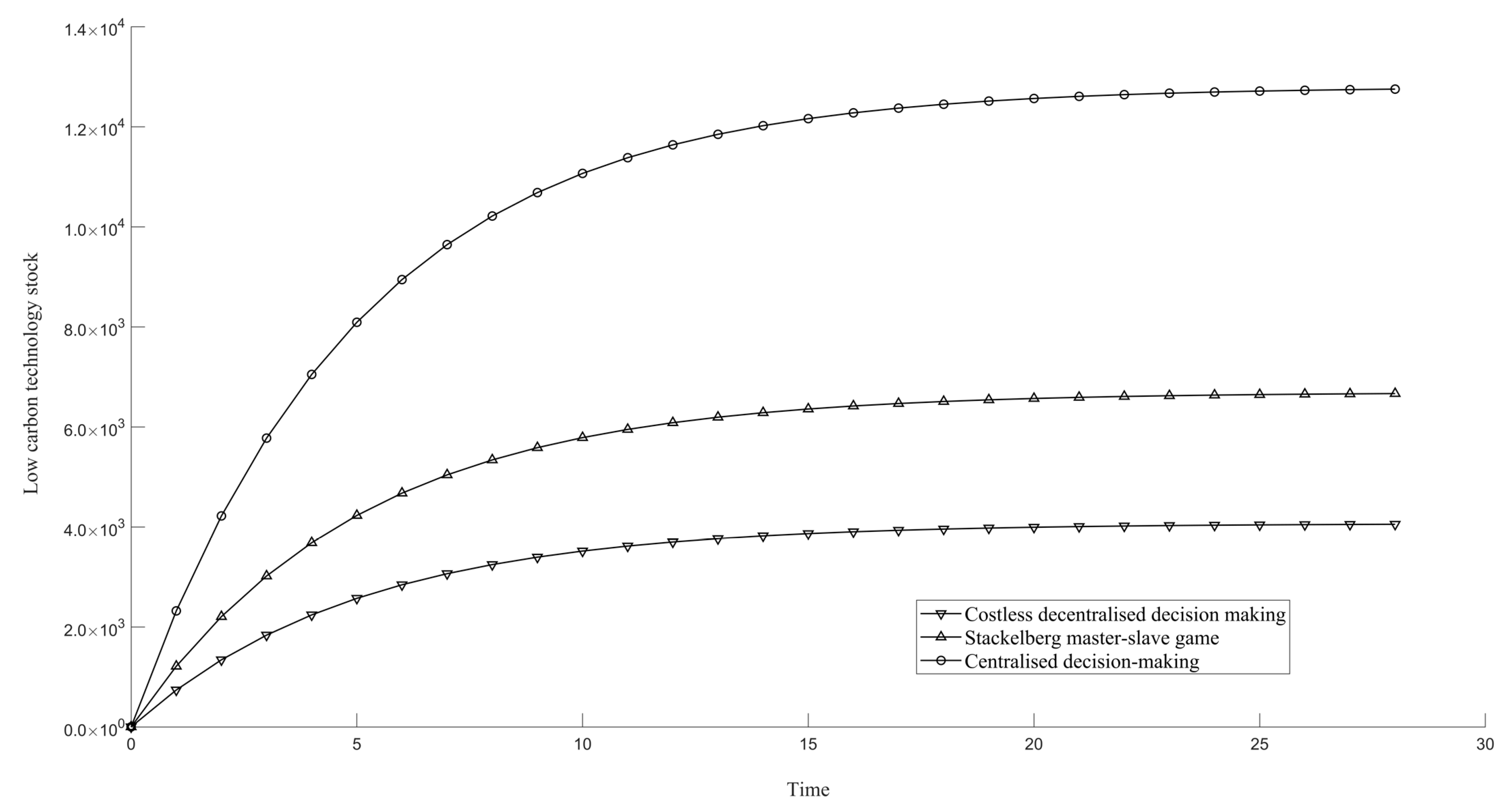
Figure 2 depicts the total regional low-carbon innovative technology stock in different decision-making scenarios. Through comparison, it is found that the LCT in other methods will gradually increase with time and eventually become stable, proving that LCT can be regulated and increased by specific means. At the same time, the LCT in centralized decision making is much higher than in decentralized decision making, which shows that centralized decision making is the ideal scenario for LCT innovation.

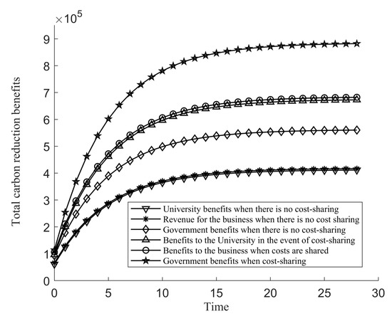
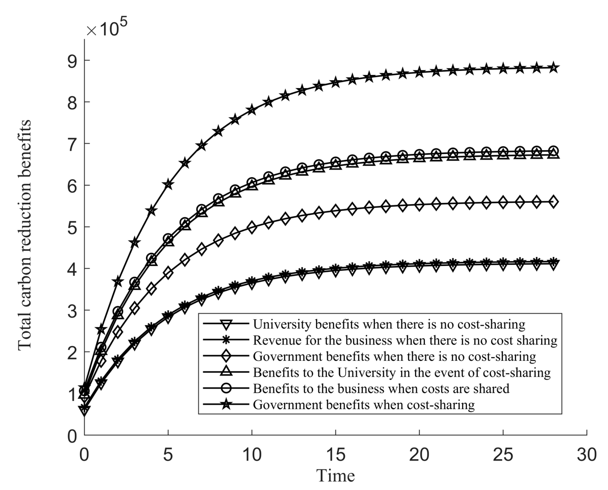
Figure 3 depicts the benefit comparison of the three parties in decentralized decision making. It can be seen that the cost-sharing contract can realize the Pareto improvement of the benefits of the three parties, and the improvement effect of the local government is particularly remarkable. Through the cost-sharing arrangement, the innovation will consist of LCT in universities, traditional enterprises can be stimulated, and the overall benefits can be improved. Promoting LCT can bring certain environmental benefits to the government, thus enhancing the interests of the three parties.

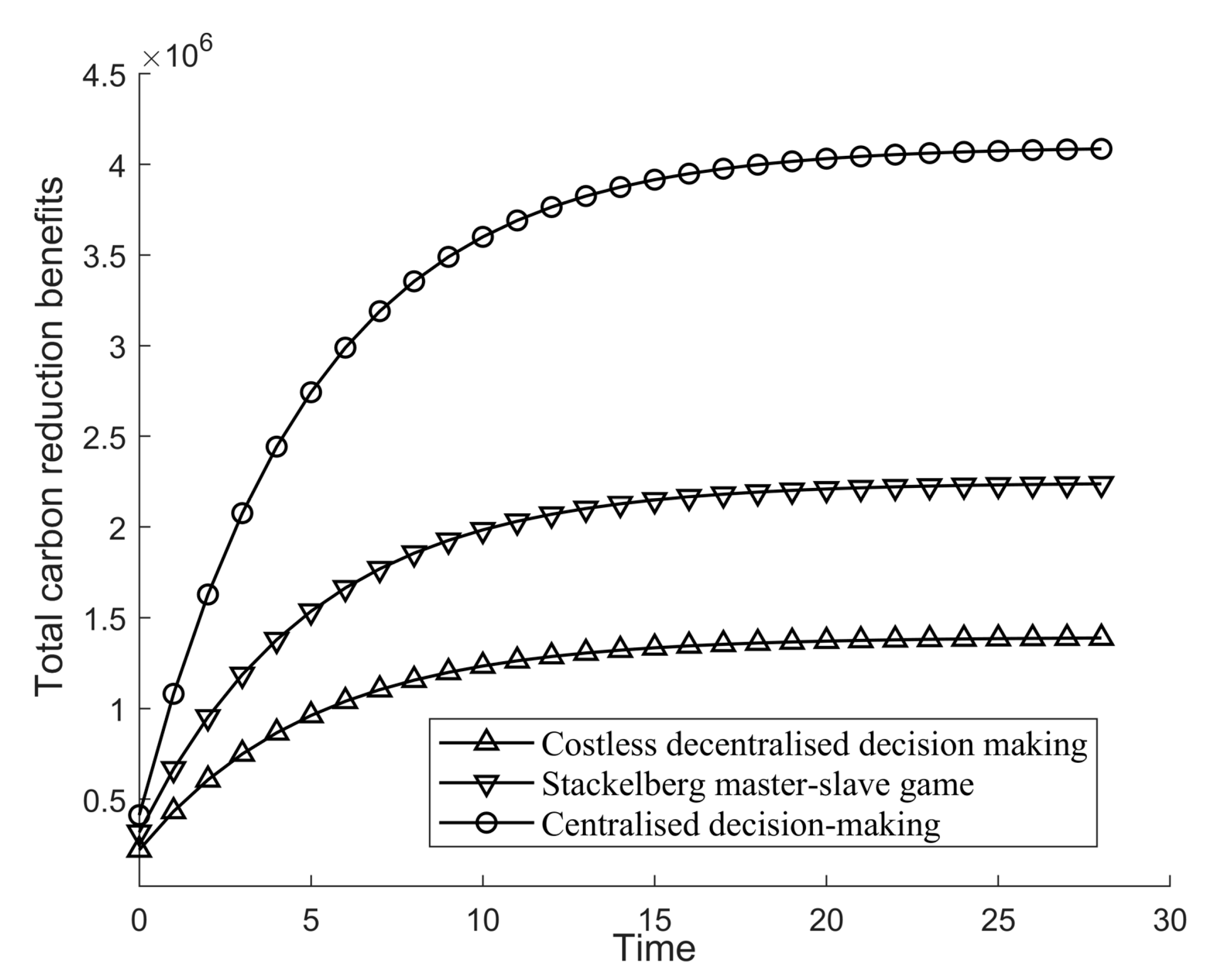
Figure 4 describes the comparison of total regional benefits under three-game scenarios. It can be known that the decentralized decision-making game of cost-sharing is not as significant as the centralized decision making in improving the natural gift, which is because the decentralized decision making game of cost-sharing pays attention to the redistribution of benefits and does not correctly consider how to make the benefits of carbon emission reduction more significant.

Cooperative decision making among universities, traditional enterprises, and local government can realize the advantages shared among the three parties and stimulate the synergistic effect of carbon emission reduction. Such cooperation can enhance the interests and efforts of the three parties.

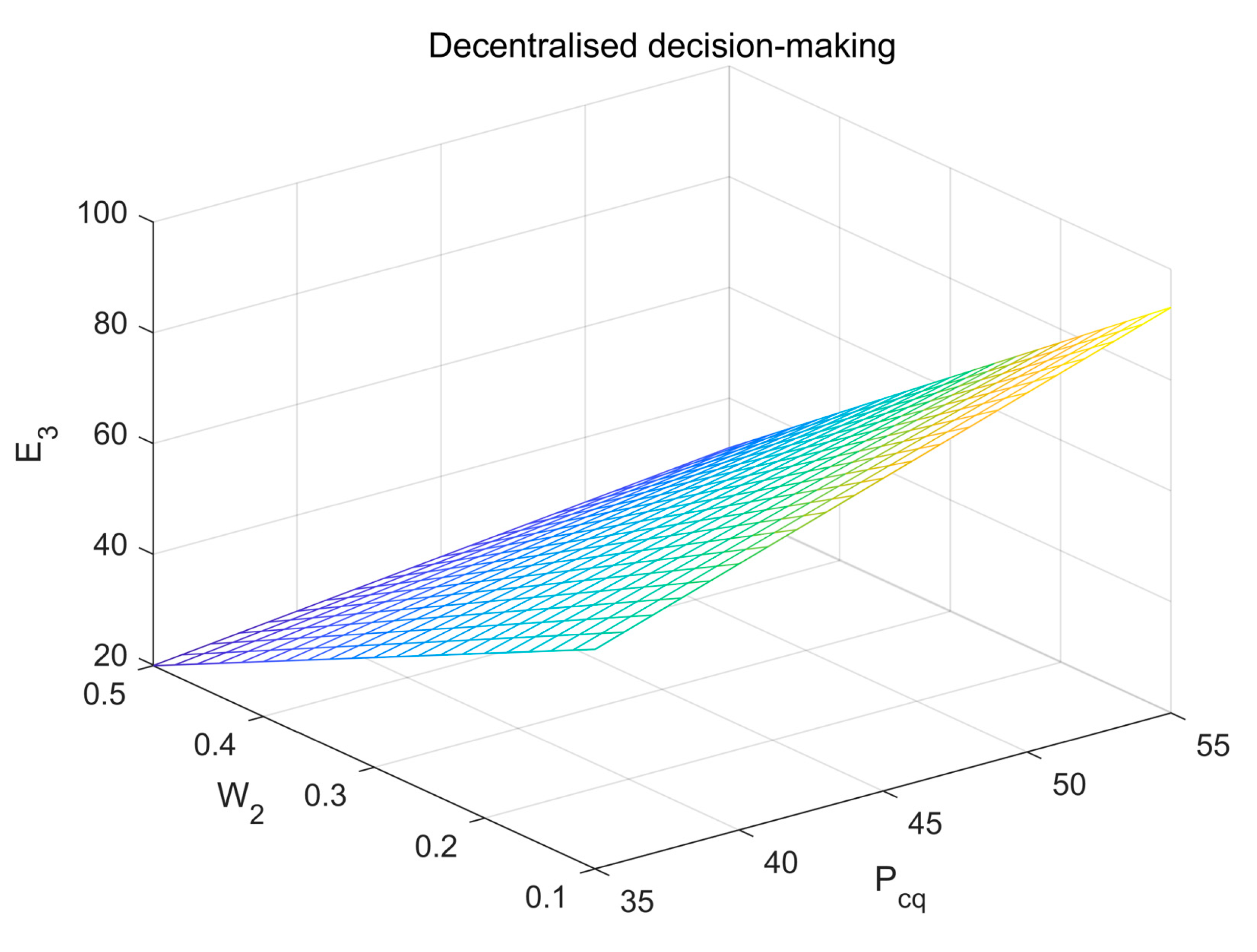
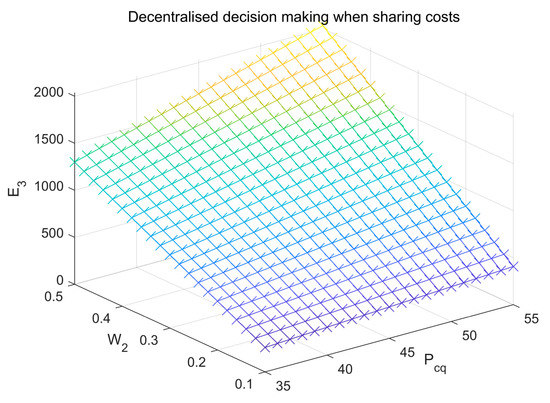
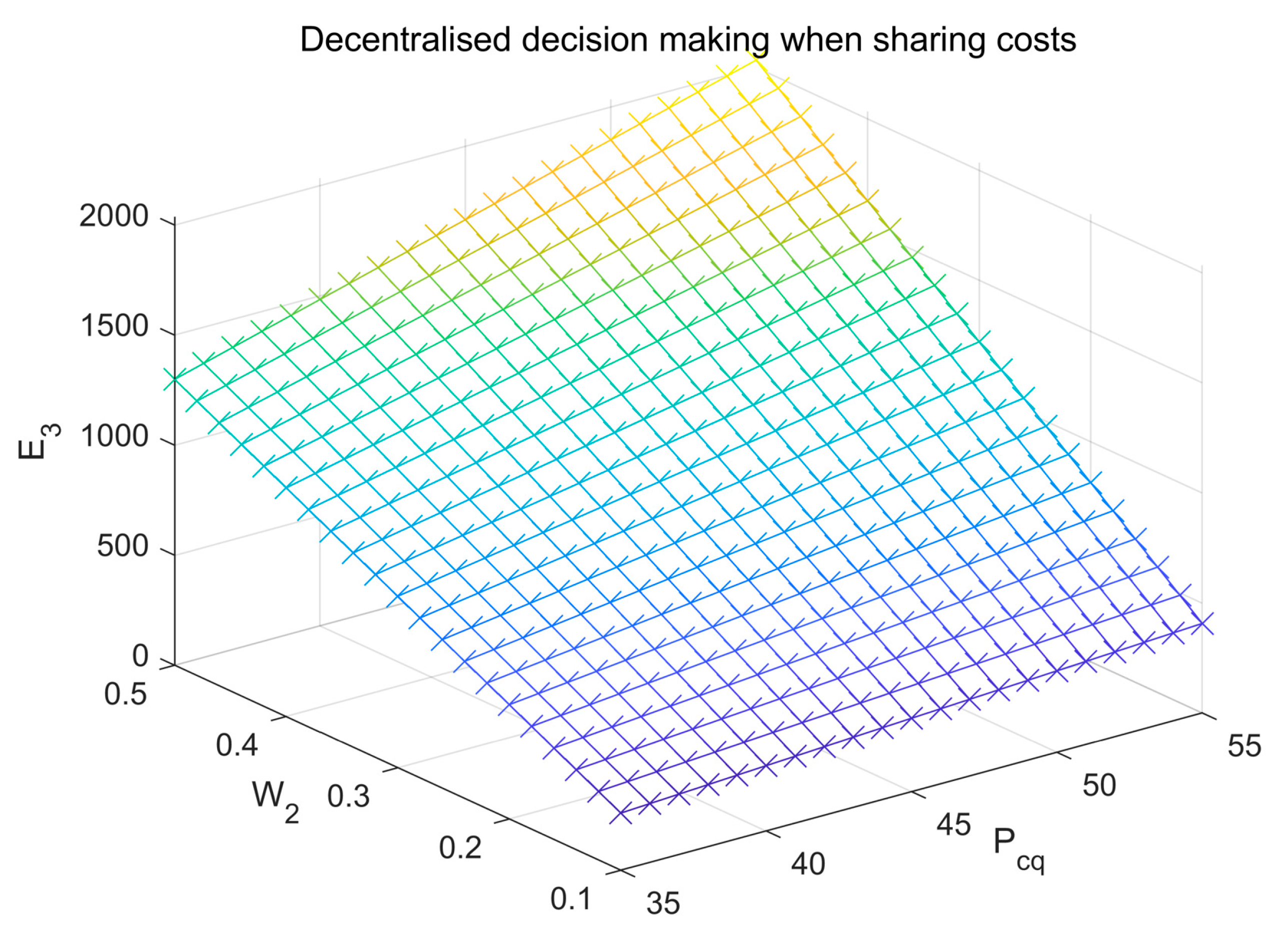
5.2. Sensitivity Analysis in Decentralized Decision Making

Considering the influence of carbon transaction price $P_{cq}$ and profit distribution ratio $W_2$ on the government’s best environmental governance efforts and the traditional enterprises’ best LCT innovation efforts, the results are as follows:

As can be seen in Figure 5 and Figure 6, the adoption of cost-sharing contracts does not affect the level of the government effort to govern the environment. As the carbon trading price and the self-benefit sharing ratio increase, the story of the government’s effort to control the setting and the level of low-carbon innovation effort by traditional enterprises will also increase. The fact that the trading price is determined by the market and the benefit-sharing ratio is negotiated between the government, universities, and traditional enterprises means that government departments can regulate the level of low-carbon innovation efforts by traditional enterprises through cost-sharing contracts, in addition to holding the price of carbon credits and allowances. In addition, China’s carbon trading tax rate is still in its implementation phase. The central government can change the tax rate and benefit-sharing ratio of carbon trading to motivate the three parties in LCT innovation activities.

5.3. Sensitivity Analysis in Centralized Decision Making

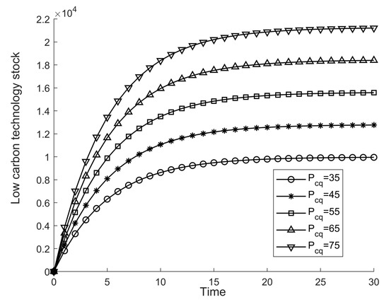
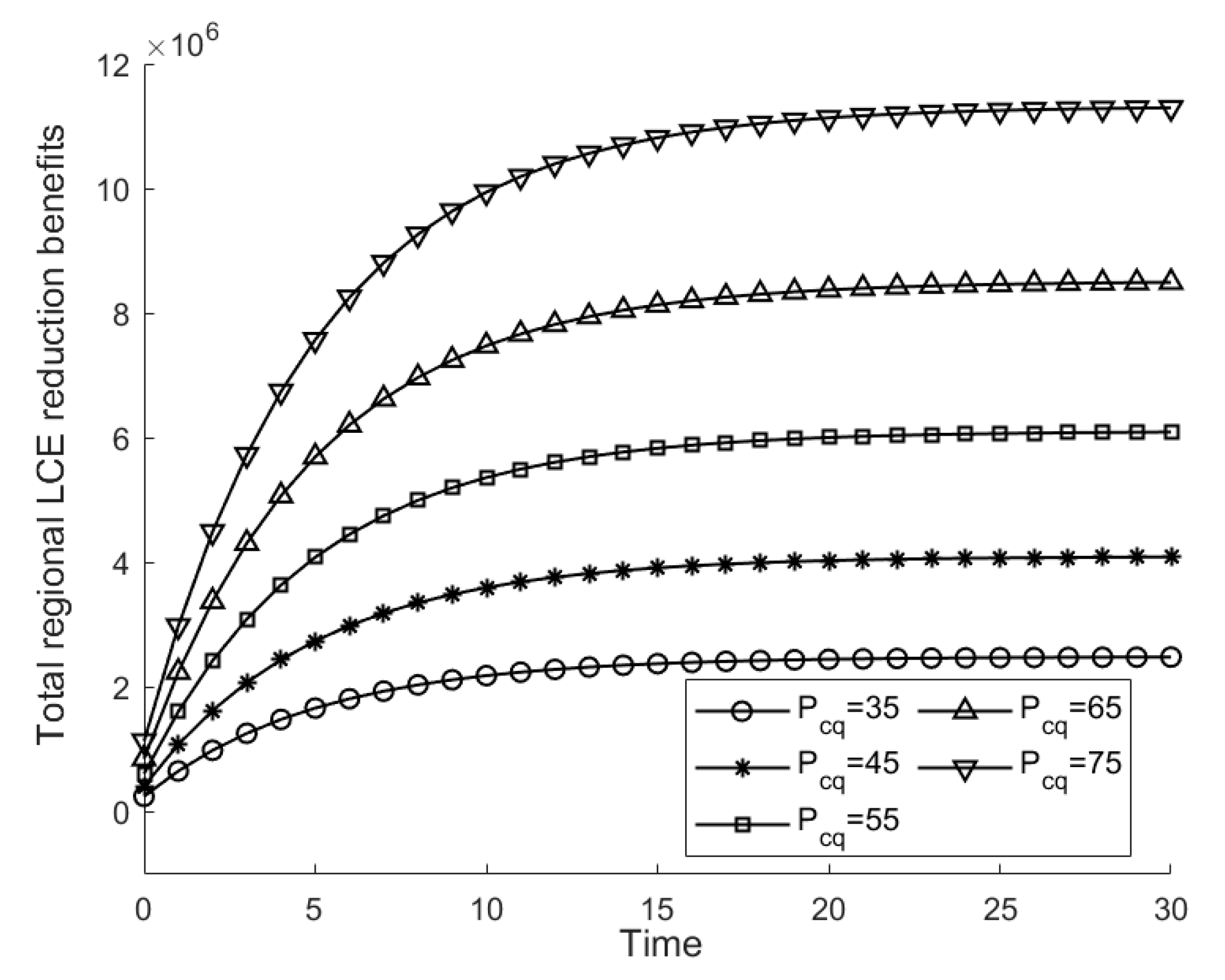
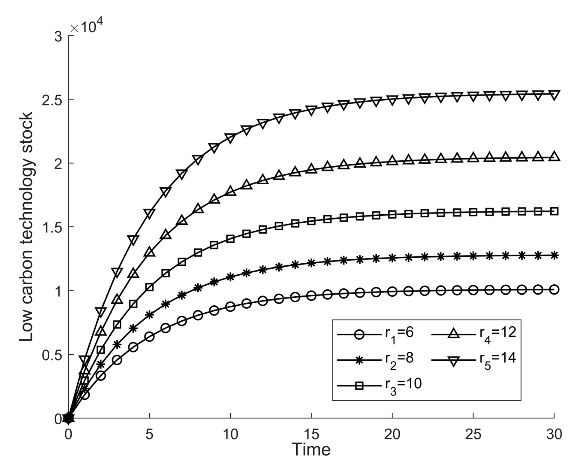
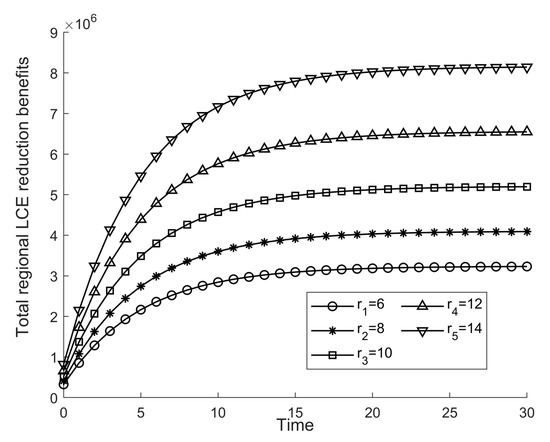
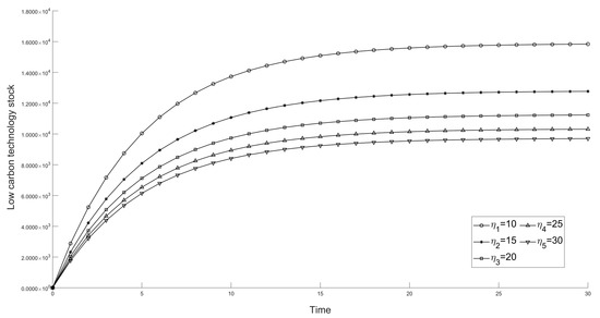
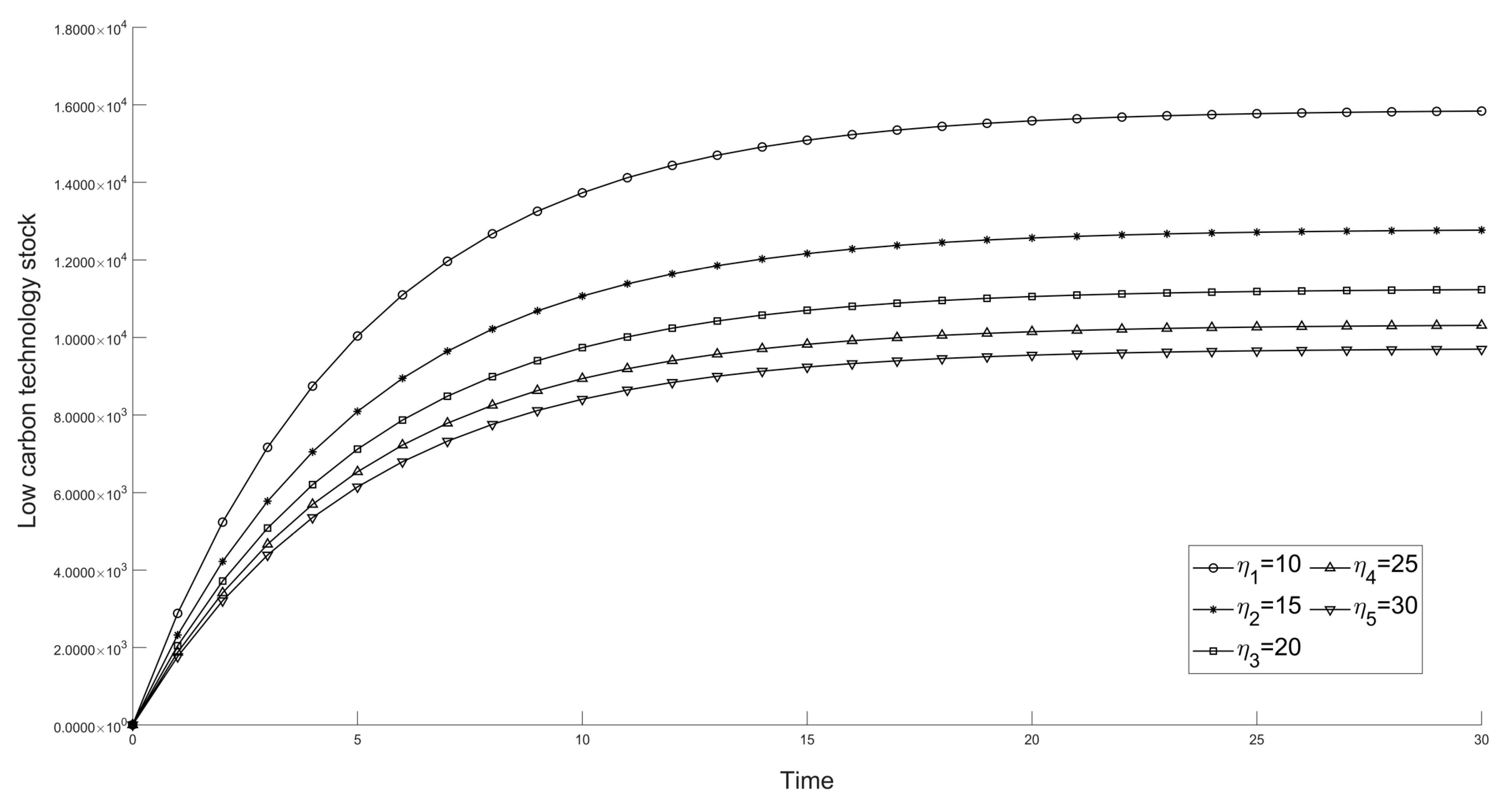
From the above analysis, it can be seen that the LCT stock and total system benefits at the time of centralized decision making are the most desirable scenarios, so the sensitivity analysis that follows will focus mainly on the impact of relevant parameters on the LCT stock and benefits at the time of centralized decision making, considering the brevity of the thesis, focusing on representative parameters including the carbon trading price, the university, the coefficient of the impact of the level of LCT innovation on the stock of LCT, the effort cost coefficient of LCT innovation in universities, the decline rate of the supply of carbon-reducing technologies, and the total profit distribution ratio. The remaining parameters, such as the effort cost coefficient of government participation in environmental governance, are similar to the conclusions of the analysis of the above parameters or will not change anytime soon and will not be repeated.

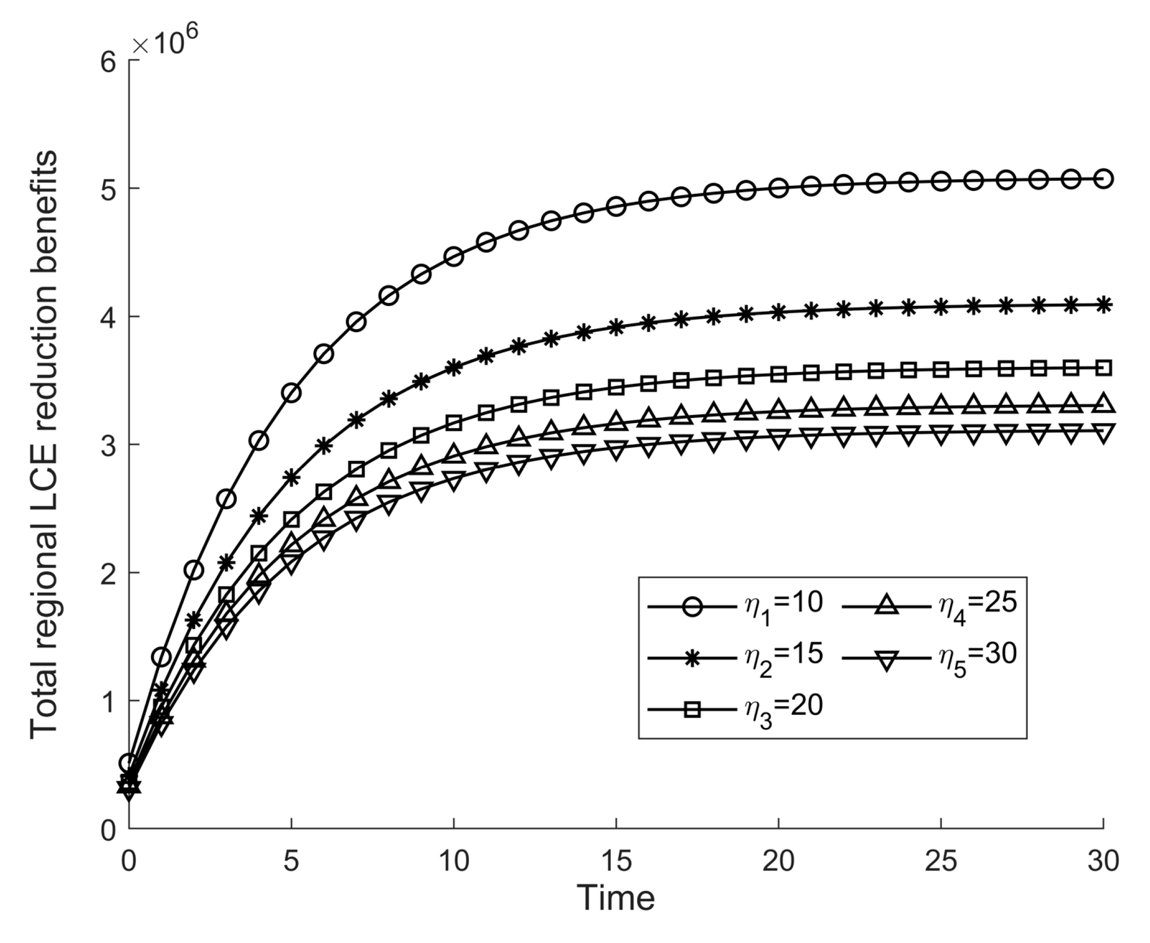
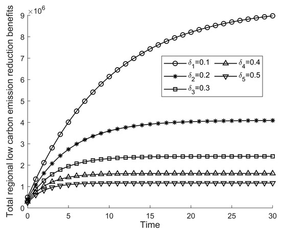
From Figure 7, Figure 8, Figure 9 and Figure 10, it can be seen that parameters such as carbon trading price positively affect regional LCT stock and total regional profit. The result of LCT stock is more prominent. Promoting LCT innovation is an excellent way to achieve green and quiet carbon development. To carry out practical LCT innovation, local governments can provide relevant guidance and assistance to achieve more incredible LCT innovation with less expenditure.

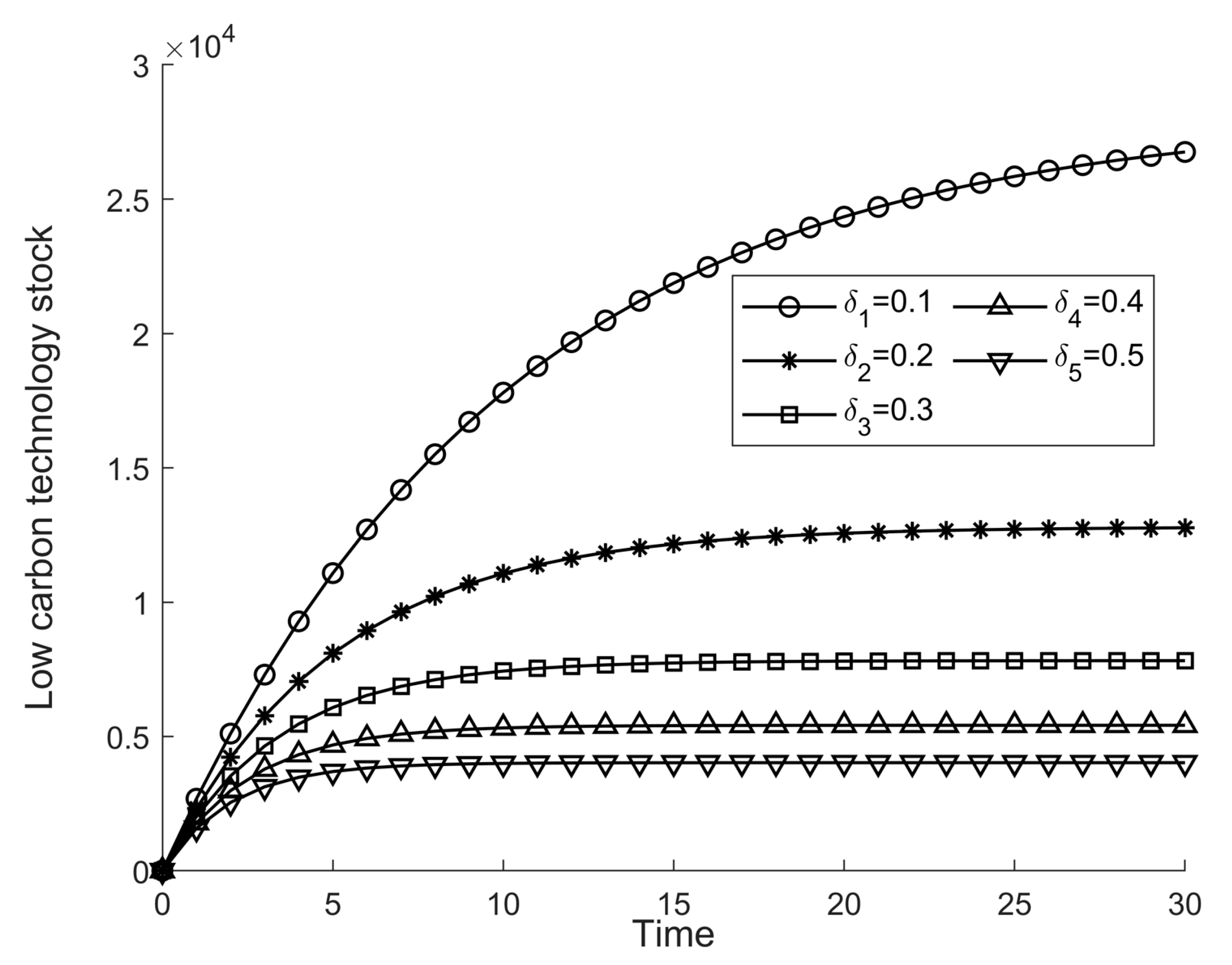
From Figure 11, Figure 12, Figure 13 and Figure 14, it can be seen that ${\eta }_1$ and $\delta$ have an inverse effect on the stock of LCT and total regional profits. When the investment cost of LCT innovation by universities and traditional enterprises is higher, the whole restricted stock of LCT and total profits are less susceptible; at the same time, the higher the rate of decline, the faster the entire regional stock of LCT, and total profits will also decline, which is caused by the ageing of equipment and by equipment replacement.

6. Research Findings and Conclusions

This paper investigates the decision-making problem of universities, traditional enterprises, and local governments in determining their optimal levels of effort in an LCT innovation system under a carbon trading policy. Based on relevant assumptions, differential game models with cost-sharing decentralized decision making, cost-less decentralized decision making, and centralized decision making are constructed to obtain the optimal trajectories of the optimal strategies, optimal LCT stocks, and maximum regional profits for universities, traditional enterprises, and local government, respectively.

First, the analysis compares the trajectory of total regional benefits, the rotation of total regional LCT stock, and the profit trajectory of universities, traditional enterprises, and local governments before and after cost-sharing under the three decision scenarios, and the following conclusions are obtained: (1) in general, the total regional benefits and the total regional LCT stock will be higher in centralized decision making than in decentralized decision making, reaching Pareto optimality; (2) the use of cost-sharing contracts can achieve a Pareto increase in the benefits of the three parties, and the increase is particularly significant for local government. Through cost-sharing contracts, the willingness of universities and traditional enterprises to innovate in LCT can be stimulated, and the total benefits can be increased; due to the improvement in LCT, certain environmental benefits can be brought to the government, thus enhancing the interests of the three parties. Through this study, government planners should determine the optimal benefit-sharing coefficient based on the interests of the three parties, with enterprises and universities being able to gain more from the benefits. Local governments can achieve more significant environmental benefits with less subsidy expenditure.

Secondly, by analyzing the impact of carbon trading policies on the optimal level of effort of universities, traditional enterprises, and local governments, it can be learned that (1) the central government can change the level of effort of universities, traditional enterprises, and local governments by changing the carbon trading tax rate and regulating the price of carbon trading; (2) cost-sharing contracts can enhance the level of effort of universities and traditional enterprises; (3) cost-sharing contracts do not affect the level of effort of local governments’ efforts to govern the environment.

Then, by analyzing the effects of the relevant parameters on the stock of LCT and total benefits under the centralized decision-making scenario, the following conclusions were obtained: (1) the parameters have positive effects on the stock of LCT and the total benefits of the region; (2) parameters such as and hurt the stock of LCT and the total regional benefits.

Finally, the paper yields the following management insights: (1) The central government can regulate carbon trading prices and carbon trading tax rates, and local governments can adopt cost-sharing contracts to improve the level of LCT in low-carbon innovation systems, thereby achieving green and low-carbon production. (2) A reasonable ratio of benefit distribution can promote the maximization of benefits for all three parties and optimize the regional stock of low-carbon technologies. The construction of a tripartite system of cooperative development led by the local government, as concluded above, will result in an optimum level of effort by the local government, enterprises, and universities in a cooperative situation. (3) Subsidies for scientific and technological innovation should be increased to reduce the cost loss of abatement equipment as soon as possible and increase the level of effort of universities and traditional enterprises in low-carbon innovation. At this stage, China’s subsidy system is still not perfect, and local governments can further increase funding subsidies to improve the LCT to achieve economic growth and environmental protection at the same time.

In summary, previous studies have only considered the costs associated with the operation of enterprises without considering the direct economic losses caused by carbon emissions [8,9]. Most existing studies [10,11] have only studied the cooperative innovation system between government and enterprises without considering the role of technology suppliers (universities) addressed in this paper. In this paper, we propose three different models of government–industry–research cooperation using the differential game model and analyze the parameters of maximum benefit and optimal LCT level of university–enterprise–local government in these three models. Then, the author uses accurate data simulation to verify the proposed conclusions. This paper is a new application of differential game theory, which enriches the existing theoretical literature on LCT innovation and differential game theory and not only highlights the importance of LCT but also proposes a more specific subsidy model to improve the LCT level. This is the outstanding contribution of this paper.

There are some limitations to this study. First, the model in this paper is constructed only under a carbon trading system. In practice, dealing with the carbon trading and tax systems may be necessary. Secondly, this work is based on numerical simulation and model derivation, which should be supplemented with case studies or empirical econometric analysis; in the future more research using multiple case studies and incorporate real-life business situations. Finally, solving the differential response model assumes that specific parameters do not change over time, and there is a particular gap with reality. A fully dynamic model needs to be refined in future research, which are the directions for future research.

References

- Pu, X.; Song, Z.; Han, G. Competition among Supply Chains and Governmental Policy: Considering Consumers’ Low-Carbon Preference. Int. J. Environ. Res. Public Health 2018, 15, 1985. [Google Scholar] [CrossRef] [PubMed] [Green Version]
- Birkenberg, A.; Narjes, M.E.; Weinmann, B.; Birner, R. The potential of carbon neutral labeling to engage coffee consumers in climate change mitigation. J. Clean. Prod. 2020, 278, 123621. [Google Scholar] [CrossRef]
- Causone, F.; Tatti, A.; Alongi, A. From Nearly Zero Energy to Carbon-Neutral: Case Study of a Hospitality Building. Appl. Sci. 2021, 11, 10148. [Google Scholar] [CrossRef]
- Ma, J.; Hu, Q.; Shen, W.; Wei, X. Does the Low-Carbon City Pilot Policy Promote Green Technology Innovation? Based on Green Patent Data of Chinese A-Share Listed Companies. Int. J. Environ. Res. Public Health 2021, 18, 3695. [Google Scholar] [CrossRef] [PubMed]
- Chen, X.; Gong, W.; Wang, F. Managing Carbon Footprints under the Trade Credit. Sustainability 2017, 9, 1235. [Google Scholar] [CrossRef] [Green Version]
- Xian, Y.; Wang, K.; Wei, Y.-M.; Huang, Z. Would China’s power industry benefit from nationwide carbon emission permit trading? An optimization model-based ex post analysis on abatement cost savings. Appl. Energy 2018, 235, 978–986. [Google Scholar] [CrossRef] [Green Version]
- Luo, W.; Zhang, Y.; Gao, Y.; Liu, Y.; Shi, C.; Wang, Y. Life cycle carbon cost of buildings under carbon trading and carbon tax system in China. Sustain. Cities Soc. 2020, 66, 102509. [Google Scholar] [CrossRef]
- Shen, L.; Tao, F.; Wang, S. Multi-Depot Open Vehicle Routing Problem with Time Windows Based on Carbon Trading. Int. J. Environ. Res. Public Health 2018, 15, 2025. [Google Scholar] [CrossRef] [Green Version]
- Song, X.; Jiang, X.; Zhang, X.; Liu, J. Analysis, Evaluation and Optimization Strategy of China Thermal Power Enterprises’ Business Performance Considering Environmental Costs under the Background of Carbon Trading. Sustainability 2018, 10, 2006. [Google Scholar] [CrossRef]
- Wu, L. How can carbon trading price distortion be corrected? An empirical study from China’s carbon trading pilot markets. Environ. Sci. Pollut. Res. 2021, 28, 66253–66271. [Google Scholar] [CrossRef] [PubMed]
- Lin, B.; Ge, J. Valued forest carbon sinks: How much emissions abatement costs could be reduced in China. J. Clean. Prod. 2019, 224, 455–464. [Google Scholar] [CrossRef]
- Hong, S.H. Determinants of Selection of R&D Cooperation Partners: Insights from Korea. Sustainability 2021, 13, 9637. [Google Scholar] [CrossRef]
- Song, Y.W.; Zhang, J.R.; Song, Y.K. Can industry-university-research collaborative innovation efficiency reduce carbon emissions? Technol. Forecast Soc. 2020, 157, 120094. [Google Scholar] [CrossRef]
- Zhao, D.D.; Zhou, H. Livelihoods, Technological Constraints, and Low-Carbon Agricultural Technology Preferences of Farmers: Analytical Frameworks of Technology Adoption and Farmer Livelihoods. Int. J. Environ. Res. Public Health 2021, 18, 13364. [Google Scholar] [CrossRef]
- Yan, Z.; Yi, L.; Du, K.; Yang, Z. Impacts of Low-Carbon Innovation and Its Heterogeneous Components on CO2 Emissions. Sustainability 2017, 9, 548. [Google Scholar] [CrossRef] [Green Version]
- Ma, C.S.; Hou, B.; Yuan, T.T. Low-Carbon Manufacturing Decisions Considering Carbon Emission Trading and Green Technology Input. Environ. Eng. Manag. J. 2020, 19, 1593–1604. [Google Scholar]
- Ding, S.T.; Zhang, M.; Song, Y. Exploring China’s carbon emissions peak for different carbon tax scenarios. Energy Policy 2019, 129, 1245–1252. [Google Scholar] [CrossRef]
- Suk, S.; Lee, S.-Y.; Jeong, Y.S. A survey on the impediments to low carbon technology investment of the petrochemical industry in Korea. J. Clean. Prod. 2016, 133, 576–588. [Google Scholar] [CrossRef]
- Sohail, M.T.; Ehsan, M.; Riaz, S.; Elkaeed, E.B.; Awwad, N.S.; Ibrahium, H.A. Investigating the Drinking Water Quality and Associated Health Risks in Metropolis Area of Pakistan. Front. Mater. 2022, 9, 864254. [Google Scholar] [CrossRef]
- Si, F.; Yan, Z.; Wang, J.; Dai, D. Dynamic Analysis of Duopoly Price Game Based on Low-Carbon Technology Sharing. Math. Probl. Eng. 2020, 2020, 3832571. [Google Scholar] [CrossRef]
- Wang, H.; He, Y.; Ding, Q. The impact of network externalities and altruistic preferences on carbon emission reduction of low carbon supply chain. Environ. Sci. Pollut. Res. 2022, 1–18. [Google Scholar] [CrossRef] [PubMed]
- Wang, M.Y.; Li, Y.; Li, M.; Shi, W.; Quan, S. Will carbon tax affect the strategy and performance of low-carbon technology sharing between enterprises? J. Clean. Prod. 2019, 210, 724–737. [Google Scholar] [CrossRef]
- Wei, J.; Wang, C. Improving interaction mechanism of carbon reduction technology innovation between supply chain enterprises and government by means of differential game. J. Clean. Prod. 2021, 296, 126578. [Google Scholar] [CrossRef]
- Deng, Y.; You, D.; Zhang, Y. Research on improvement strategies for low-carbon technology innovation based on a differential game: The perspective of tax competition. Sustain. Prod. Consum. 2021, 26, 1046–1061. [Google Scholar] [CrossRef]
- Ding, Y.; Wang, Y. The research on control mechanism to environmental regulation and high-tech enterprises technology innovation. In Proceedings of the 2014 International Conference on Management Science & Engineering 21th Annual Conference Proceedings, Helsinki, Finland, 17–19 August 2014; pp. 1720–1724. [Google Scholar]
- Kneller, R.; Manderson, E. Environmental regulations and innovation activity in UK manufacturing industries. Resour. Energy Econ. 2012, 34, 211–235. [Google Scholar] [CrossRef]
- Zhang, J.; Liang, G.; Feng, T.; Yuan, C.; Jiang, W. Green innovation to respond to environmental regulation: How external knowledge adoption and green absorptive capacity matter? Bus. Strategy Environ. 2020, 29, 39–53. [Google Scholar] [CrossRef]
- Yu-Hong, C.; Jian-Xin, Y.; Hu-Chen, L. Optimal Environmental Regulation Intensity of Manufacturing Technology Innovation in View of Pollution Heterogeneity. Sustainability 2017, 9, 1240. [Google Scholar]
- Liu, X.B.; Gao, X. A survey analysis of low carbon technology diffusion in China’s iron & steel industry. J. Clean. Prod. 2016, 129, 88–101. [Google Scholar]
- Wang, Y.; Shen, N. Environmental regulation and environment productivity: The case of China. Renew. Sustain. Energy Rev. 2016, 62, 758–766. [Google Scholar] [CrossRef]
- Day, R. Low carbon thermal technologies in an ageing society—What are the issues? Energy Policy 2015, 84, 250–256. [Google Scholar] [CrossRef]
- Wu, C.B.; Liu, P.; Xu, X. An evolutionary analysis of low-carbon strategies based on the government–enterprise game in the complex network context. J. Clean. Prod. 2017, 141, 168–179. [Google Scholar] [CrossRef]
- Zhang, C.T.; Liu, L.P. Research on coordination mechanism in three-level green supply chain under non-cooperative game. Appl. Math. Modell. 2013, 37, 3369–3379. [Google Scholar] [CrossRef]
- Sheng, J.; Zhou, W.; Zhu, B. The coordination of stakeholder interests in environmental regulation: Lessons from China’s environmental regulation policies from the perspective of the evolutionary game theory. J. Clean. Prod. 2019, 249, 119385. [Google Scholar] [CrossRef]
- Xin, B.; Sun, M. A differential oligopoly game for optimal production planning and water savings. Eur. J. Oper. Res. 2018, 269, 206–217. [Google Scholar] [CrossRef]
- Liu, L.; Wang, Z.; Li, X.; Liu, Y.; Zhang, Z. An evolutionary analysis of low-carbon technology investment strategies based on the manufacturer-supplier matching game under government regulations. Environ. Sci. Pollut. Res. 2022, 29, 44597–44617. [Google Scholar] [CrossRef]
- Zhang, W.; Zhao, S.; Wan, X. Industrial digital transformation strategies based on differential games. Appl. Math. Model. 2021, 98, 90–108. [Google Scholar] [CrossRef]
- El Ouardighi, F.; Kogan, K. Dynamic conformance and design quality in a supply chain: An assessment of contracts’ coordinating power. Ann. Oper. Res. 2013, 211, 137–166. [Google Scholar] [CrossRef]
- Hong, J.; Huang, P. Research on quality coordination in supply chain based on differential game. Chin. J. Manag. Sci. 2016, 24, 100–107. [Google Scholar]
- Wang, L.; Shi, H.-B.; Yu, S.; Li, H.; Liu, L.; Bi, Z.; Fu, L. An application of enterprise systems in quality management of products. Inf. Technol. Manag. 2012, 13, 389–402. [Google Scholar] [CrossRef]
- Tse, Y.K.; Tan, K.H. Managing product quality risk in a multi-tier global supply chain. Int. J. Prod. Res. 2011, 49, 139–158. [Google Scholar] [CrossRef]
- Guo, F.; Wang, J.; Liu, D.; Song, Y. Evolutionary Process of Promoting Construction Safety Education to Avoid Construction Safety Accidents in China. Int. J. Environ. Res. Public Health 2021, 18, 10392. [Google Scholar] [CrossRef] [PubMed]
- Song, Y.; Wang, J.; Liu, D.; Huangfu, Y.; Guo, F.; Liu, Y. The Influence of Government’s Economic Management Strategies on the Prefabricated Buildings Promoting Policies: Analysis of Quadripartite Evolutionary Game. Buildings 2021, 11, 444. [Google Scholar] [CrossRef]
- Guo, F.; Wang, J.; Song, Y. How to promote sustainable development of construction and demolition waste recycling systems: Production subsidies or consumption subsidies? Sustain. Prod. Consum. 2022, 32, 407–423. [Google Scholar] [CrossRef]
Publisher’s Note: MDPI stays neutral with regard to jurisdictional claims in published maps and institutional affiliations. |
© 2022 by the authors. Licensee MDPI, Basel, Switzerland. This article is an open access article distributed under the terms and conditions of the Creative Commons Attribution (CC BY) license (https://creativecommons.org/licenses/by/4.0/).