Crop Diversification in South Asia: A Panel Regression Approach

Abstract

The South Asian agricultural sector has experienced vigorous growth and structural transformation over the last few decades, albeit differently across the region. This study examines the crop diversification status and various determinants, such as socioeconomic (per capita gross domestic product, population, arable land, and cropland), soil/agronomic (root zone moisture), agricultural inputs (fertilizer and pesticide consumption), the productivity of food and non-food crops, international trade, and climate (maximum and minimum temperature and rainfall) factors. The share of cereals has decreased in most countries, but they continue to dominate South Asian agriculture. The area under high-value crops in India has increased significantly, replacing the area under cereal cultivation during the study period. Similar results were seen in the Maldives, where vegetables replaced oilseeds. The Hausman model test suggested a random-effects model for analyzing the determinants. All the determinants considered in the study explain 69 percent of the variation in the crop diversification index. The crop diversification in South Asia was influenced by per capita gross domestic product (G.D.P.), minimum temperature, pesticide consumption, food crop yield index, and non-food crop yield index during the study period. Cropland percentage and population, on the other hand, reduce crop diversification. The price factor contributed more than half to agricultural growth. It remained the primary source of growth in all South Asian countries, followed by yield, which is identified as the second most crucial factor. The contribution of crop diversification to agricultural growth has been declining over time.

1. Introduction

Agriculture growth is both essential and sufficient to initiate the structural transformation process, which results in agriculture’s contribution to G.D.P. falling from roughly 30% in 1970 to 17% in 2017 [1]. More than a quarter of the developing world’s population lives in South Asia, and approximately 72 percent live in rural areas. However, in South Asia, the majority (94%) of suitable agricultural land has already been leaving no scope to expand [2]. South Asia’s area under annual and permanent crops is expected to be 213 million ha (nearly half of total land area) by 2030, with only a minor increase [3]. Furthermore, new land area is primarily derived from pasture and forest land, implying substantial investments and some foregone development [4]. Since the late 1980s, South Asian economies have been undergoing economic reforms. Trade liberalization is being gradually incorporated into their policy framework. However, the ongoing globalization of agriculture has presented these countries’ agricultural sectors with new challenges and opportunities.

Food security remains a critical issue in the subcontinent. Government policy continues to be obsessed with cereal self-sufficiency, which presumably contributes to a large portion of land being allocated to cereal crops. Countries, such as Bangladesh, India, and Sri Lanka, have achieved national food security, but the focus remains on increasing rice and wheat production. Nations with food grain production deficits, such as Bhutan, Nepal, and Pakistan, are making serious efforts to increase production [5]. The current situation in the South Asian region raises severe concerns about overexploitation of natural resources, rural employment, the livelihood of agriculturist farm households, food security, and sustainability.

Crop diversification has enormous potential as an economic driver within the agricultural sector, which could be critical in meeting the challenges discussed earlier in this study. It has also become vital for achieving higher output growth, increasing farm income, creating jobs, conserving precious soil and water resources, consumer preferences for high-value, nutrient-dense foods, rural livelihood, sustainable use of natural resources, and poverty alleviation [6,7,8,9,10,11,12]. It can be influenced by socioeconomic, soil and agronomic, agricultural inputs, productivity, international trade, and climatic factors, all considered in this study.

The South Asian developing region is characterized by limited access to financial and technological resources, which must be addressed to achieve quicker, more efficient, and sustainable agricultural expansion and accelerate the pace of structural transformation. The current research focuses on cropping pattern dynamics, agricultural diversification, and various determinants, such as socioeconomic, soil/agronomic, agricultural inputs, the productivity of food and non-food crops, international trade, and climate factors. There have been many studies on crop diversification in South Asia. However, few studies focus on crop diversification at the country level using a panel regression approach [1], and no study has delineated the determinants of growth. This model gives a quantitative overview of the region and country-specific coefficients in the studied time period. Thus, the study would help identify the determinants of crop diversification and specify region-specific measures to improve crop diversification.

2. Materials and Methods

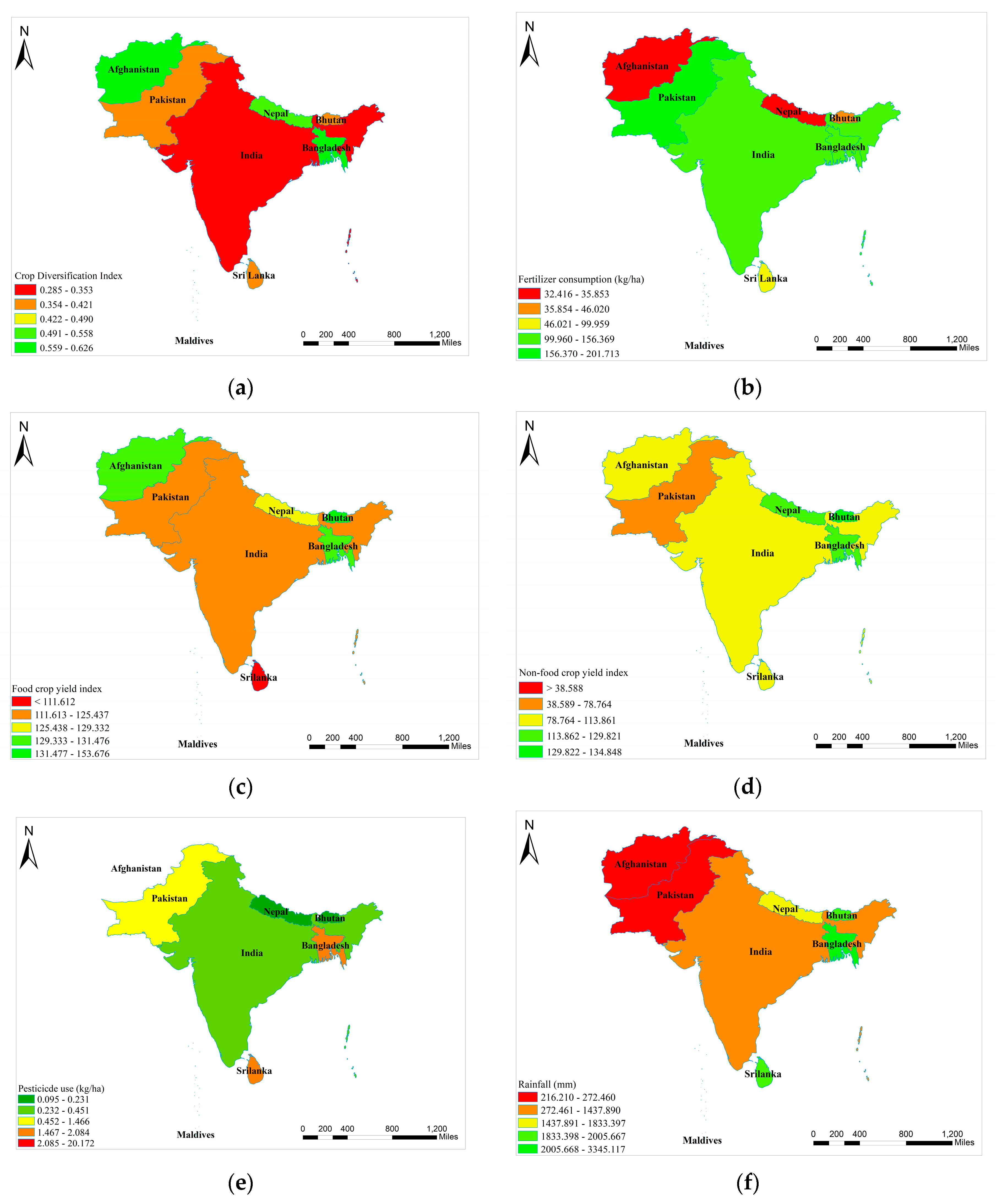
2.1. Study Area

The South Asian region, which includes Afghanistan, Bangladesh, Bhutan, India, Maldives, Nepal, Pakistan, and Sri Lanka, was chosen for the study. The study area comprises of more than twenty-five percent of the world’s population, with 72 percent of them living in rural regions [4].

2.2. The Data

This study uses time series data to examine agricultural transformations in South Asian countries from 1991 to 2020. Food and Agriculture Organisation (FAO) statistics released data on area, production, yield, arable land (ha/person), per capita gross domestic product, population, fertilizer (kg/ha), and pesticide (kg/ha) [2]. Data on exports and imports were obtained from UN Comtrade [13]. In addition, the NASA Power Data Access Viewer, was used to download temperature (maximum and minimum), rainfall, and root zone moisture data for different latitudes and longitudes [14].

2.3. The Analytical Framework

Percentages, averages, and various analytical techniques were used to study the status of South Asian agriculture. The cropping pattern of different South Asian countries was studied using the commodity group’s percentage share.

2.4. Dynamics of Cropping Pattern

The dynamics of cropping patterns were studied in the four following decades, i.e., 1991–2000, 2001–2010, 2011–2020, and 1991–2020, using percent change and compound annual growth rates. The compound growth rates for various variables were calculated by fitting the exponential function to the figures of the area. The power function of the form Y = ae^bt was fitted using the ordinary least square method [15,16]. It was converted into a log-linear function using the logarithmic transformation as follows:

$$\mathrm{Ln}\left(\mathrm{Y}\right)=\mathrm{Ln}\left(\mathrm{a}\right)+\mathrm{bt}$$

(1)

where $\mathrm{Y}$ is the area and t is the time (1991 to 2020).

The following compound annual growth rate (CAGR) formula was used:

$$\mathrm{CAGR}=\mathrm{b}\times 100$$

(2)

The significance of the CAGR was tested by using t-statistics.

2.5. Crop Diversification Index

The entropy index was employed in this study for optimal crop diversification index because, according to Samuelson’s theorem, optimal diversification maximizes the entropy index [15]. When diversification is perfect, the entropy index approaches one, and it approaches zero when it is highly specialized. Crop diversification was examined using the following formula:

$$\mathrm{Crop} \mathrm{Diversification} \mathrm{Index}={{\displaystyle \sum }}_{\mathrm{i}=0}^{\mathrm{N}}{\mathrm{p}}_{\mathrm{i}}\log \frac{1}{{\mathrm{p}}_{\mathrm{i}}}.$$

(3)

where ${\mathrm{p}}_{\mathrm{i}}$ indicates the proportion of the area of the i-th crop, and i goes from 1, 2, …, n [crops].

2.6. Determinants of Crop Diversification

Fixed and random effect models were employed to analyze agricultural diversification drivers at the national level in South Asia. A balanced panel data set was used with equal observations for each country and a sample size of 3360 data points. The Hausman specification test was used to assess the technique’s suitability for data analysis to choose the best model between fixed effect models and random effect models.

According to the Hausman test results, the chi-square value was non-significant, indicating that a random effect model is adequate for examining crop diversification determinants. The specification of variables and their expected signs for diversification are presented in

Table 1. Specification of variables and their expected signs for diversification.

Factors	Indicators	Unit	Expected Sign
Socioeconomic	Per capita GDP	USD	+
	Population	’000 person	-
	Arable land	ha/person	+
	Cropland	Percentage	-
Soil/agronomic	Root zone moisture	Per cent	+
Agricultural inputs	Fertilizer	kg/ha	+
	Pesticide	kg/ha	+
Productivity	Food crop yield index	Per cent	+
	Non-food crop yield index	Per cent	+
International trade	Merchandize index		+
Climate	Temperature (Maximum)	°C	+
	Temperature (Minimum)	°C	+
	Rainfall (mm)	Millimeter	-

.

2.7. Random Effect Model

The random effect model (R.E.M.) implies that the individual-specific coefficient ${\mathsf{\beta }}_{1\mathrm{i}}$ is fixed for each time-in-variant and that ${\mathsf{\beta }}_{1\mathrm{i}}$ is a random variable with a mean value of ${\mathsf{\beta }}_1$ and that the random intercepts change between nations (cross-section units). Dummy variables are used for each country to designate a specific country. It permits heterogeneity or individuality across nations since each has its intercept value. South Asian countries are undergoing different economic reforms and agro-ecological conditions for agriculture crops, so acreage transformation differs by country [11,12]. Therefore, in the current study, the intercept varies across South Asian countries but not over time. Consequently, the random effect model for panel data may be expressed as follows:

$$\begin{array}{ll}\mathrm{E}.\mathrm{D}.\mathrm{I}{.}_{\mathrm{it}}=& {\mathsf{\beta }}_1+{\mathsf{\beta }}_2\mathrm{A}.\mathrm{L}{.}_{\mathrm{it}}+{\mathsf{\beta }}_3\mathrm{G}.\mathrm{D}.\mathrm{P}{.}_{\mathrm{it}}+{\mathsf{\beta }}_4{\mathrm{CL}}_{\mathrm{it}}+{\mathsf{\beta }}_5\mathrm{P}.\mathrm{O}.\mathrm{P}{.}_{\mathrm{it}}+{\mathsf{\beta }}_6{\mathrm{MI}}_{\mathrm{it}}+{\mathsf{\beta }}_7{\mathrm{MAXT}}_{\mathrm{it}}+{\mathsf{\beta }}_8{\mathrm{MIN}}_{\mathrm{it}}+{\mathsf{\beta }}_9\mathrm{R}.\mathrm{Z}.\mathrm{M}{.}_{\mathrm{it}}\\ & +{\mathsf{\beta }}_{10}\mathrm{R}.\mathrm{F}{.}_{\mathrm{it}}+{\mathsf{\beta }}_{11}{\mathrm{F}}_{\mathrm{it}}+{\mathsf{\beta }}_{12}{\mathrm{P}}_{\mathrm{it}}+{\mathsf{\beta }}_{13}{\mathrm{FCYI}}_{\mathrm{it}}+{\mathsf{\beta }}_{14}{\mathrm{NFCYI}}_{\mathrm{it}}+{\mathsf{\beta }}_{15}\mathrm{B}.\mathrm{G}.\mathrm{D}{.}_{\mathrm{it}}+{\mathsf{\beta }}_{16}\mathrm{B}.\mathrm{T}.\mathrm{N}{.}_{\mathrm{it}}+{\mathsf{\beta }}_{17}{\mathrm{IND}}_{\mathrm{it}}\\ & +{\mathsf{\beta }}_{18}{\mathrm{MDV}}_{\mathrm{it}}+{\mathsf{\beta }}_{19}{\mathrm{NPL}}_{\mathrm{it}}+{\mathsf{\beta }}_{20}\mathrm{P}.\mathrm{A}.\mathrm{K}{.}_{\mathrm{it}}+{\mathsf{\beta }}_{19}{\mathrm{LKA}}_{\mathrm{it}}+{\mathrm{w}}_{\mathrm{it}}\end{array}$$

(4)

where ${\mathrm{w}}_{\mathrm{it}}={\mathsf{\epsilon }}_{\mathrm{i}}+{\mathrm{u}}_{\mathrm{it}}$; ${\mathrm{w}}_{\mathrm{it}}$ = composite error term; ${\mathsf{\epsilon }}_{\mathrm{i}}$ = the cross-section or individual-specific error component; ${\mathrm{u}}_{\mathrm{it}}=$ the combined time series and cross-section error component. Annex I presents the specification of variables and their predicted diversification indicators.

2.8. Merchandise Index

The merchandise index measures the magnitude of export market concentration by country of origin. The merchandise index had a positive relationship with the crop diversification index and influenced prices in the domestic market to increase crop diversification.

$$\mathrm{Merchandise} \mathrm{index}=\frac{{\mathrm{X}}_{\mathrm{k}}}{{\mathrm{X}}_{\mathrm{k}}-{\mathrm{M}}_{\mathrm{k}}}$$

(5)

where ${\mathrm{X}}_{\mathrm{k}}$ is the export of the k-th agriculture commodity, and ${\mathrm{M}}_{\mathrm{k}}$ is the import of the k-th agriculture commodity.

2.9. Crop Yield Index

Determining the impact of all the food and non-food crop yields grown at the country’s level, with average yields of the same crop grown in that locality, proves useful in our analysis, as explained below. The index is measured in terms of percentage. The crop yield index computation is discussed below:

$$\mathrm{Production} \mathrm{efficiency} \left(\mathrm{P}.\mathrm{F}{.}_{\mathrm{i}}\right)={\displaystyle \sum }_{\mathrm{i}=0}^{\mathrm{n}}\frac{{\mathrm{AY}}_{\mathrm{i}}}{\mathrm{P}.\mathrm{Y}{.}_{\mathrm{i}}}\times 100$$

(6)

$$\mathrm{Crop} \mathrm{yield} \mathrm{index}=\frac{{{\displaystyle \sum }}_{\mathrm{i}=0}^{\mathrm{n}}\mathrm{P}.\mathrm{F}{.}_{\mathrm{i}}\times {\mathrm{A}}_{\mathrm{i}}}{{{\displaystyle \sum }}_{\mathrm{i}=0}^{\mathrm{n}}{\mathrm{A}}_{\mathrm{i}}}$$

(7)

where $\mathrm{P}.\mathrm{F}{.}_{\mathrm{i}}$ indicates the production efficiency of the i-th crop, ${\mathrm{Y}}_{\mathrm{i}}$ denotes the country’s actual yield of the i-th crop, $\mathrm{P}.\mathrm{Y}{.}_{\mathrm{i}}$ implies the country’s potential yield of the i-th crop, and ${\mathrm{A}}_{\mathrm{i}}$ indicates the country’s area of the i-th crop. Therefore, a high yield index for both food and non-food crops favorably affects the crop diversity index far more than yield improvements in monoculture systems.

2.10. Decomposition of Growth

To examine the share of various sources to agricultural growth, the “growth accounting” method [17,18] is used to dissect the total increase in agriculture. For instance, the rise or change in income from a single crop at two periods in time (or across time) may be broken down into the estimated impact of the area, productivity, and price changes [1,19].

$${\mathrm{R}}_{\mathrm{i}}={\mathrm{X}}_{\mathrm{i}}\times {\mathrm{Y}}_{\mathrm{i}}\times {\mathrm{Z}}_{\mathrm{i}}$$

(8)

where ${\mathrm{X}}_{\mathrm{i}}$ = the area of crop i, ${\mathrm{Y}}_{\mathrm{i}}$ = yield of crop i, and ${\mathrm{Z}}_{\mathrm{i}}$ = actual producer price of i crops, then the ${\mathrm{R}}_{\mathrm{i}}$ from crop i may be stated as follows.

The total revenue is obtained by adding the revenues of n crops:

$$\mathrm{R}={\displaystyle \sum }_{\mathrm{i}=1}^{\mathrm{n}}{\mathrm{X}}_{\mathrm{i}}\times {\mathrm{Y}}_{\mathrm{i}}\times {\mathrm{Z}}_{\mathrm{i}}$$

(9)

A source of adjustment in the decomposition process of total revenue from n crops is crop diversification. For analyzing that, we state that the area under crop i as a proportion of total cropped area, and expressed as, ${\mathrm{M}}_{\mathrm{i}}=\left(\frac{{\mathrm{X}}_{\mathrm{i}}}{{{\displaystyle \sum }}_{\mathrm{i}=0}^{\mathrm{n}}{\mathrm{X}}_{\mathrm{i}}}\right)$, and substitute this in Equation (9):

$$\mathrm{Revenue}=\left({\displaystyle \sum }_{\mathrm{i}=1}^{\mathrm{n}}{\mathrm{M}}_{\mathrm{i}}\times {\mathrm{Y}}_{\mathrm{i}}\times {\mathrm{Z}}_{\mathrm{i}}\right){\displaystyle \sum }_{\mathrm{i}=0}^{\mathrm{n}}{\mathrm{X}}_{\mathrm{i}}$$

(10)

By differencing both the sides of Equation (10) we get the specific contribution of area, yield and price:

$$\partial \mathrm{R}\cong \left({\displaystyle \sum }_{\mathrm{i}=1}^{\mathrm{n}}{\mathrm{M}}_{\mathrm{i}}\times {\mathrm{Y}}_{\mathrm{i}}\times {\mathrm{Z}}_{\mathrm{i}}\right)\partial \left({\displaystyle \sum }_{\mathrm{i}=0}^{\mathrm{n}}{\mathrm{X}}_{\mathrm{i}}\right)+\left({\displaystyle \sum }_{\mathrm{i}=0}^{\mathrm{n}}{\mathrm{X}}_{\mathrm{i}}\right)\partial \left({\displaystyle \sum }_{\mathrm{i}=1}^{\mathrm{n}}{\mathrm{M}}_{\mathrm{i}}\times {\mathrm{Y}}_{\mathrm{i}}\times {\mathrm{Z}}_{\mathrm{i}}\right)$$

(11)

The term $\left({\displaystyle \sum }_{\mathrm{i}=0}^{\mathrm{n}}{\mathrm{X}}_{\mathrm{i}}\right)\partial \left({\displaystyle \sum }_{\mathrm{i}=1}^{\mathrm{n}}{\mathrm{M}}_{\mathrm{i}}\times {\mathrm{Y}}_{\mathrm{i}}\times {\mathrm{Z}}_{\mathrm{i}}\right)$ of Equation (11) can be decomposed as:

$$\partial \mathrm{R}\cong \left({\displaystyle \sum }_{\mathrm{i}=1}^{\mathrm{n}}{\mathrm{M}}_{\mathrm{i}}\times {\mathrm{Y}}_{\mathrm{i}}\times {\mathrm{Z}}_{\mathrm{i}}\right)\partial \left({\displaystyle \sum }_{\mathrm{i}=0}^{\mathrm{n}}{\mathrm{X}}_{\mathrm{i}}\right)+{\displaystyle \sum }_{\mathrm{i}=1}^{\mathrm{n}}\partial \left({\mathrm{M}}_{\mathrm{i}}\times {\mathrm{Y}}_{\mathrm{i}}\times {\mathrm{Z}}_{\mathrm{i}}\right)$$

(12)

Expanding the term ${\displaystyle \sum }_{\mathrm{i}=1}^{\mathrm{n}}\partial \left({\mathrm{M}}_{\mathrm{i}}\times {\mathrm{Y}}_{\mathrm{i}}\times {\mathrm{Z}}_{\mathrm{i}}\right)$ from Equation (12), we can write:

$$\begin{gathered} \partial \mathrm{R}\cong \left({\displaystyle \sum }_{\mathrm{i}=1}^{\mathrm{n}}\mathrm{M}\times {\mathrm{Y}}_{\mathrm{i}}\times {\mathrm{Z}}_{\mathrm{i}}\right)\partial \left({\displaystyle \sum }_{\mathrm{i}=0}^{\mathrm{n}}{\mathrm{X}}_{\mathrm{i}}\right)+\left({\displaystyle \sum }_{\mathrm{i}=0}^{\mathrm{n}}{\mathrm{X}}_{\mathrm{i}}\right){\displaystyle \sum }_{\mathrm{i}=1}^{\mathrm{n}}\left({\mathrm{M}}_{\mathrm{i}}\times {\mathrm{Y}}_{\mathrm{i}}\times \partial {\mathrm{Z}}_{\mathrm{i}}\right) \\ \hspace{1em}\hspace{1em}\hspace{1em}\hspace{1em}\hspace{1em}\hspace{1em}+\left({\displaystyle \sum }_{\mathrm{i}=0}^{\mathrm{n}}{\mathrm{X}}_{\mathrm{i}}\right){\displaystyle \sum }_{\mathrm{i}=1}^{\mathrm{n}}\left({\mathrm{M}}_{\mathrm{i}}\times {\mathrm{Z}}_{\mathrm{i}}\times \partial {\mathrm{Y}}_{\mathrm{i}}\right)+\left({\displaystyle \sum }_{\mathrm{i}=0}^{\mathrm{n}}{\mathrm{X}}_{\mathrm{i}}\right){\displaystyle \sum }_{\mathrm{i}=1}^{\mathrm{n}}\left({\mathrm{Z}}_{\mathrm{i}}\times {\mathrm{Y}}_{\mathrm{i}}\times \partial {\mathrm{M}}_{\mathrm{i}}\right) \end{gathered}$$

(13)

The change in income resulting from a change in the cropped area, productivity, product prices, and diversification is estimated from Equation (13). Equation (13) represents the variation in income resulting from a change in the total cropped area (term 1), the prices of agricultural commodities (term 2), agricultural yields or technological innovation (term 3), and land reallocation among crops (term 4). When the term $\left({\displaystyle \sum }_{\mathrm{i}=0}^{\mathrm{n}}{\mathrm{X}}_{\mathrm{i}}\right){\displaystyle \sum }_{\mathrm{i}=1}^{\mathrm{n}}\left({\mathrm{Z}}_{\mathrm{i}}\times {\mathrm{Y}}_{\mathrm{i}}\times \partial {\mathrm{M}}_{\mathrm{i}}\right)$ becomes positive, it indicates a land shift from low value crops to high value crops. Equation (13) offers the total contributions of various sources to the change in revenue and the proportional contributions of individual components.

3. Results and Discussion

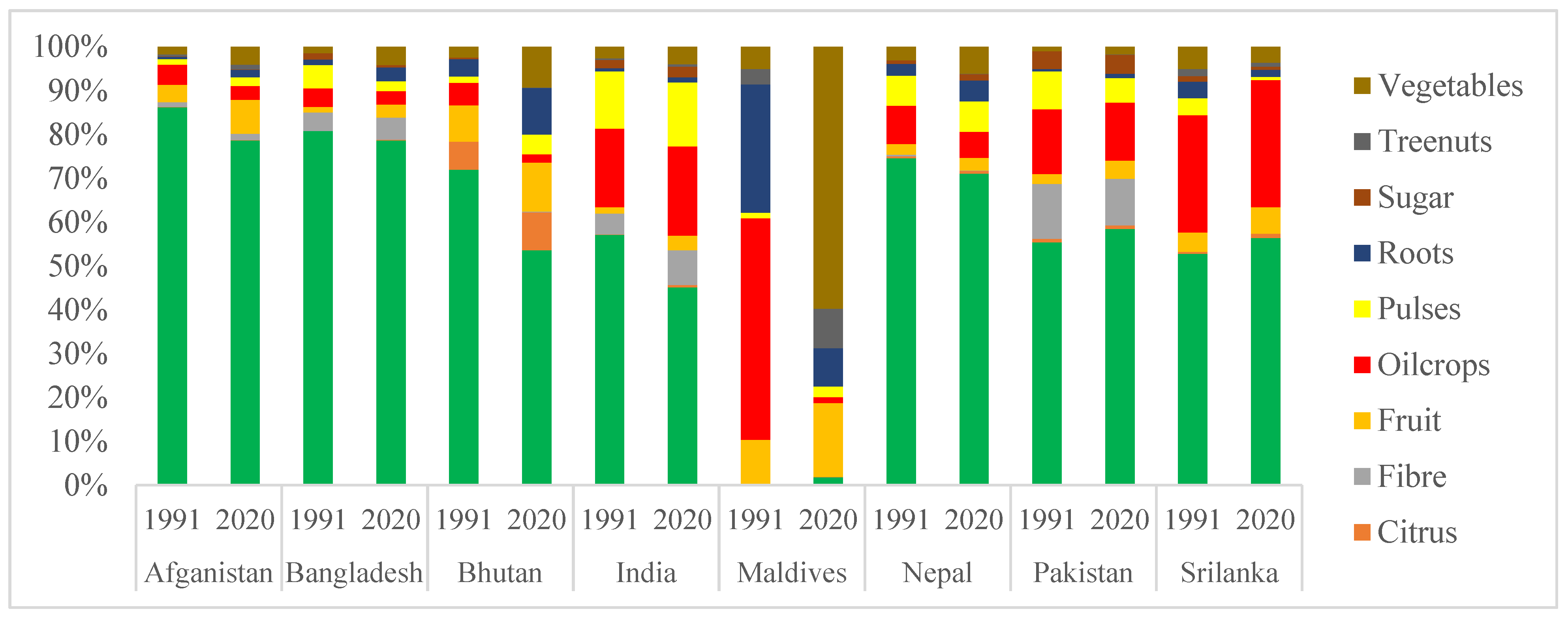
3.1. Cropping Pattern

Figure 1 depicts the share of cereals, citrus, fiber crops, fruit crops, oilseeds, pulses, root crops, sugar crops, tree nuts, and vegetables produced in Bangladesh, Bhutan, India, Pakistan, Nepal, Sri Lanka, Maldives, and Afghanistan from 1991 to 2020. Even though the share of cereals has decreased in most countries, cereals will continue to dominate South Asian agriculture in 2020. The area share under cereals ranges from 78 percent (Bangladesh) to 1.80 percent (Maldives). In India, the area under cereals decreased from 57.08 percent in 1991 to 45.13 percent in 2020, which was primarily replaced by fiber crops, fruits, oilseeds, pulses, and sugar crops, the share of these crops increased by 3.20, 1.92, 2.38, 1.57, and 0.48 percent, respectively, in 2020. Over the last three decades, there have been significant changes in the country’s oilseeds scenario, which is reflected in Figure 1 [20]. In 1991, oilseeds covered more than half of the agricultural land in the Maldives, but by 2020, the area under oilseeds was replaced by vegetables.

3.2. Dynamics of Cropping Pattern

Table 2. Change in area under different crops in different countries of South Asia (%).

Country		Cereals	Citrus	Fiber	Fruit	Oilseeds	Pulses	Roots	Sugar	Tree nuts	Vegetables
AFG	I	12.42	9.42	114.29	9.92	3.98	33.66	5.26	−31.25	−4.58	107.35
	II	32.67	−51.94	−34.00	47.80	−26.61	15.02	54.29	90.00	28.61	6.75
	III	−10.81	263.67	49.61	56.67	26.17	−6.40	178.37	−46.86	126.45	48.88
	IV	17.26	90.24	76.33	152.08	−12.26	100.55	329.07	−29.09	224.44	205.45
BGD	I	4.85	39.69	−26.82	11.20	−10.68	−25.39	69.67	−4.65	-	51.80
	II	2.04	129.04	−7.49	138.77	−8.31	−52.55	50.20	−23.02	-	56.09
	III	1.72	18.63	80.28	2.08	11.58	45.29	5.44	−30.44	-	37.03
	IV	10.43	337.97	34.61	178.75	−20.31	−51.77	191.42	−54.74	-	224.30
BTN	I	5.89	6.50	−10.31	10.31	−36.03	−15.32	8.06	0.24	-	35.81
	II	−10.41	−8.04	1.14	17.85	−50.37	19.72	32.22	4.87	-	73.01
	III	−46.18	−40.34	−18.27	−50.08	−39.61	38.50	5.07	−97.02	-	−19.76
	IV	−66.75	−39.88	−12.37	−39.52	−83.66	38.86	17.68	−96.83	-	68.99
IND	I	−0.43	76.98	14.24	47.72	9.50	−6.46	23.85	17.91	32.55	13.66
	II	−5.11	105.14	17.18	62.02	12.50	7.77	33.03	4.64	28.99	24.31
	III	−4.83	7.20	39.72	9.06	10.31	16.19	11.89	21.24	15.85	18.00
	IV	−7.11	399.07	96.54	174.64	33.04	31.65	82.71	47.17	98.93	78.75
MDV	I	-	-	-	−28.69	−21.74	15.38	−39.39	-	71.63	−28.24
	II	-	-	-	22.00	−62.50	11.70	−50.33	-	35.31	638.91
	III	-	-	-	48.55	−93.60	7.41	−17.99	-	−0.23	95.61
	IV	-	-	-	33.93	−97.87	48.72	−75.62	-	108.65	861.13
NPL	I	8.03	−11.33	−10.77	−12.60	16.67	2.74	23.21	71.09	34.03	14.41
	II	2.93	31.33	−25.29	40.32	−3.48	−0.57	48.69	−0.04	24.20	54.18
	III	1.21	24.06	−45.28	5.55	−32.93	15.66	5.29	17.42	68.20	20.72
	IV	12.79	60.33	−50.10	39.91	−19.95	20.74	103.40	127.38	204.17	138.91
PAK	I	5.49	14.08	11.89	32.94	15.40	−9.94	37.15	34.05	63.24	44.60
	II	7.94	0.67	6.02	35.77	8.04	1.89	28.41	1.56	−14.78	17.17
	III	4.28	1.55	−6.06	−9.12	−5.29	−14.85	36.39	10.39	−13.20	12.26
	IV	17.18	16.26	−5.30	101.23	−0.81	−28.46	131.99	20.29	18.27	95.04
LKA	I	4.23	27.43	-	44.05	4.98	−55.65	−36.43	−11.95	−18.46	−3.34
	II	15.19	42.92	-	2.32	−10.04	−22.79	−17.93	−23.42	−5.29	−0.02
	III	−9.20	0.71	-	−2.09	22.78	−40.68	−11.70	−12.73	−26.21	−14.28
	IV	17.41	107.66	-	53.27	19.19	−80.49	−53.44	−38.29	−35.55	−21.86

Note: Period I—1991–2000, Period II—2001–2010, Period III—2011–2020, and Period IV—1991–2020; AFG—Afghanistan, BGD—Bangladesh, BTN—Bhutan, IND—India, MDV—Maldives, NPL—Nepal, PAK—Pakistan, and LKA—Sri Lanka.

shows the percentage changes in the cropping pattern over three decades, namely Period I (1991–2000), Period II (2001–2010), Period III (2011–2020), and Period IV (1991–2020), representing the entire period for the eight South Asian countries. In 2020, the area under root crops increased by 329.07% over the base year of 1991 in Afghanistan, followed by tree nuts (224.44%), vegetables (205.45%), fruits (152.08%), and pulses (100.55%).

In contrast, the sugar crops and oilseeds cultivation decreased by 29.09 and 12.26 percent, respectively. Fiber (114.29%) and vegetables (107.35%) grew substantially in the period I while sugar crops increased by 90 percent in period II and citrus (178.37%) and tree nuts (126.45%) increased sharply in period III. Citrus, fruits, and vegetables reported remarkable growth in Bangladesh, with 337.97, 178.75, and 224.30 percent, respectively. In the period I, the area under roots (69.63%) and vegetables (51.80%) increased in Bangladesh. In contrast, in period II, the area under fruits (138.77%) and citrus (129.04%) increased by more than 50 percent, and in period III, the area under fiber crops increased by more than 80.28 percent. Except for vegetables, pulses, and roots crops, Bhutan’s area under all crops, including cereals, fruits, citrus, oilseeds, fiber, and sugar crops, has decreased over time. In Bhutan, vegetable area expanded rapidly in periods I and II, while sugar crops (97%) and fruits declined dramatically in period III (50%). Crop diversification toward high-value crops can enhance farm revenue, and the demand for high-value food items is expanding more rapidly than the demand for staple crops [21]. Table 2 also reveals that the area under cereals has decreased throughout all decades and the entire study period and has been primarily replaced by fruit and citrus cultivation in India. Except for cereals and pulses, all crops grew in period I, and all crops grew in period II and III, except cereals. A similar scenario was observed in the Maldives, where the area under oilseeds was replaced by vegetables and increased by 861.13%. In the Maldives, area under vegetables increased remarkably (638.90%) during Period II. The area under major cereals and oilseeds in Nepal has decreased over time, but it is expanding for high-value crops, such as vegetables (138.91%), tree nuts (204.17%), roots (103.40%), and fruits (39.91%) [22]. In period I, the area under all crops except citrus, fiber, and fruits; in period II, all crops except fiber, oilseeds, pulses, and sugar crops; in period III, the area under all crops increased except oilseeds. In Pakistan, the area under roots, fruit, and vegetables increased by 131.99, 101.23, and 95.04 percent over the entire period. The area under all the crops increased except pulses in period I, tree nuts in period II, and remarkable growth was recorded by the cereals, citrus, root crops, sugar crops, and vegetables in period III. In Sri Lanka the area under pulses, root crops, sugar crops, tree nuts, and vegetables declined substantially in all the periods under study.

3.3. Growth of Cropping Pattern

The compound annual growth rate (CAGR) in the cropping pattern over three decades, namely Period I (1991–2000), Period II (2001–2010), Period III (2011–2020), and Period IV (1991–2020) is shown in

Table 3. Growth rates of area under crops in different countries of South Asia pattern.

Country		Cereals	Citrus	Fiber	Fruits	Oilseeds	Pulses	Roots	Sugar	Tree Nuts	Vegetables
AFG	I	1.9 **	0.8	4.2	1.2 ***	−0.7	4.6 **	0.6 ***	−2.0	−0.2	4.5 **
	II	3.6 ***	−10.5 ***	−4.6 *	4.5 ***	3.5 ***	0.8	5.0 ***	12.3 ***	4.2 ***	1.2
	III	3.4 **	13.8 ***	3.6 **	7.5 ***	5.2 **	2.0	9.6 ***	−12.1 ***	7.9 ***	4.9 **
	IV	0.4	1.3 *	1.6 ***	3.3 ***	3.0 ***	2.7 ***	3.7 ***	1.0	3.6 ***	1.2 ***
BGD	I	0.4	4.7 ***	−2.5 **	1.3 ***	−0.6 *	2.2 ***	3.0 *	−0.8 ***	-	3.1 ***
	II	0.1	9.7 ***	0.7	12.1 ***	−1.2 ***	−9.0 ***	5.7 ***	−2.6 ***	-	6.3 ***
	III	0.2	2.1 *	3.6 **	−0.8	2.3 ***	4.7 ***	0.9**	−3.7 ***	-	3.6 ***
	IV	0.5 ***	5.9 ***	1.1 **	4.3 ***	−0.8 ***	−3.7 ***	4.7 ***	−2.6 ***	-	4.3 ***
BTN	I	1.4 **	−2.6	−0.4	−1.0	−4.9 ***	−0.4	−1.5	0.001	-	−0.5
	II	0.6	−1.3	1.0	3.6 *	−3.0	3.6 *	4.3 ***	0.5 ***	-	8.7 ***
	III	−6.1 ***	−8.4 ***	−0.7	−10.9 ***	−3.9	2.2 **	−0.8	−56.4 ***	-	−5.1 *
	IV	−3.3 ***	−1.1 **	−0.2	−0.9	−6.5 ***	1.5 ***	−0.8 ***	−11.7 ***	-	1.8 ***
IND	I	0.02	8.3 ***	2.3 ***	3.9 ***	1.1 ***	−0.7 **	2.0 ***	1.8 **	3.4 ***	1.8 **
	II	−0.02	9.2 ***	1.7 **	6.0 ***	2.3 ***	1.8 **	4.0 ***	1.2	2.8 ***	2.0 **
	III	−0.04 **	2.2 *	1.7	0.7	0.2	2.8 ***	1.5 ***	0.5	1.1 **	1.7 ***
	IV	−0.08 **	6.2 ***	1.7 ***	3.6 ***	7.0 ***	1.2 ***	2.3 ***	1.2 ***	2.5 ***	2.5 ***
MDV	I	31.8 ***	-	-	−2.3	−1.1	2.3 ***	−5.2 ***	-	7.7 ***	−3.0 ***
	II	−0.6	-	-	6.9 **	−27.8 ***	2.3	−9.2 ***	-	4.9 ***	13.9 *
	III	2.3 ***	-	-	3.9	29.7 ***	0.6 **	−2.5 ***	-	0.1	11.2 ***
	IV	8.5 ***	-	-	−1.2 *	−14.7 ***	1.7 ***	−5.4 ***	-	2.6 ***	9.9 ***
NPL	I	1.3 ***	−3.6 *	−1.2	−3.3 **	1.9 ***	0.4	2.5 ***	5.6 ***	3.2 ***	1.7 **
	II	0.4 ***	1.9	−1.8 *	3.2 ***	−0.2	0.3	3.5 ***	0.5	2.3 ***	4.8 ***
	III	−0.02	2.0 ***	−6.3 ***	0.3	−4.9 **	1.7 ***	0.7 **	2.5 ***	3.8 ***	2.0 ***
	IV	0.5 ***	2.1 ***	−2.0 ***	2.8 ***	−0.08	0.4 ***	3.0 ***	2.6 ***	3.8 ***	3.3 ***
PAK	I	0.8 ***	1.6 ***	1.1 **	3.4 ***	1.6 ***	−0.7 *	3.7 ***	2.7 ***	4.0 ***	4.1 ***
	II	1.2 ***	0.5	0.2	4.1 ***	0.9 *	0.7 **	3.6 ***	0.8	−1.5 ***	2.6 ***
	III	0.7 **	0.4 **	−1.5 *	−0.9 ***	1.7 **	1.8 ***	2.4 ***	1.8	−1.6 ***	1.3 ***
	IV	0.6 ***	0.3 ***	−0.3 *	2.9 ***	−0.2	−1.1 ***	3.3 ***	0.8 ***	−0.5 **	2.1 ***
LKA	I	−0.6	2.6 ***	-	4.3 ***	0.7 ***	−10.8 ***	−4.4 ***	−1.4	−2.7 ***	−0.4
	II	2.4 *	4.0 ***	-	0.1	−1.5 ***	−2.4 *	−2.2 ***	−3.3 ***	−1.0 *	0.9
	III	−1.4	−0.4	-	−0.4	2.2 ***	−4.6 ***	−1.6 ***	1.5	−3.5 ***	−1.9 **
	IV	1.3 ***	2.9 ***	-	1.3 ***	0.2	−5.4 ***	−2.1 ***	−1.4 ***	−0.7 ***	−0.5 ***

Note: ***, ** and * indicates significant at 0.01, 0.05 and 0.10 level; Note: Period I—1991–2000, Period II—2001–2010, Period III—2011–2020 and Period IV—1991–2020; AFG—Afghanistan, BGD—Bangladesh, BTN—Bhutan, IND—India, MDV—Maldives, NPL—Nepal, PAK—Pakistan, and LKA—Sri Lanka.

. The area under citrus, fiber, fruits, oilseeds, pulses, roots, roots, and vegetables increased significantly in Afghanistan over the entire period (1991–2020), with annual growth rates of 1.3, 1.6, 3.3, 3, 2.7, 3.7, 3.6, and 1.2 percent, respectively. The cultivation of cereals, citrus, fiber, fruits, roots, and vegetables increased significantly in Bangladesh from 1991 to 2020, while cultivation of oilseeds, pulses, and sugar crops decreased significantly.

The CAGR of all crops in Bhutan was negative, except for pulse crops, which increased by 1.5% per year. In India, the area under cereals has been replaced by high-value crops, and it can be seen from Table 3 that, aside from cereals, the area under high-value crops has increased significantly. The vegetable and cereal area has increased by 9.9 and 8.5 percent, respectively, while the area under oilseed crops has decreased by 14.7% per year in the Maldives. In Nepal, the annual growth rates for cereals, citrus, fruits, pulses, roots, and vegetables were 0.5, 2.1, 2.8, 0.4, 3.0, and 3.3 percent, respectively. The cultivation of cereals, citrus fruits, roots, sugar crops, and vegetables increased significantly in Pakistan, but only cereals, citrus fruits, and oilseeds increased significantly in Sri Lanka.

3.4. Panel Data Unit Root Testing

Before analyzing the determinants of crop diversification, it is necessary to determine whether the determinants are free of unit roots. We use the Levin–Lin–Chu and Im–Pesaran–Shin root tests to assess stationarity in a 30-year panel data set [23]. The majority of the determinants (arable land ha/person, cropland percent, population, merchandise index, temperature (maximum and minimum), rainfall, food crop yield index, and non-food crop yield index), according to the Levin–Lin–Chu test, were stationary at the level, while the rest became the stationary first difference. The Im–Pesaran–Shin test gives similar results in cropland percent (share), merchandise index, temperature (maximum and minimum), root zone moisture, rainfall, fertilizer, pesticide, food crop yield index, and non-food crop yield index were stationary at a level. At the same time, other determinants, such as arable land ha/person, per capita gross domestic product, and the population became the stationary first difference (

Table 4. Stationarity testing.

Particulars	Levin–Lin–Chu Test	Im–Pesaran–Shin Test
Entropy diversification Index	First difference **	At level *
Arable land ha/person	At level **	First difference **
Per capita G.D.P. (USD)	First difference **	First difference **
Cropland percent (share)	At level **	At level **
Population (’000 person)	At level **	Second difference **
Merchandize index	At level **	At level **
Temperature (maximum)	At level **	At level **
Temperature (minimum)	At level **	At level **
Root zone moisture	First difference **	At level **
Rainfall (mm)	At level *	At level **
Fertilizer (kg/ha)	Second difference **	At level *
Pesticide (kg/ha)	Second difference *	First difference **
Food crop yield index	At level *	At level **
Non-food crop yield index	At level *	At level **

Note: ** and * indicates significant at 0.01 and 0.05 level.

).

3.5. Model Specification

In a regression model, the Hausman specification test finds endogenous repressors (predictor variables) [24]. It is also called a model misspecification test. In panel data analysis, the Hausman test permits the selection of a fixed-effects model (FEM) or a random-effects model (REM), and the findings are provided in

Table 5. Hausman model specification test.

Hypothesis	Hausman Test	Test Statistics	p-Value	Model Selection
Ho = FEM H1 = REM	χ2	7.16	0.519	Random effect model

. On the basis of test parameters, a random effect model was selected.

3.6. Determinants of Crop Diversification

The results of the random effect model using panel data regression are shown in Table 5. The estimated R-square was 0.69, implying that all of the determinants listed in

Table 6. Estimates of random effect model.

Particulars	Model- Entropy Diversification Index
	Coefficient
Arable Land ha/person	−0.054 (0.108)
G.D.P. per capita USD	0.00005 *** (~0)
Crop land per cent (Share)	−0.049 *** (0.009)
Population (’000 person)	−0.000004 *** (~0)
Merchandise index	−0.039 (0.074)
Temperature (Maximum)	0.0006 (0.002)
Temperature (Minimum)	0.003 *** (0.001)
Root zone moisture	−0.055 (0.055)
Rainfall (mm)	0.000002 (~0)
Fertilizer (kg/ha)	0.00003 (~0)
Pesticide (kg/ha)	0.0005 *** (0.0001)
Food crop yield index	0.0004 *** (0.0001)
Non-food crop yield index	0.0005 ** (0.0003)
Countries
Bangladesh	0.759 *** (0.162)
Bhutan	0.017 (0.033)
India	0.985 *** (0.116)
Maldives	0.313 *** (0.074)
Nepal	0.144 *** (0.029)
Pakistan	0.732 *** (0.084)
Sri Lanka	0.441 *** (0.075)
Intercept	0.472 *** (0.100)
σe	0.0369
Overall R2	0.69

Note: Indicates *** and ** significant at 0.01 and 0.05 level; figure in parenthesis are robust standard error of the respective coefficient.

together explained 69 percent of the total variations in the crop diversification index. The results showed that per capita gross domestic product (USD), temperature (minimum), pesticide use, food crop yield index, and non-food crop yield index have a statistically positive and significant impact on crop diversification in South Asian agriculture throughout the study period [25]. Similar results also presented agricultural gross capital formation and services sector GDP., which contribute significantly to agricultural productivity growth in Pakistan and India [26]. In addition, merchandize index revealed negative relation with crop diversification and similar results were found in sources of agricultural productivity growth in South Asian Association for Regional Cooperation (SAARC) countries, indicating that trade negatively impacts agricultural growth in the short run [27].

On the other hand, cropland percent (share) and population have a significant negative impact on crop diversification. The maximum temperature, rainfall, and fertilizer on the entropy diversification index was positive but not statistically significant. Increases in all determinants have a significant and positive impact in Bangladesh, India, Maldives, Nepal, Pakistan, and Sri Lanka, leading to crop diversification within these countries, but have a significant negative impact in Bhutan, where crop diversification increases but not significantly. The current status of crop diversification and its various determinants are presented in Figure 2. The figure also shows that Afghanistan and Bangladesh have the most diverse agriculture, followed by Nepal, Pakistan, Bhutan, and Indian agriculture being more specialized. Afghanistan, the most diverse country, has the highest fertilizer consumption and rainfall, which do not affect diversification. The area under food crops significantly impacts crop diversification, as evidenced by the extent of crop diversification and the food crop yield index in Afghanistan (Table 5 and Figure 2). Bangladesh and Sri Lanka use the most pesticides, followed by Pakistan and India, with Nepal and Bhutan using the least.

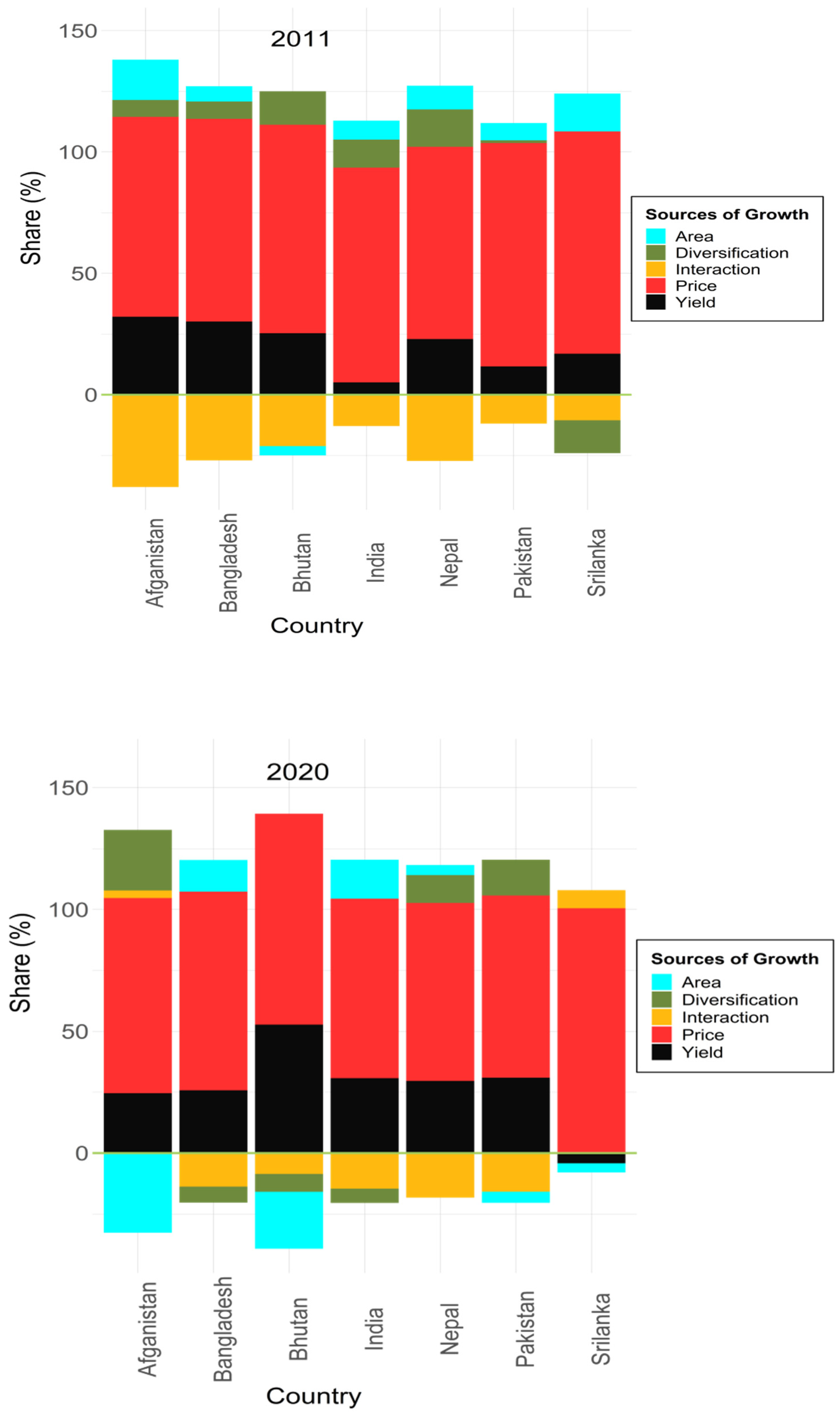
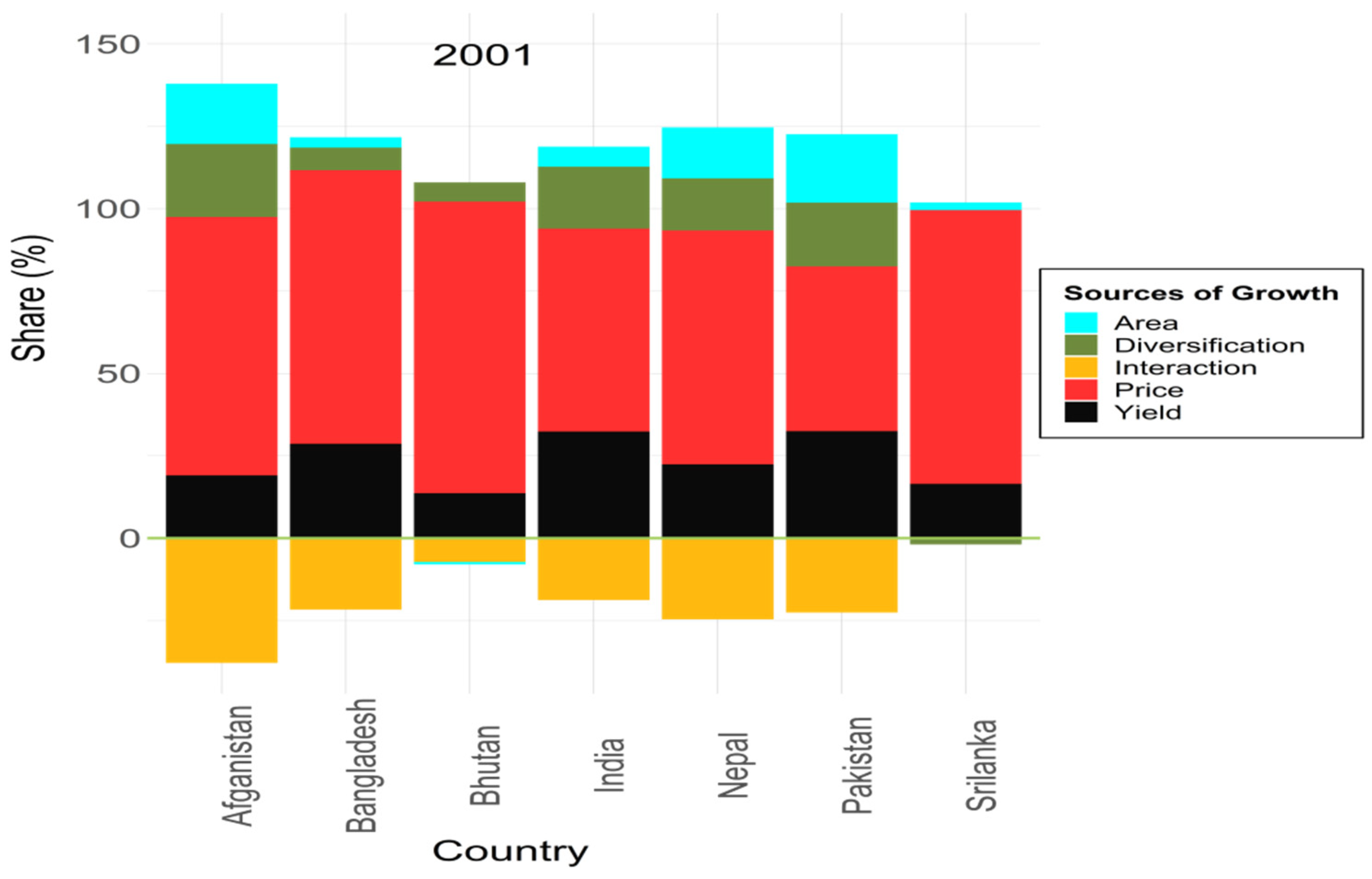
3.7. Sources of Agriculture Growth

Table 7. Share of various sources to income growth during 2001–2020 (%).

Country	Year	Area	Yield	Price	Diversification	Interaction
Afghanistan	2001	18.29	19.04	78.44	22.13	−37.91
	2011	16.61	32.10	82.37	6.96	−38.04
	2020	−32.72	24.60	80.14	24.88	3.11
Bangladesh	2001	3.16	28.64	83.01	6.87	−21.68
	2011	6.29	30.14	83.52	7.14	−27.09
	2020	13.00	25.76	81.59	−6.59	−13.76
Bhutan	2001	−0.72	13.63	88.51	5.84	−7.25
	2011	−3.82	25.32	85.89	13.79	−21.18
	2020	−23.39	52.75	86.54	−7.35	−8.55
India	2001	6.08	32.36	61.58	18.78	−18.80
	2011	7.82	5.07	88.46	11.56	−12.92
	2020	15.99	30.76	73.72	−5.88	−14.59
Nepal	2001	15.47	22.37	71.00	15.81	−24.65
	2011	9.75	22.93	79.21	15.41	−27.31
	2020	4.12	29.63	73.06	11.48	−18.30
Pakistan	2001	20.80	32.45	50.01	19.34	−22.59
	2011	7.09	11.66	92.01	1.16	−11.93
	2020	−4.59	30.93	74.85	14.67	−15.87
Sri Lanka	2001	2.33	16.46	83.11	−1.67	−0.23
	2011	15.63	16.90	91.55	−13.52	−10.55
	2020	−3.76	−4.18	100.56	−0.02	7.41

shows the decomposition of agricultural growth into area effect, yield effect, price effect, and diversification over three time periods: 2001, 2011, and 2020 as visualized in Figure 3. A clear understanding of the drivers of agricultural growth is essential to assess the current trends in sustainability and identify future policy priorities.

Output prices contributed more than half of agricultural growth and remained the primary source of growth in all South Asian countries. The yield was identified as the second important factor. In 2020, agricultural crop yields contributed 24.60, 25.76, 52.75, 30.76, 29.63, and 30.93% in Afghanistan, Bangladesh, Bhutan, India, Nepal, and Pakistan, respectively. The contribution of crop diversification to agricultural growth has decreased over time, but in Afghanistan, Nepal, and Pakistan, it contributed 24.88 percent, 11.48 percent, and 14.67 percent, respectively, in 2020. The decomposition of agricultural growth into area effect, yield effect, price effect, and diversification is presented in Figure 3. The price effect has been positive in all the South Asian countries, contributing from 50 percent (2001) to 100.56 percent (2020) among the different countries. Moreover, the price effect showed an increasing trend with time in all the countries; in the current period, Sri Lanka has shown the highest (100.56%) and Nepal the lowest (73.06). During the study period, the yield effect was positive in all the countries except Sri Lanka. India, Pakistan, and Afghanistan have shown similar yield effects during the study period, which ranges from 30 percent to 33 percent in all decades. However, Sri Lanka negatively affected the yield, which decreased the agriculture growth by 4 percent in the decade 2011 to 2020 [25,28]. Agricultural growth has been influenced by crop diversification in all the South Asian countries from 1991 to 2010, except Sri Lanka has had a negative impact on agricultural transformation. From 2011 to 2020, crop diversification negatively affected agricultural growth in Sri Lanka, India, and Bangladesh. In addition, crop diversification has considerably affected Afghanistan’s agriculture growth, which impacts more than 20 percent in all decades [25,29]. Sri Lanka Agricultural sector revealed that sources of growth, such as area, crop diversification, and yield effects, are negative, then the sources of agriculture growth were price effect. Agricultural growth was influenced by India’s area, yield, and price effects. However, crop diversification positively affected the agriculture growth from 1991 to 2010 but was still decreasing and negative during the last decade. Indian government should give an intention towards increasing crop diversification, which was the primary source of agricultural transformation in the future. We have also discussed in the introduction that some South Asian countries are deficient in food grain production. The study concluded that crop diversification is essential for achieving higher output growth, increasing farm income, creating jobs, conserving precious soil and water resources, consumer preferences for high-value, nutrient-dense foods, rural livelihood, sustainable use of natural resources, and poverty alleviation. Thus, in South Asia, Sri Lanka and Bhutan have lost most of their crop area for the studied commodities and can be termed as the least diversified countries.

Figure 2. Status of crop diversification and their determinants in different countries of South Asia (generated through ArcGIS 10.2.2, from a public domain shape file using World Bank Official Boundaries [30]. Note: Political boundary of countries may differ).

Figure 2. Status of crop diversification and their determinants in different countries of South Asia (generated through ArcGIS 10.2.2, from a public domain shape file using World Bank Official Boundaries [30]. Note: Political boundary of countries may differ).

Figure 3. Sources of agricultural growth in different countries of South Asia (2001, 2011, and 2020).

Figure 3. Sources of agricultural growth in different countries of South Asia (2001, 2011, and 2020).

4. Conclusions

This study investigated crop diversification status and determinants in eight South Asian countries, considering socioeconomic, soil/agronomic, agricultural inputs, the productivity of food and non-food crops, international trade, and climate factors. All these determinants considered explained 69 percent of the total variations in the crop diversification index. The crop diversification in South Asia was influenced by per capita GDP, minimum temperature, pesticide consumption, food crop yield index, and non-food crop yield index during the study period. The percentage of cropland and population, on the other hand, negatively influence crop diversification. All the determinants in the study have shown significant and positive impact for Bangladesh, India, the Maldives, Nepal, Pakistan, and Sri Lanka, leading to crop diversification while negatively impacting crop diversification in Bhutan. Afghanistan and Bangladesh have more diverse agriculture in the study area, followed by Nepal, Pakistan, Bhutan, and India. The most diverse country, Afghanistan, has the highest fertilizer consumption and rainfall, neither of which affects diversification. In 2020, the output price contributed to more than half of agricultural growth. It remains the primary source of growth in all South Asian countries, with yield being identified as the second most important factor. The contribution of crop diversification to agricultural growth has been declining over time. Except for Afghanistan, Pakistan, and Nepal, no other country has achieved agricultural growth with a contribution from diversification. This growth is not sustainable in the long run as yield is stagnating and area suitable for crop cultivation is limited. This can be used as a warning sign by the countries to frame appropriate agriculture policies for making agriculture more diversified in the coming decades for sustaining food and nutritional security.

References

1. Birthal, P.S.; Joshi, P.K.; Roy, D.; Pandey, G. Transformation and Sources of Growth in Southeast Asian Agriculture; IFPRI Discussion Paper 1834; International Food Policy Research Institute (IFPRI): Washington, DC, USA, 2019. [Google Scholar]
2. Food and Agriculture Organization. FAO STAT. 2022. Available online: http://www.fao.org/faostat/en/#data (accessed on 5 May 2022).
3. Food and Agriculture Organization. The Future of Food and Agriculture–Trends and Challenges; F.A.O.: Rome, Italy, 2017; pp. 1–180. [Google Scholar]
4. Kaur, M.; Guleria, A.; Singh, J.; Kingra, H.S.; Singh, S. Emerging Policy Concerns for Improving Input Use Efficiency in Agriculture for Global Food Security in South Asia. In Input Use Efficiency for Food and Environmental Security; Bhatt, R., Meena, R.S., Hossain, A., Eds.; Springer: Singapore, 2021; pp. 687–705. [Google Scholar] [CrossRef]
5. Joshi, P.K.; Birth, P.S.; Minot, N. Sources of Agricultural Growth in India: Role of Diversification Toward High-Value Crops; MTID Discussion Paper No. 85; International Food Policy Research Institute: Washington, DC, USA, 2006. [Google Scholar]
6. Von Braun, J. Agricultural commercialization: Impact on income and nutrition and implications for policy. Food Policy 1995, 20, 187–202. [Google Scholar] [CrossRef]
7. Pingali, P.L.; Rosegrant, M.W. Agricultural commercialization and diversification: Processes and policies. Food Policy 1995, 20, 171–186. [Google Scholar] [CrossRef]
8. Chand, R. Diversification through high value crops in western Himalayan region: Evidence from Himachal Pradesh. Indian J. Agric. Econ. 1996, 41, 652–663. [Google Scholar]
9. Ryan, J.G.; Spencer, D.C. Future Challenges and Opportunities for Agricultural R&D in the Semi-Arid Tropics; International Crops Research Institute for the semi-Arid Tropics: Andhra Pradesh, India, 2001. [Google Scholar]
10. Birthal, P.S.; Joshi, P.K.; Gulati, A. Vertical Coordination in High Value Commodities: Implications for Smallholders; MTID Discussion Paper No. 85; International Food Policy Research Institute: Washington, DC, USA, 2005. [Google Scholar]
11. Kumar, S.; Gupta, S. Crop Diversification towards High-value Crops in India: A State-Level Empirical Analysis. Agric. Econ. Res. Rev. 2015, 28, 339–350. [Google Scholar] [CrossRef]
12. Kumar, S.; Kumar, S.; Chahal, V.P.; Singh, D.R. Trends and determinants of crop diversification in Uttar Pradesh. Indian J. Agric. Sci. 2018, 88, 1704–1708. [Google Scholar]
13. N.U.N. Comtrade Database. 2022, International Trade Statistics Database. Available online: https://comtrade.un.org (accessed on 5 May 2022).
14. NASA. Power Data Access Viewer. 2022. Available online: https://power.larc.nasa.gov/data-access-viewer (accessed on 16 May 2022).
15. Singh, P.; Guleria, A.; Vaidya, M.K.; Sharma, S. Determinants of diversification in relation to farm size and other socioeconomic characteristics for sustainable hill farming in Himachal Pradesh. Indian J. Econ. Dev. 2020, 16, 418–424. [Google Scholar]
16. Singh, P. An Economic Analysis of Vulnerability and Impact of Climate Change on Agriculture in Himachal Pradesh. Ph.D. Thesis, Dr. YS Parmar University of Horticulture and Forestry, Nauni, India, 2021. [Google Scholar]
17. Minot, N.; Epprecht, T.T.M.; Tram, A.; Trung, L.Q. Income Diversification and Poverty in Northern Uplands of Vietnam; Research Report. 145; International Food Policy Research Institute: Washington, DC, USA, 2006. [Google Scholar]
18. Joshi, P.K.; Gulati, A.; Birth, P.S.; Tewari, L. Agriculture Diversification in South Asia: Patterns, Determinants, and Policy Implications; MSSD Discussion Paper No. 57. International Food Policy Research Institute: Washington, DC, USA, 2003; Available online: http://www.cgiar.org/ifpri/divs/mssd/dp.htm (accessed on 4 May 2022).
19. Pandey, G.; Kumari, S. Understanding agricultural growth and performance in Bihar, India. SN Bus. Econ. 2021, 1, 145. [Google Scholar] [CrossRef]
20. Kumar, T. Sparking Yellow Revolution in India Again. 2020. Rural Pulse. JUNE JULY 2020 ISSUE XXXIV. Available online: https://www.nabard.org/auth/writereaddata/tender/2106212557Rural%20Pulse%20Issue%20XXXIV%20 (accessed on 25 April 2022).
21. Birthal, P.S.; Joshi, P.K.; Roy, D.; Thorat, A. Diversification in Indian Agriculture Toward High-Value Crops: The Role of Small Farmers. Can. J. Agric. Econ. 2013, 61, 61–91. [Google Scholar] [CrossRef]
22. Thapa, G.; Kumar, A.; Joshi, P.K. Agricultural Diversification in Nepal: Status, Determinants, and Its Impact on Rural Poverty; IFPRI Discussion Paper 1634; International Food Policy Research Institute (IFPRI): Washington, DC, USA, 2017; Available online: http://ebrary.ifpri.org/cdm/ref/collection/p15738coll2/id/131153 (accessed on 25 April 2022).
23. Jaroslava, H.; Wagner, M. The Performance of Panel Unit Root and Stationarity Tests: Results from a Large Scale Simulation Study. Econom. Rev. 2006, 25, 85–116. [Google Scholar] [CrossRef] [Green Version]
24. Hausman, J.A. Specification tests in econometrics. Econom. J. Econom. Soc. 1978, 1, 1251–1271. [Google Scholar] [CrossRef] [Green Version]
25. Morita. Chapter 7—Past growth in agricultural productivity in South Asia. Curr. Dir. Water Scarcity Res. 2021, 3, 137–156. [Google Scholar]
26. Zulfiqar, B.; Munir, A. The Role of Agricultural Growth in South Asian Countries and the Affordability of Food: An Inter-country Analysis. Pak. Dev. Rev. 2000, 39, 751–767. Available online: https://www.jstor.org/stable/41260296 (accessed on 25 April 2022).
27. Ali, N.; Hayat, U.; Ali, S.; Khan, M.I.; Khattak, S.W. Sources of agricultural productivity growth in SAARC countries: The role of financial development, trade openness and human capital. Sarhad J. Agric. 2021, 37, 586–593. [Google Scholar] [CrossRef]
28. Liu, J.; Wang, M.; Yang, L.; Rahman, S.; Sriboonchitta, S. Agricultural productivity growth and its determinants in south and southeast asian countries. Sustainability 2020, 12, 4981. [Google Scholar] [CrossRef]
29. Rosegrant, M.W.; Evenson, R.E. Agricultural Productivity and Sources of Growth in South Asia. Am. J. Agric. Econ. 1992, 74, 757–761. [Google Scholar] [CrossRef]
30. World Bank Official Boundaries. Available online: https://datacatalog.worldbank.org/search/dataset/0038272 (accessed on 16 May 2022).
Figure 1. Share of different crops in the total cultivated area of different countries of South Asia (%).
Sustainability 14 09363 g001