Prediction of China’s Economic Structural Changes under Carbon Emission Constraints: Based on the Linear Programming Input–Output (LP-IO) Model

Abstract

China has established a carbon emission reduction goal for 2030. For the Chinese government, there is a dilemma between reducing carbon emissions while still striving to maintain continuous economic growth in future. To achieve these “dual goals”, it is necessary to predict the optimal industrial structure under these constraints in 2030. By integrating the linear programming input–output model (LP-IO) with the RAS updating technique, this paper predicts the industrial structure in China in 2030 and compares it with the year 2018. The results show that China’s industry structure will experience major changes. In particular, most of the industries related to manufacturing, such as mining, petroleum, and metal, will lose their important positions in the economic system, while service industries such as culture, sports, and public service will take over the position as pillars of the economy. Additionally, carbon emissions in 2030 will be at least 12.8 billion tons. Based on these findings, it is suggested that the Chinese government should increase investment in service industries in advance to meet the goal of reducing carbon emissions earlier.

1. Introduction

Currently, China is the country with the largest amount of carbon emissions in the world [1]. In recent years, China has been committed to reducing carbon emissions and taking responsibility for protecting the global environment. The measures it has taken include setting carbon emissions targets, building a carbon emission trading market, reducing energy consumption, updating industrial production technologies, enriching renewable energy, developing carbon capture projects, and so on. In 2020, the Chinese government officially announced the “3060” goals of “carbon emission reduction” and “carbon neutrality”, that is, to achieve carbon peaking by 2030 and achieve carbon neutrality by 2060 [2]. At the same time, as the largest developing country in the world, China still faces developmental challenges, and the Chinese government will also strive to maintain stable economic growth in the future. Over the past decades, China has been one of the fastest-growing countries in the world, lifting hundreds of millions of people out of poverty. The absolute poverty rate of China fell from 66.3% in 1990 to 0.1% in 2019, and this has made an outstanding contribution to solving the global hunger problem [3]. China’s industrialization development has also been helpful to the prosperity of the global industrial chain and provided support for reducing global commodity costs. Therefore, from the perspective of the Chinese government, achieving steady economic growth is still the bottom line. The Chinese government has set economic goals every year. For example, at the beginning of 2022, the Chinese government announced a minimum expected GDP growth target of 5.5% in 2022 [4,5], and it is very likely that China will set an annual GDP growth target of 3–5% in the next few years.

The Chinese government has realized the importance and urgency of reducing carbon emissions, and measures were being implemented from years ago. However, China’s carbon emissions have continued to grow without a significant decline trend [6]. As we approach 2030, the Chinese government is under increasing pressure. Additionally, China’s carbon emissions mainly come from energy, manufacturing industries, and construction [6]. Therefore, to achieve the “dual goals”, China must adjust its economic and industrial structure to focus on the development of and investment in industries with low carbon emissions and to restrict investment into industries with high carbon emissions.

To predict what changes will occur to China’s economic structure by 2030 under the “dual goals” aim, this paper incorporates the dual goals into the linear programming input–output model and obtains the optimal output for every industry in 2030. Then, by using the input–output table update technology, the consumption matrix of China in 2030 is predicted. Comparing the predicted input–output matrix in 2030 with that from 2018, this paper analyzes the trend of change in China’s industries during these years under such conditions.

The remainder of this paper is as follows: Section 2 is a literature review which mainly reviews the related literature in which other scholars used the input–output model for industry analysis or for carbon emission prediction and summarizes the advantages and disadvantages of this literature. Section 3 is the methodology that is applied in this paper, which illustrates the LP-IO model and RAS update technique. Section 4 elaborates on data sources and conducts empirical an analysis based on the models in Section 3. Section 5 discusses the analytical results and provides recommendations. Section 6 includes the conclusion.

2. Literature Review

An input–output model is an analytical method to study the rule of value flow, internal correlation, quantity dependence, and supply–demand balance between various sectors of the national economy. The idea of input–output was originally proposed and expanded by Professor Wassily Leontief, who won the Nobel Prize in Economics in 1973 [7,8]. Since the input–output model was proposed, it has not only been rapidly applied in the analysis of national economic system and its industries, but also widely used in supply chain value analysis, disaster impact, environmental protection, and other areas [9,10]. Allan et al. [11] extended the input–output model to introduce the pollution sector and wastewater treatment sector to analyze the impact on society and the environment. Andrew et al. [12] studied carbon transfer between countries through the multiple region input–output table (MRIO) and found that the emissions reflected in imports between countries accounted for 40% of the total emissions on average. Li et al. [13] built a disaster prediction method through an input–output model in London City, and the results showed that it would take about 70 months to recover after assuming that London would be hit by a flood. After combing with other models, the application field of the input–output model is greatly expanded. For example, Igos et al. [14] combined the input–output model, the CGE model (computable general equilibrium) to assess the environmental impact of different energy policies in Luxembourg from 2010 to 2025. Liu et al. [15] combined the grey neural network model with the input–output model to predict energy consumption under different economic growth scenarios.

Linear programming input–output model (LP-IO) combines input–output and linear programming model, which was initially mainly used to analyze optimization problems in macroeconomics [16,17], especially in economic strategy planning [18]. At present, the LP-IO model is gradually starting to be used for environmental protection issues. San Cristóbal [19] took Spain as the research object and used the LP-IO model to analyze the impact of setting greenhouse gas emission reduction targets on production activities. Lin [20] applied the LP-IO model to evaluate the changes in wastewater treatment industry under the conditions of minimizing land use, carbon emissions, and temperature changes by using the Tokyo Metropolitan Input–Output Table. Danielle et al. [21] built the LP-IO model and took the Philippines as the research object to measure the fluctuation of economic growth in the event of a collapse of the energy system. Nguyen et al. [22] used the LP-IO model to study Vietnam’s carbon emission goals in 2030 and found that with management measures, Vietnam’s greenhouse gas emissions in 2030 will be reduced by 24.6%.

As China is currently the country with the largest carbon emissions, many studies use the optimal input–output model to analyze China’s carbon emissions. Kang et al. [23] used the LP-IO model to study China’s carbon emission trends, and the results show that from 2020 to 2050, if no emission restriction targets are set, China’s cumulative CO₂ emissions will increase by 30% from the normal level. Su et al. [24] used the optimal model to analyze the goal of China emission in 2030, and it shows that China can peak its CO₂ emissions by 2030 with the optimized industrial structure. Yu et al. [25] studied the time for China to reach its carbon peak and showed that the Chinese government must adjust China’s industrial structure to achieve the goal as expected.

In summary, these literatures use the LP-IO model to study environmental issues and China’s carbon emissions, but most of them focus on when the total carbon emissions will peak. Few studies focus on the expected adjustment of China’s economic structure under the constraints of carbon emissions and rarely analyze industry change by using input–output table updating techniques. Under the dual goals, restricting the development of some industries will inevitably affect all industries in China. Considering that the economy is an interactive system in which industries support and supply each other, it is necessary to deepen analyses and reasonably predict the potential changes within different industries. This paper applies a LP-IO model and RAS technique to predict the input–output table of 2030 under dual goals and then analyzes the influence effect and sensitivity effect both in 2018 and 2030, which provides a new perspective for estimating industrial change. Additionally, because the databases used in this study are usually updated yearly, it is convenient to set up an auto-updated prediction approach by using IA techniques.

3. Methodology

3.1. Input–Output Model and I-O Table

3.1.1. Basic Framework

The input–output model can illustrate the circular economy activities of production and reproduction, which are mainly described by the input–output table. The input–output table arranges the initial input and intermediate input vertically and sets the intermediate use and final use horizontally. The basic input–output table is shown in

Table 1. Basic input–output table.

		Intermediate Demand				Final Demand	Total Output
		1	2	…	n
Intermediate Input	1	$x_{11}$	$x_{12}$	…	$x_{1n}$	$y={\displaystyle {\displaystyle \sum }_{i=1}^n}{y}_i$	$x_{out}={{\displaystyle \sum }}_{i=1}^n{x}_i$
	2	$x_{21}$	$x_{22}$	…	$x_{2n}$
	…	…	…	…	…
	n	$x_{n1}$	$x_{n2}$	…	$x_{nn}$
Initial Input (GDP)		$n={\displaystyle {\displaystyle \sum }_{j=1}^n}{n}_j$
Total Input		$x_{in}={\displaystyle {\displaystyle \sum }_{j=1}^n}{x}_j$

below.

Within the table: $x_{ij}$ is an element in the table; from the horizontal view, it represents the quantity of product $i$ allocated to department $j$. From the vertical column, it represents the quantity of product $i$ consumed in the production of department $j$. $x_{ij}$ is the key element connecting input and output relations between different sectors. $n$ is the initial input, which includes items such as the depreciation of fixed assets, labor compensation, net tax, and so on. According to the principle of system of national account (SNA), it also represents the GDP value. $y$ represents final use, including final consumption, capital, import and export, etc. $x_{out}$ is the total output, and $x_{in}$ is the total input. According to the input–output model, we have Formula (1).

$$x_{out}={\displaystyle \sum }_{i=1}^n{x}_j={\displaystyle \sum }_{j=1}^n{x}_i=x_{in}$$

(1)

To further describe the relationship between different variables, $a_{ij}$ is named as the direct consumption coefficient; see Formula (2).

$$a_{ij}=\frac{x_{ij}}{x_j}$$

(2)

Then, the intermediate input is represented by the direct consumption coefficient, which can be written as the following matrix in Formula (3)

$$A=\left(\begin{array}{ccc}{a}_{11}& \dots & a_{1n}\\ \dots & \ddots & \cdots \\ a_{n1}& \cdots & a_{nn}\end{array}\right)$$

(3)

According to Leontief’s model, the input–output model satisfies the following relationship; see Formula (4), where $I$ is a unit matrix.

$$x={\left[I-A\right]}^{-1}y\iff y=\left[I-A\right]x$$

(4)

$$B={\left[I-A\right]}^{-1}=\left(\begin{array}{ccc}{b}_{11}& \cdots & b_{1n}\\ ⋮& \ddots & ⋮\\ b_{n1}& \cdots & b_{nn}\end{array}\right)$$

(5)

Within Formula (5), $B={\left[I-A\right]}^{-1}$ is the famous Leontief inverse matrix, which can be used to analyze the technical and economic relations of an economy, and $b_{ij}$ is the total consumption coefficient, which is different from $a_{ij}$ in Formula (2). The input–output table can study the relationship between input, output, consumption, and intermediate from horizontal and vertical perspectives.

3.1.2. Basic Calculation Rules

There are many multipliers and numeral relationship within the I-O table, together with calculation rules. For example, to examine the relationship between economic added value and total output, the vertical relationship of the input–output table can be used for calculation. If the intermediate input rates of each industry $j$ are sum up vertically, especially like ${{\displaystyle \sum }}_{i=1}^n{a}_{i1}=q_1$. Form this equation into a diagonal matrix, and call it $\widehat{q}$ diagonal matrix, so one can get Equation (6).

$$\widehat{q}=\left(\begin{array}{ccc}{\displaystyle {\displaystyle \sum }_{i=1}^n}{a}_{i1}& 0& 0\\ 0& \ddots & 0\\ 0& 0& {\displaystyle {\displaystyle \sum }_{i=1}^n}{a}_{in}\end{array}\right)=\left(\begin{array}{ccc}{q}_1& 0& 0\\ 0& \ddots & 0\\ 0& 0& q_n\end{array}\right)$$

(6)

According to the input–output model, there is one equation to describe this, see Formula (7).

$$n=\left(I-\widehat{q}\right)x$$

(7)

Therefore, if one finds the change in $n$—that is, the change in GDP—and the change in the total output, $x$ can be obtained, as shown in Formula (8).

$$\Delta n=\left(I-\widehat{q}\right)\Delta x$$

(8)

3.1.3. Influence and Sensitivity Coefficients

Influence coefficient, also known as backward linkage, is used to indicate the interconnection of a particular sector with those sectors from which it purchases inputs [26], which also represent how much other sectors will be influenced when a particular sector increases output by one unit. The formula is as follows in (9).

$$m_j=\frac{{{\displaystyle \sum }}_{i=1}^n{\overline{b}}_{ij}}{\frac{1}{n}{{\displaystyle \sum }}_{j=1}^n{{\displaystyle \sum }}_{i=1}^n{\overline{b}}_{ij}}$$

(9)

Sensitivity coefficient, also known as forward linkage, is used to indicate the interconnection of a particular sector with those sectors to which it sells its output [26], which also represent how much a particular sector will be influenced when other sectors increase their output by one unit each. The formula is as follows in (10).

$$l_i=\frac{{{\displaystyle \sum }}_{j=1}^n{\overline{b}}_{ij}}{\frac{1}{n}{{\displaystyle \sum }}_{i=1}^n{{\displaystyle \sum }}_{j=1}^n{\overline{b}}_{ij}}$$

(10)

In Formulas (9) and (10), ${\overline{b}}_{ij}=b_{ij}+I$. The value of the influence coefficient or sensitivity coefficient indicates how much another industry depends on this one or vice versa, which represents the importance of one industry in the economic system. Normally, if the values of both the influence coefficient and the sensitivity coefficient of one sector are larger than 1, this sector is set as a pillar; if the value of either the influence coefficient or the sensitivity coefficient of one sector is larger than 1, this sector is set as important; If both the value are smaller than 1, this sector is set as normal.

3.1.4. RAS Updating Technique

Preparing an I-O table requires large amounts of files and numbers. It is possible to obtain the projected I-O table or update it by using survey, part-survey, or mathematical methods, such as the RAS technique. The RAS method is the most developed and widely used coefficient updating method. Stone (1961) and Bacharach (1970) initiated and developed this technique [27,28]. The RAS method assumes that the surrogate impact and the manufacturing impact of the product are consistent. It uses the direct consumption coefficient as the base period to predict the other year’s consumption coefficient matrix. Its expression is as in Formula (11).

$$A_t=\widehat{R}{A}_0\widehat{S}$$

(11)

where $A_t$ is the estimated direct consumption matrix in $t$ year and $A_0$ is the direct consumption matrix in the current year or base year. The $\widehat{R}$ and $\widehat{S}$ are named as line multiplier and vector multiplier, respectively, which can be calculated once the values of total output, interindustry input, and interindustry consumption are obtained from the I-O table.

3.2. Carbon Emission Intensity Factor

$c_i$ is the carbon emission coefficient of each sector, and the formula is in Formula (12).

$$c_i=\frac{e_i}{x_i}$$

(12)

where $e_i$ is the carbon emission of each sector $i$ and $x_i$ is the output value of each sector $i$.

3.3. LP-IO Model

The linear programming input–output model combines the linear programming model with the input–output model. Linear programming models are widely used in strategic planning, environmental protection, and logistics management. Chansombat [29] used a mixed linear programming model to study the capital goods of a company, and the results show that through linear programming, the total cost can be reduced by more than 60%. Emec et al. [30] studied the energy cost minimization problem with fuzzy linear models, and the results show that fuzzy linear models save more cost than traditional linear models.

This paper mainly aims to solve the total output of various sectors when the economic added value is maximized under the constraint of minimizing carbon emissions. Therefore, the LP-IO model is set as in Equations (13)–(15). Among them, Formula (13) indicates that the CO₂ emission reaches the minimum value, $c_i$ indicates the carbon emission coefficient of each sector, and $x_i$ is the output of the $i$ sector. Formula (14) is deduced from Formula (8), indicating that the GDP value in 2030 should higher than the expected growth target $n_o$. Equation (15) indicates that the total output is a positive value, which is in line with the nature of direct consumption coefficient.

Minimize:

$$MinC{O}_2=f={\displaystyle \sum }_{i=1}^n{c}_i{x}_i$$

(13)

S.T.:

$$\left(I-\widehat{q}\right)x_i\ge n_o$$

(14)

$$x_i>0$$

(15)

$$i=1,2,3\dots 17.$$

4. Data and Empirical Analysis

4.1. Carbon Emission Data and I-O Table

In terms of the carbon emission coefficient, this paper uses the 2018 carbon emission data released by CEAD (China Emission Accounts and Datasets), which is standardized data released in accordance with the IPCC (Intergovernmental Panel on Climate Change) standard [31,32,33]. There are a total of 47 sectors in the database. To correspond to the input–output table, the sectors are combined into 17 groups (see Appendix A:

Table A1. The adjusted outcome of sectors.

NO.	Sectors in OECD Database	Sectors in CEAD Database	Adjusted Sectors	Abbreviation
1	01 Agriculture, hunting, forestry 02 Fishing and aquaculture	01 Farming, Forestry, Animal Husbandry, Fishery, and Water Conservancy	Agriculture, Fishery, and Forestry	Agriculture
2	03 Mining and quarrying, energy-producing products 04 Mining and quarrying, non-energy-producing products 05 Mining support service activities	02 Coal Mining and Dressing 03 Petroleum and Natural Gas Extraction 04 Ferrous Metals Mining and Dressing 05 Nonferrous Metals Mining and Dressing 06 Nonmetal Minerals Mining and Dressing 07 Other Minerals Mining and Dressing	Mining and Quarrying	Mine
3	06 Food products, beverages and tobacco	09 Food 10 Processing Food Production 11 Beverage Production 12 Tobacco Processing	Food product, Beverage, and Tobacco	Food
4	07 Textiles, textile products, leather, and footwear	13 Textile Industry 14 Garments and Other Fiber Products 15 Leather, Furs, Down, and Related Products	Textile, Leather Industries	Textile
5	08 Wood and products of wood and cork	08 Logging and Transport of Wood and Bamboo 16 Timber Processing, Bamboo, Cane, Palm Fiber, and Straw Products 17 Furniture Manufacturing	Manufacture of Wood and Wood products	Wood
6	09 Paper products and printing	18 Papermaking and Paper Products 19 Printing and Record Medium Reproduction	Manufacture of Paper and Paper Products, Printing, and Publishing	Paper
7	10 Coke and refined petroleum products 11 Chemical and chemical products 12 Pharmaceuticals, medicinal chemical and botanical products	21 Petroleum Processing and Coking 22 Raw Chemical Materials and Chemical Products 23 Medical and Pharmaceutical Products 24 Chemical Fiber	Manufacture of Industrial Chemicals and petrochemicals	Petroleum and Chemical
8	13 Rubber and plastics products 14 Other non-metallic mineral products	25 Rubber Products 26 Plastic Products 27 Nonmetal Mineral Products	Manufacture of Non-metallic Mineral Products	Non-metal
9	15 Basic metals 16 Fabricated metal products	28 Smelting and Pressing of Ferrous Metals 29 Smelting and Pressing of Nonferrous Metals 30 Metal Products	Basic Metal Industries	Metal
10	17 Computer, electronic, and optical equipment 18 Electrical equipment 19 Machinery and equipment 20 Motor vehicles, trailers, and semi-trailers 21 Other transport equipment 22 Manufacturing; repair and installation of machinery and equipment 34 Telecommunications 35 IT and other information	31 Ordinary Machinery 32 Equipment for Special Purposes 33 Transportation Equipment 34 Electric Equipment and Machinery 35 Electronic and Telecommunications Equipment 36 Instruments, Meters, Cultural and Office Machinery 37 Other Manufacturing Industry	Equipment	Equipment
11	23 Electricity, gas, steam, and air conditioning supply	39 Production and Supply of Electric Power, Steam and Hot Water 40 Production and Supply of Gas	Electricity	Electricity and Gas
12	24 Water supply; sewerage, waste management, and remediation activities	38 Scrap and waste 39 Production and Supply of Tap Water	Water supply and waste	Water
13	25 Construction 37 Real estate activities	42 Construction	Construction	Construction
14	26 Wholesale and retail trade; repair of motor vehicles	44 Wholesale, Retail Trade, and Catering Services	wholesale and retail trade	Trade
15	27 Land transport and transport via pipelines 28 Water transport 29 Air transport 30 Warehousing and support activities for transportation 31 Postal and courier activities	43 Transportation, Storage, Post, and Telecommunication Services	Transportation	Transportation
16	32 Accommodation and food service activities 33 Publishing, audiovisual and broadcasting activities 36 Financial and insurance activities 39 Administrative and support services 40 Public administration and defence; compulsory social security 42 Human health and social work activities 44 Other service activities	45 Others	Commercial, public services, and others	Public and Commercial
17	41 Education 43 Arts, entertainment, and recreation 38 Professional, scientific, and technical activities	20 Culture, Education, and Sports	Culture, Education, and Sports	Culture and Art

), ignoring urban and rural data. Then, the OECD data, which has 45 sectors, is also adjusted to 17 groups [34]. The carbon emission coefficient of each sector is calculated according to Formula (12), and the row vector $c_i$ of the carbon emission coefficient is obtained. According to the previous research, the carbon intensity of China has decreased in recent decades [35,36,37]; the paper assumes that it will continue to decrease by 6% every year until 2030.

4.2. Economic Growth Target Data

In terms of economic growth, according to the development goals issued by the Chinese government, the paper assumes the potential GDP growth rate to be 3.5% per year in the future until 2030. Using the GDP data in 2021 with the amount of USD 18,010 billion as the basic data, the anticipated GDP in 2030 would be USD 25,020 billion. Then, decomposing this GDP to each industry by using the structure in 2018, the row vector $n_o$ in 2030 is obtained. According to the corresponding row of the input–output model, the total initial input equals the total final demands, and the line vector $y_{2030}$ can be calculated.

4.3. Coefficient Matrix of 2030

Using the data of $c_i$ in Section 4.1, $n_o$ in Section 4.2, and date of $\widehat{q}$ in 2018, this paper implements an LP-IO model in Equations (13)–(15) to predict the optimized output $x$ and total carbon emission value. The total carbon emissions under the minimum constraints in 2030 will be 12.82 billion tons (Mt). Based on the above data, and by using the model, the optimized output $x_i$ can be obtained. Meanwhile, together with the predicted GDP data of 2030 and the structure proportions in 2018, by using the RAS technique in Section 3.1.4, the coefficient matrix of 2030 can be calculated.

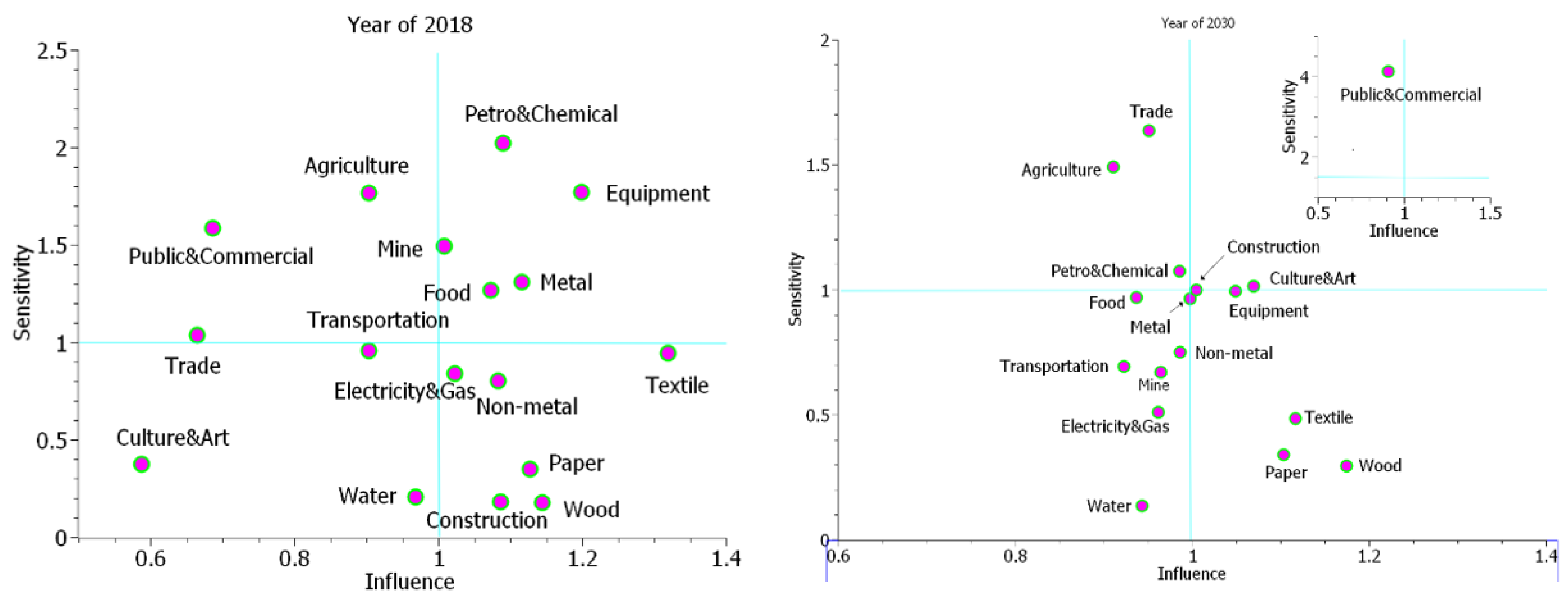
4.4. Influence and Sensitivity Coefficients

Once the coefficient of 2018 and anticipated coefficient matrix of 2030 are obtained, the influence and sensitivity coefficient can be calculated by using Formulas (9) and (10). The results are shown in

Table 2. Comparison of coefficients between 2018 and 2030.

No.	Sector	Influence Coefficient			Sensitivity Coefficient
		Year of 2018	Year of 2030 (Prediction)	Changing Trend	Year 2018	Year 2030 (Prediction)	Changing Trend
1	Agriculture, Fishery, and Forestry	0.904813799	0.911193495	↓	1.762027066	1.488778679	↓
2	Mining and Quarrying	1.009079544	0.965229629	↓	1.489040976	0.665824097	↓
3	Food product, Beverage, and Tobacco	1.07347282	0.937524512	↓	1.260593194	0.96751964	↓
4	Textile, Leather Industries	1.320953003	1.117117863	↓	0.940646051	0.481975322	↓
5	Manufacture of Wood and Wood products	1.144890402	1.17549248	↑	0.173149877	0.291590586	↑
6	Manufacture of Paper and Paper Products, Printing and Publishing	1.128036709	1.103835222	↓	0.344761535	0.337072054	↓
7	Manufacture of Industrial Chemicals and petrochemicals	1.090738039	0.986463947	↓	2.018706162	1.071174135	↓
8	Manufacture of Non-metallic Mineral Products	1.084037308	0.986846186	↓	0.795797208	0.747015255	↓
9	Basic Metal Industries	1.117413045	0.998128947	↓	1.304609116	0.960560485	↓
10	Equipment	1.199747846	1.049484139	↓	1.76799118	0.992071028	↓
11	Electricity	1.024260271	0.962016243	↓	0.832964451	0.507226756	↓
12	Water supply and waste	0.969568481	0.943859788	↓	0.201398544	0.13147807	↓
13	Construction	1.08760903	1.005504157	↓	0.17441818	0.997242957	↑
14	Wholesale and retail trade	0.665885129	0.951670374	↑	1.0317304	1.632107876	↑
15	Transportation	0.904065837	0.923489878	↑	0.95291135	0.689591594	↓
16	Commercial, public services, and others	0.687125641	0.911856852	↑	1.579653219	4.118776369	↑
17	Culture, Education, Sports, Art	0.588303097	1.070286291	↑	0.369601491	1.009995095	↑

:

As can be seen from the above table, each industry changes in a different direction. In terms of influence coefficient, 5 of the 17 sectors increased, while 12 sectors decreased. Among them, the sector of culture, education, sports, and art (No.17) increased the most, and the textile and leather industry (No.4) had the largest decline value. For the sensitivity coefficient, 5 of the 17 sectors rose while 12 sectors fell, with the fastest rise being that of commercial and public services (No.16) and the fastest decline being that of chemical and gasoline production (No.7). In comparison, there are 4 sectors with both increasing influence coefficients and sensitivity coefficients, and 12 sectors with both decreasing influence coefficients and sensitivity coefficients. Additionally, the construction sector (No.13) had a decreasing influence coefficient and increasing sensitivity coefficient, while the transportation sector (No.15) had an increasing influence coefficient and decreasing sensitivity coefficient.

As mentioned above, these two coefficients represent different importance in the economic system, so putting these sectors into a coordinate axis will present their functions more clearly, as in Figure 1 below.

As can be seen from the above figure, the number of sectors with both sensitivity and influence coefficients less than 1 increased from three in 2018 to six in 2030. At the same time, the number of sectors with both sensitivity and influence coefficients greater than 1 dropped from five in 2018 to one in 2030. The number of sectors with a sensitivity coefficient greater than 1 and an influence coefficient less than 1 increased from three in 2018 to four in 2030. The number of sectors with a sensitivity coefficient less than 1 and an influence coefficient greater than 1 decreased from six in 2018 to four in 2030.

5. Discussion and Recommendations

From the empirical analysis results, the carbon emissions in 2030 will be 12.8 billion tons. The total output value will be USD 116 trillion, showing an increase of 233% compared to the value in 2018.The prediction of China’s carbon emissions in 2030 in this paper is close to the semi-official prediction of the Chinese government and the prediction results in other literatures [38,39]. The results also show that the industry structure will be changed dramatically under the constricts of “dual goal”.

From the perspective of sector changing, the influence coefficient and sensitivity coefficient of the culture, education, and sports sector (No.17); commerce and public service sector (N.16); wholesale and retail trade sector (No.14); and manufacture of wood and wood products sector (No.5), most of which belong to tertiary industry, will be significantly enhanced. Meanwhile, the influence and sensitivity of sectors such as agriculture (No.1) and most secondary industry—including mining (No.2), food products (No.3), textile products (No.4), and so on—will show a downward trend. In fact, during recent decades in China, in accordance with the requirements of environmental protection, industry has been adjusted continuously, and the proportion of China’s tertiary industry has increased to 53.3% in 2021 compared to the value of 46.1% in 2013, which is the first time that the proportion of tertiary industry exceeded that of secondary industry [40]. The prediction results show that China’s ongoing industrial adjustment is in line with the direction of carbon emission reduction, and to achieve the 2030 carbon emission reduction goal, it must still adhere to this direction.

From the perspective of relative position in the economic system in China, all the sectors are allocated in the axis. The sectors in the top-right area are the pillar sectors; those in the top-left area and bottom-right areas are important sectors; and those in the bottom-left area are normal sectors. In 2018, there were five sectors in the pillar sector area, and most belonged to manufacturing industry, which represents that manufacturing industry played a key role in China’s economic system. However, in 2030, only one sector—the culture and art sector (No.17)—fell in this area. Regarding the important sectors that fell into the top-left area and bottom-right area, there are also some changes. For example, the electricity and gas sectors left this area.

China has been one of the biggest manufacturing countries in the world for years. China benefits greatly from this; however, this situation carries a byproduct of high carbon emissions, which pushes China to the top of the emissions list. Based on the analysis above, some measures should be taken to alleviate the pressure and reduce carbon emissions in the long run while maintaining relatively steady growth. Firstly, China must adjust its industry structure by investing in tertiary industries and reducing its manufacturing related industries gradually. Secondly, China must advance its technologies related to production activities to reduce the carbon intensity of each sector.

In addition to adjustment of investment and technological advancement, legal and market mechanisms can also be used to influence industry structure. For example, the establishment of a carbon emission permit system and a carbon emission trading market can change the emission behavior of enterprises and reduce carbon emissions [41,42]. At the same time, the implication of strict environmental protection laws and the exert of environmental taxes can drive enterprises to improve production technology. Additionally, investing in more advanced industries helps to increase labor productivity and economic growth [43,44,45].

6. Conclusions

This study adopts a linear programming input–output model and an RAS updating technique to predict the minimal carbon emission and industrial structure changing in 2030 under the constraints of “dual goal”. The research shows that most of the manufacturing sectors in China will lose their vital positions by 2030, and the service sectors will them over. This paper provides a new approach to the prediction of economic structure change and provides policy makers with practical policy recommendations. Moreover, compared to existing optimization models, since this research uses the annual updated carbon emission database and IO database, the timeliness of the prediction has been greatly improved. In the future, IA technology can be used to set up an automatic prediction program based on the yearly announced database. These are the main marginal contributions of this paper.

There are some limitations to this study. One such limitation is that the direct consumption matrix could vary in the long run, which may influence the accuracy of the results. However, this method is innovative, and as mentioned above, adjustments can be made in a timely manner based on the data which are announced every year. As a new approach to prediction on the economic structure level, it is meaningful and helpful to the government and policy makers to act in advance.

COVID-19 and the lockdown measures it brings have had an impact on global carbon emissions. In 2020, global carbon emissions dropped by 5.1% worldwide due to COVID-19, but in 2021, emissions rebounded up to an increase of 6%, showing that the impact of COVID-19 on carbon emissions is complex [46]. From China’s perspective, COVID-19 also has had an impact on China’s economy, which in turn indirectly affects China’s economic growth and carbon emissions. The prediction of this study ranges from 2018 to 2030; inevitably, COVID-19 will exert an economic-structure-changing. However COVID-19 is still ongoing and has not finished yet. Considering its lag effect, it is very important to update the prediction when the data of 2020 and 2021 are announced in the future.

References

1. United Nations Environment Programme. Emissions Gap Report 2020. Nairobi. 2020. Available online: https://www.unep.org/emissions-gap-report-2020 (accessed on 26 March 2022).
2. The State Council of China. China Releases White Paper on Climate Change Response, 28 October 2021. Available online: http://english.www.gov.cn/news/videos/202110/28/content_WS617a1072c6d0df57f98e4115.html (accessed on 10 April 2022).
3. The World Bank. World Development Indicators. Available online: https://pip.worldbank.org/country-profiles/CHN (accessed on 26 March 2022).
4. The State Council. Report on the Work of the Government. 2022. Available online: http://www.china.org.cn/chinese/2022-03/14/content_78106770.htm (accessed on 14 March 2022). (In Chinese and English).
5. Morgan, J.P. Five Questions about China’s Economy in 2022. Available online: https://www.jpmorgan.com/insights/research/china-economy-2022 (accessed on 17 March 2022).
6. European Commission; Joint Research Centre; Olivier, J.G.J.; Guizzardi, D.; Schaaf, E.; Solazzo, E.; Crippa, M.; Vignati, E.; Banja, M.; Muntean, M.; et al. GHG Emissions of All World: 2021 Report, Publications Office of the European Union, 2021. Available online: https://data.europa.eu/doi/10.2760/173513 (accessed on 16 June 2022).
7. Leontief, W.W. Quantitative Input and Output Relations in the Economic Systems of the United States. Rev. Econ. Stat. 1936, 18, 105–125. [Google Scholar] [CrossRef] [Green Version]
8. Leontief, W. An Alternative to Aggregation in Input-Output Analysis and National Accounts. Rev. Econ. Stat. 1967, 49, 412–419. [Google Scholar] [CrossRef]
9. Klinsrisuk, R.; Pechdin, W. Evidence from Thailand on Easing COVID-19’s International Travel Restrictions: An Impact on Economic Production, Household Income, and Sustainable Tourism Development. Sustainability 2022, 14, 3423. [Google Scholar] [CrossRef]
10. Choi, J.; Kim, W.; Choi, S. The Economic Effect of the Steel Industry on Sustainable Growth in China—A Focus on Input–Output Analysis. Sustainability 2022, 14, 4110. [Google Scholar] [CrossRef]
11. Allan, G.J.; Hanley, N.D.; Mcgregor, P.G.; Kim Swales, J.; Turner, K.R. Augmenting the Input–Output Framework for ‘Common Pool’ Resources: Operationalizing the Full Leontief Environmental Model. Econ. Syst. Res. 2007, 19, 1–22. [Google Scholar] [CrossRef]
12. Andrew, R.; Peters, G.P.; Lennox, J. Approximation and regional aggregation in multi-regional input-output analysis for national carbon footprint accounting. Econ. Syst. Res. 2009, 21, 311–335. [Google Scholar] [CrossRef]
13. Li, J.; Crawford-Brown, D.; Syddall, M.; Guan, D. Modeling Imbalanced Economic Recovery Following a Natural Disaster Using Input-Output Analysis. Risk Anal. 2013, 33, 908–1921. [Google Scholar] [CrossRef]
14. Elorri, I.; Rugani, B.; Rege, S.; Benetto, E.; Drouet, L.; Zachary, D.S. Combination of equilibrium models and hybrid life cycle-input–output analysis to predict the environmental impacts of energy policy scenarios. Appl. Energy 2015, 145, 234–245. [Google Scholar] [CrossRef] [Green Version]
15. Liu, X.; Moreno, B.; SaloméGarcía, A. A grey neural network and input-output combined forecasting model. Primary energy consumption forecasts in Spanish economic sectors. Energy 2016, 115, 1042–1054. [Google Scholar] [CrossRef]
16. Vogstad, K.O. Input-Output Analysis and Linear Programming. In Handbook of Input-Output Economics in Industrial Ecology; Eco-Efficiency in Industry and Science; Suh, S., Ed.; Springer: Dordrecht, The Netherlands, 2009; Volume 23. [Google Scholar] [CrossRef]
17. Wang, T.-F.; Miller, R.E. The economic impact of a transportation bottleneck: An integrated input-output and linear programming approach. Int. J. Syst. Sci. 1994, 26, 1617–1632. [Google Scholar] [CrossRef]
18. Ten Ra, T.; Steel, M.F. Revised stochastic analysis of an input–output model. Reg. Sci. Urban Econ. 1994, 24, 161–175. [Google Scholar] [CrossRef] [Green Version]
19. San Cristóbal, J.R. An environmental input-output linear programming model to reach the targets for greenhouse gas emissions set by the Kyoto protocol. Econ. Syst. Res. 2010, 22, 223–236. [Google Scholar] [CrossRef]
20. Chen, L. Identifying lowest-emission choices and environmental pareto frontiers for wastewater treatment wastewater treatment input–output model based linear programming. J. Ind. Ecol. 2011, 15, 367–380. [Google Scholar] [CrossRef]
21. Yu, K.D.; Aviso, K.B.; Promentilla, M.A.B.; Santos, R.J.; Tan, R.R. A weighted fuzzy linear programming model in economic input–output analysis: An application to risk management of energy system disruptions. Environ. Syst. Decis. 2016, 36, 183–195. [Google Scholar] [CrossRef]
22. Nguyen, H.T.; Aviso, K.B.; Le, D.Q.; Kojima, N.; Tokai, A. A linear programming input–output model for mapping low-carbon scenarios for Vietnam in 2030. Sustain. Prod. Consum. 2018, 16, 134–140. [Google Scholar] [CrossRef]
23. Kang, J.; Ng, T.S.; Su, B. Optimizing electricity mix for CO2 emissions reduction: A robust input-output linear programming model. Eur. J. Oper. Res. 2020, 287, 280–292. [Google Scholar] [CrossRef]
24. Su, Y.; Liu, X.; Ji, J.; Ma, X. Role of economic structural change in the peaking of China’s CO2 emissions: An input–output optimization model. Sci. Total Environ. 2021, 761, 143306. [Google Scholar] [CrossRef]
25. Yu, S.; Zheng, S.; Li, X.; Li, L. China can peak its energy-related carbon emissions before 2025: Evidence from industry restructuring. Energy Econ. 2018, 73, 91–107. [Google Scholar] [CrossRef]
26. Ronald, E.M.; Peter, D.B. Input–Output Analysis Foundations and Extensions, 2nd ed.; Cambridge University Press: Cambridge, UK, 2009; p. 555. [Google Scholar]
27. Stone, R. Input-Output and National Accounts; Organization for European Economic Cooperation: Paris, France, 1961. [Google Scholar]
28. Bacharach, M. Biproportional Matrices and Input-Output Change; Cambridge University Press: Cambridge, UK, 1970; p. 4. [Google Scholar]
29. Chansombat, S.; Pongcharoen, P.; Hicks, C. A mixed-integer linear programming model for integrated production and preventive maintenance scheduling in the capital goods industry. Int. J. Prod. Res. 2019, 57, 61–82. [Google Scholar] [CrossRef]
30. Emeç, Ş.; Akkaya, G. Developing a new optimization energy model using fuzzy linear programming. J. Intell. Fuzzy Syst. 2021, 40, 9529–9542. [Google Scholar] [CrossRef]
31. Shan, Y.; Guan, D.; Zheng, H.; Ou, J.; Li, Y.; Meng, J.; Mi, Z.; Liu, Z.; Zhang, Q. China CO2 Emission Accounts 1997–2015. 2018. Available online: https://www.nature.com/articles/sdata2017201 (accessed on 16 January 2018).
32. Shan, Y.; Huang, Q.; Guan, D.; Hubacek, K. China CO2 Emission Accounts 2016–2017. Scientific Data. 2020. Available online: https://www.nature.com/articles/s41597-020-0393-y (accessed on 13 February 2022).
33. Guan, Y.; Shan, Y.; Huang, Q.; Chen, H.; Wang, D.; Hubacek, K. Assessment to China’s recent emission pattern shifts. Earth’s Future 2021, 9, e2021EF002241. [Google Scholar] [CrossRef]
34. OECD. Input-Output Table. 2021. Available online: https://stats.oecd.org/Index.aspx?DataSetCode=IOTS_2021 (accessed on 30 April 2022).
35. Xu, L.; Chen, N.; Chen, Z. Will China make a difference in its carbon intensity reduction targets by 2020 and 2030? Appl. Energy 2017, 203, 874–882. [Google Scholar] [CrossRef]
36. Cui, L.; Li, R.; Song, M.; Zhu, L. Can China achieve its 2030 energy development targets by fulfilling carbon intensity reduction commitments? Energy Econ. 2019, 83, 61–73. [Google Scholar] [CrossRef]
37. Li, P.; Ouyang, Y. Quantifying the role of technical progress towards China’s 2030 carbon intensity target. J. Environ. Plan. Manag. 2021, 64, 379–398. [Google Scholar] [CrossRef]
38. International Energy Agency (IEA). An Energy Sector Roadmap to Carbon Neutrality in China. Available online: https://www.iea.org/reports/an-energy-sector-roadmap-to-carbon-neutrality-in-china/executive-summary (accessed on 20 January 2022).
39. Sun, Z.; Liu, Y.; Yu, Y. China’s carbon emission peak pre-2030: Exploring multi-scenario optimal low-carbon behaviors for China’s regions. J. Clean. Prod. 2019, 231, 963–979. [Google Scholar] [CrossRef]
40. Statistical Communiqué of the People’s Republic of China on National Economic and Social Development in 2021. China National Bureau of Statistics. Available online: https://www.stats.gov.cn/tjsj/zxfb/202202/t20220227_1827960.html (accessed on 28 February 2022).
41. Hamaguchi, Y. Polluting firms’ location choices and pollution havens in an R&D-based growth model for an international emissions trading market. J. Int. Trade Econ. Dev. 2021, 30, 625–642. [Google Scholar] [CrossRef]
42. Hamaguchi, Y. Positive effect of pollution permits in a variety expansion model with social status preference. Manch. Sch. 2019, 87, 591–606. [Google Scholar] [CrossRef]
43. Nakada, M. Does Environmental Policy Necessarily Discourage Growth? J. Econ. 2004, 81, 249–275. [Google Scholar] [CrossRef]
44. Grimaud, A.; Tournemaine, F. Why can an environmental policy tax promote growth through the channel of education? Ecol. Econ. 2007, 62, 27–36. [Google Scholar] [CrossRef] [Green Version]
45. Nakada, M. Environmental Tax Reform and Growth: Income Tax Cuts or Profits Tax Reduction. Environ. Resour. Econ. 2010, 47, 549–565. [Google Scholar] [CrossRef]
46. International Energy Agency (IEA). Global Energy Review: CO2 Emissions in 2021. Available online: https://www.iea.org/reports/global-energy-review-co2-emissions-in-2021-2 (accessed on 31 March 2022).
Figure 1. The changing positions of sectors in 2018 and 2030.
Sustainability 14 09336 g001