Prediction Liquidated Damages via Ensemble Machine Learning Model: Towards Sustainable Highway Construction Projects

Abstract

Highway construction projects are important for financial and social development in the United States. Such types of construction are usually accompanied by construction delay, causing liquidated damages ($LDs$) as a contractual provision are vital in construction agreements. Accurate quantification of $LDs$ is essential for contract parties to avoid legal disputes and unfair provisions due to the lack of appropriate documentation. This paper effort sought to develop an ensemble machine learning technique ($EMLT$) that combines algorithms of the Extreme Gradient Boosting ($XGBoost)$, Categorical Boosting ($CatBoost$), k-Nearest Neighbor ($kNN$), Light Gradient Boosting Machine ($LightGBM$), Artificial Neural Network ($ANN$), and Decision Tree ($DT$) for the prediction of $LDs$ in highway construction projects. Key attributes are identified and examined to predict the interrelated correlations among the influential features to develop accurate forecast models to assess the impact of each delay factor. Various machine-learning-based models were developed, where the different modeling outputs were analyzed and compared. Four performance matrices such as Root Mean Square Error ($RMSE$), Mean Absolute Error ($MAE$), Mean Absolute Percentage Error ($MAPE$), and Coefficient of Determination ($R^2$) were used to assess and evaluate the accuracy of the implemented machine learning ($ML$) algorithms. The prediction outputs implied that the developed EMLT model has shown better performance compared to other ML-based models, where it has the highest accuracy of 0.997, compared to the DT, kNN, CatBoost, XGBoost, LightGBM, and ANN with an accuracy of 0.989, 0.988, 0.986, 0.975, 0.873, and 0.689, respectively. Thus, the findings of this research designate that the EMLT model can be used as an effective administrative decision adding tool for forecasting the $LDs$. As a result, this paper emphasizes ML’s potential to aid in the advancement of computerization as a comprehensible subject of investigation within highway building projects.

1. Introduction

Highway facilities are a significant transportation mode for passengers and goods. For instance, the United States has one of the most sophisticated highway networks, spanning 1.3 million miles. Highway utilization has progressively augmented over the years with the development in connectivity between counties within the state. More than 343,600 thousand daily vehicle miles traveled in 2019 compared with 296,263 thousand miles in 2014 [1].

It is indispensable for highway project contract parties to ensure timely construction within the constricted accomplishment period. Unfortunately, though, construction activities regularly interfere with traffic disturbances from detours and lane closings. Although the US transportation department and the other involved parties seem to distinguish that traffic interferences are inevitable in construction projects, their influences on project delivery can still be controlled and minimalized.

Thus, the $LDs$ are considered reasonable reimbursement for the project owner to ensure the tangible damages that probably will be demanded through legalized arrangements for construction completion beyond the contractual project duration. In addition, many aspects (i.e., environment, public mobility, economy, access, and safety) are affected by the transportation project’s duration [2]. However, the planning stage for estimating the construction time and all relevant development stages had not received sufficient attention [3]. Using linear regression modeling, a study has offered a proposed model to handle this issue with three features to estimate the highway project duration [4]. Moreover, planar flow-based variational auto-encoder prediction model has been proposed to decrease the data bias and overfitting [5]. In the same vine, $XGBoost$ technique was applied to enhance the driving evaluation and risk prediction, by selecting the most important related features [6].

Claims management is a critical need for construction project success [7], especially in large and complex projects (i.e., megaprojects) [8,9]. Therefore, claim management performance criteria have been proposed to enhance the claiming management process positively. In addition, interviews have been conducted to enhance the efficiency of claims management. As a result, there is an urgent need to monitor the additional cost confirmed by project agents and $LDs$ issues [10]. $LDs$ is considered a significant feature in managing material procurement and storage [11].

Contract parties specify a pre-evaluated quantity of damage documented within the contract itself. Such measures are critical to comprise a contractual procedure instigated to recover these additional expenditures from the contractor as an alternative to actual damages [12,13]. The concurrent delay caused by subcontractors themselves or between the main contractor and other subcontractors was discussed. How to logically distribute these damages between contractors and sub-contractors in terms of liability [14]. Alternatives to the financing process were addressed in the construction project to effectively reduce financing expenditures and avert $LDs$ using the cash flow prediction model [15]. Project delay can lead to an increase in the overall project cost due to the $LDs$ [16,17].

A comprehensive analysis of policies and laws was undertaken by considering several relevant aspects (i.e., $LDs$, conflict resolution, time extension issues, change orders, and circumstance site conditions) to compare the $US$ federal acquisition regulation (and the Saudi public works contract from an international contracting perspective. This study provides the literature with integrated insight to properly understand and reduce potential risks once large contractors engage with international contracts [18]. A comprehensive survey and targeted interviews were conducted considering the $LDs$ effect for the investigation of all possible alternative highway contracting using Department of Transportation $\left(DOT\right)$ data [19]. Twenty-three private–public partnerships were examined for all potential conflicts of interest regarding public sector authority and franchisor empowerment in United States highway projects. The study shows various techniques have been applied to observe concessionaire behavior rather than empowering them in the public-private partnership [20].

In general, the $LDs$ can be thought of as accurate delay compensation fees that must be paid to the owner [21,22]. The $LDs$ that can be afforded by insurance companies in terms of predictable loss have been estimated using a case study. However, the estimated error in determining the $LDs$ was significantly high when applying this estimate to other cases where they had just established their model by adopting only one case study. Thus, this is not adequate for inclusive use [23]. For example, the I-95 express lanes project, the $LDs$ consequence has been illustrated using (VDOT 2012); The government has the authority to levy USD 5000 in $LDs$ for each day that the officially declared final decision for project completion is not released [24].

Highway construction projects normally face delays in its delivery. Such wasted time significantly affects the projects’ sustainability. As it has ripple impacts on the main project objective functions (i.e., time, quality, safety, cost, and combined $LDs$). In such cases, having an accurate $LDs$ prediction is vital for decision makers, where prospective conflicts amongst stakeholders can be avoided. Thus, a comprehensive model that considers all compelling circumstances and constraints is critically required to adapt with the construction project dynamic situations (i.e., generic prediction model). In the related model available in the literature, the actual damage is estimated, which may be much greater or less than the liquidated amount written in the relevant contract clause. To this end, few papers have investigated the $LDs$ prediction. However, to the best of the authors’ knowledge, a limited number of ML-based $LDs$ prediction models are available in the literature. Such investigations have not provided a well-defined and described analysis of the forecasting process, where only a few influential attributes were considered, and preliminary prediction tools were employed. Accordingly, the need to estimate the actual liquidated amount has become a critical issue that must be addressed in construction projects.

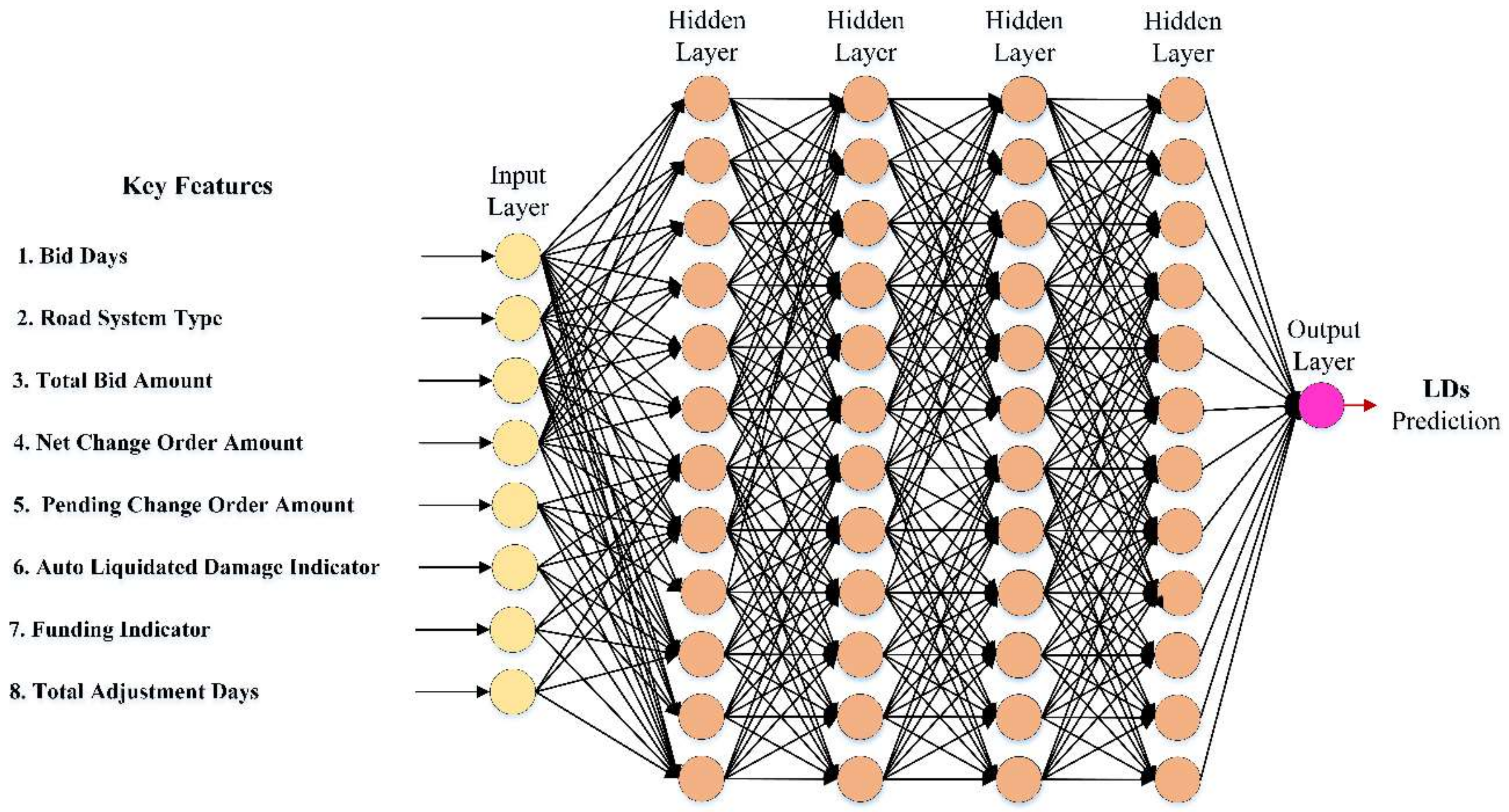
The current study creates a combined ML-based forecasting models for the prediction of $LDs$. Datasets developed during a 15-year data gathering procedure for hundreds of highway building projects collected on their contractual $LDs$ were used for training and testing. According to the recent research available within the literature and using up-to-date pre- and post-processing techniques, the most influential attributes that affect the $LDs$ prediction were chosen and defined. These factors are the net change order amount, bid days, total bid amount, road system type, auto liquidated damage indicator, pending change order amount, total adjustment days, and funding indicator. Using a complex assembled model and being generic, while considering all influential factors provide the proposed model with a step forward in the $LDs$ prediction arena. Moreover, the current study findings can be incorporated into broader ongoing research to offer a decision support tool for modernizing the$LDs$ estimation strategies worldwide.

2. $LDs$ Prediction Methodology

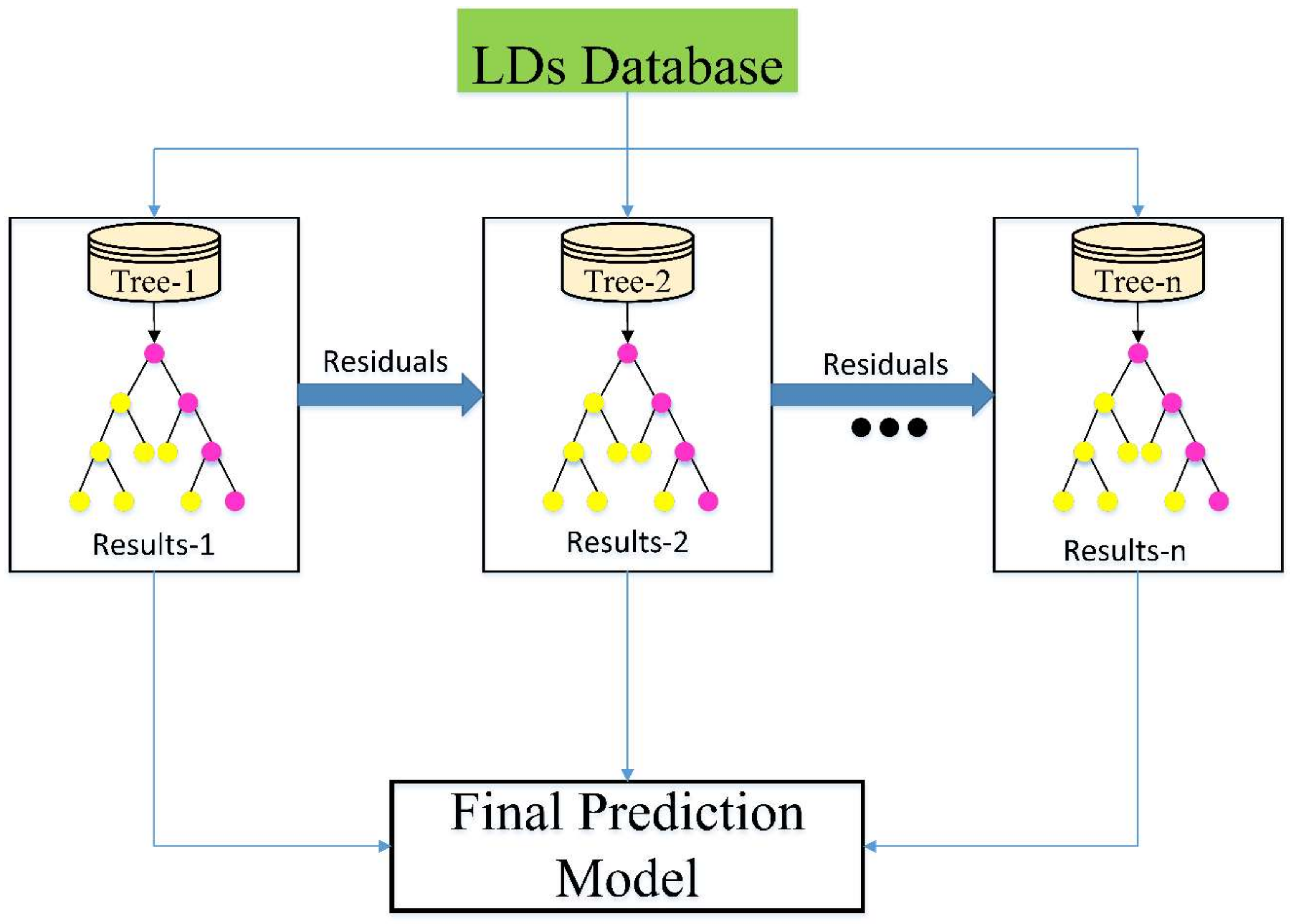
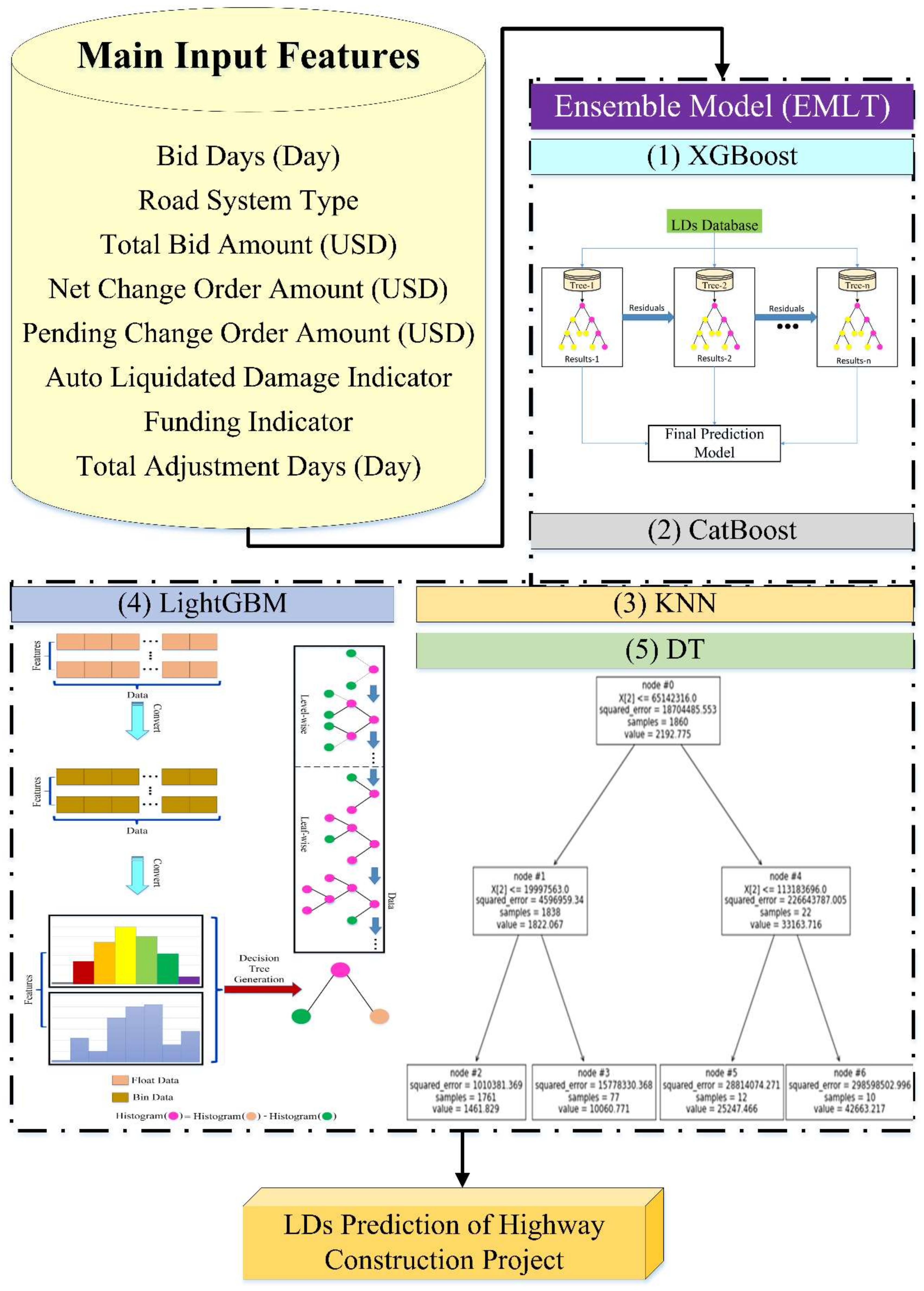
The current research paper is structured as follows. First, the latest research efforts related to $LDs$ prediction and ML-based forecasting models related to the literature are comprehensively illustrated. Then, the data collection, processing phases, and critical attributes considered in $LDs$ predictions were illustrated. In addition, the research methodology is presented, where various utilized ML techniques (i.e., XGBoost, CatBoost, kNN, LightGBM, ANN, DT) are explained and then combined. After that, various modeling results are presented and thoroughly discussed, where prediction accuracy is evaluated and compared using several performance indecencies (i.e., $MAPE$, $RMSE$, $MAE$, $R^2$). These evaluation metrics were computed to assess the proposed models’ efficiency and validity. The coefficient of determination $R^2$ embodies the precision of the forecast. Thus, for R² closer to one, additional forecast precision is acquired. The $MAPE$, the $RMSE$, and the $MAE$ are standard measures to assess the prediction accuracy with continuous dependent attributes, where they offer awareness about the forecast’s potential errors. Finally, the research conclusion along with future research recommendations are listed. The developed prediction models showed high accuracy with distinguished capabilities for $LDs$ forecasting the highway projects. Results are anticipated to play a vital role in eradicating possible struggles amongst contract parties, particularly when decision-makers tackle different complications and challenges in assessing the actual $LDs$. 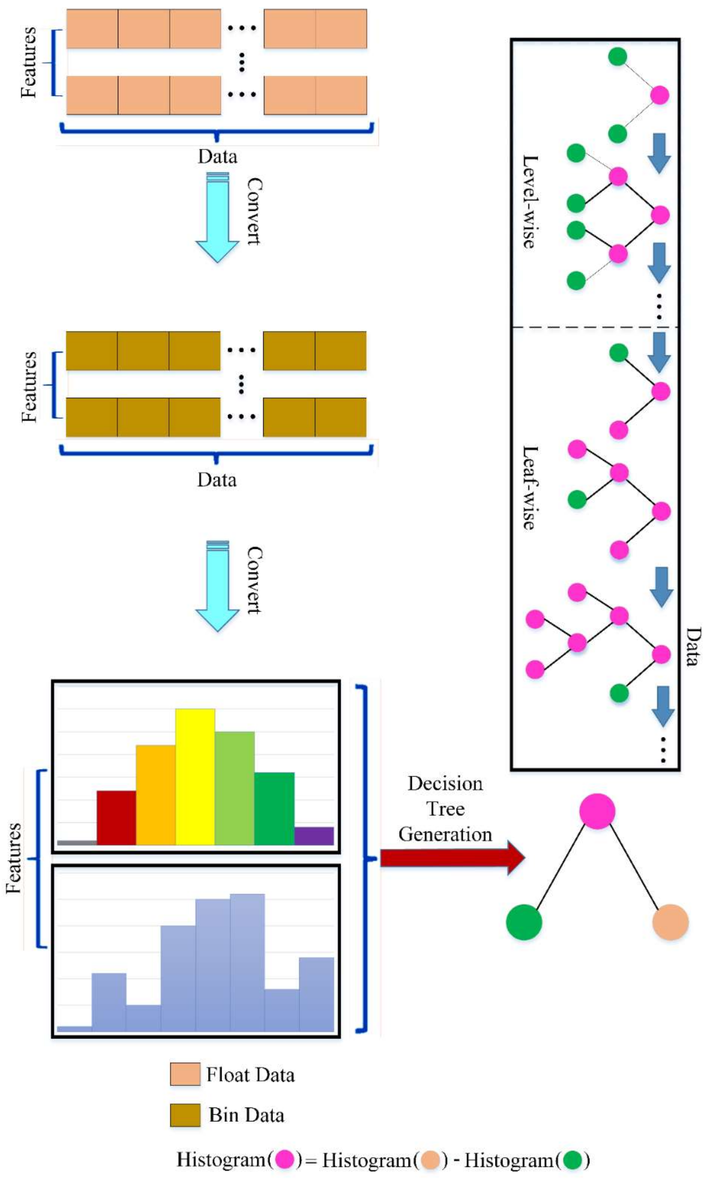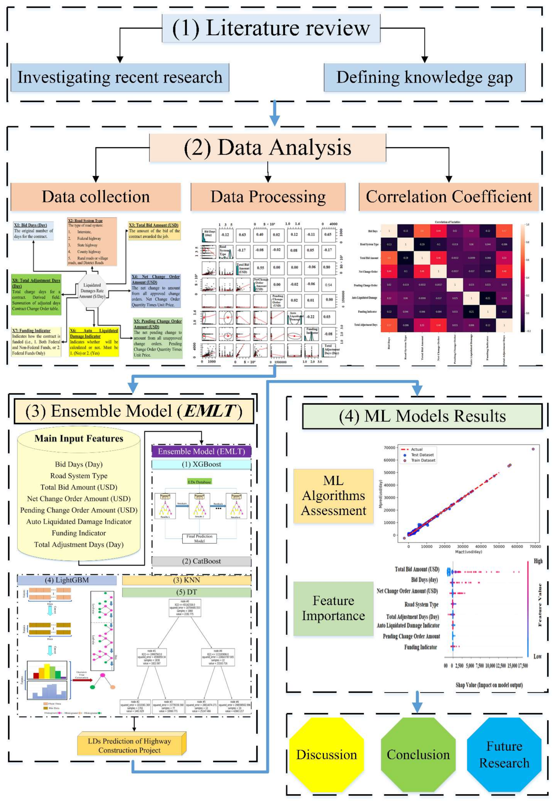For more illustrations, the methodology flowchart was carried out in Figure 1.

3. Data Processing and Analysis

3.1. Data Collection and Features Selection

The data were collected between 2006 and 2021 from the $DOT$ in Florida, US. Where the $DOT$ is a vital component for tracking the relevant dataset and the specific features of highway construction projects. For the analysis process to be more appropriate, the data was imported into $MS$ Excel. The data appear to be a promising clue that gives a proper visualization to $LDs,$ which is considered a critical factor that undergoes the project’s stakeholders to tense. The gathered data was related to the major categories of the road systems such as federal highway, interstate, county highway, state highway, rural roads, district roads, and village roads.

The gathered data provides a clue to visualize the projects’ variables and their description. Data collection transformation took about 10 months to ensure that the accumulated datasets were appropriate and representative of the $ML$ models’ technique. The study factors of $LDs$ were represented by the main attributes needed to improve the usefulness and efficiency of the developed model.

Feature selection is used to identify the most important inputs or attributes that will affect model prediction. This strategy is necessary for the success of the study, and it is an important aspect of ML to assure the creation of highly linked features [25,26]. Feature selection reduces the number of input variables to those that are deemed to be most essential to the accuracy of the prediction model. The most influential elements have been picked to launch the $LDs$ prediction models based on common information, the available literature, DOT requirements, and construction project professionals. The crucial factors were considered (i.e., net change order amount, bid days, total bid amount, road system type, auto liquidated damage indicator, pending change order amount, total adjustment days, and funding indicator).

$LDs$ are determined by several interconnected elements that have a latent influence on their value. Thus, during the prediction process itself, the feature importance is estimated and the models’ priorities from a factor selection point of view are updated accordingly. To consider the integral integrated relationship form algorithms, all LD properties must be fully identified to enable appropriate collection. To match the model input or enhance analytical precision, any features demand a transformation step. The model gets more generic and simpler by utilizing fewer functions, boosting its accuracy. Some associated features have been picked to begin the $LDs$ prediction model based on common information, the available literature, and professionals in building projects. Furthermore, a wrapper approach (backward elimination) selected the relevant feature by using its performance as an assessment criterion. Where an iterative procedure is used to reduce the model’s lowest performing features until the total accuracy of the model reaches an acceptable range [27]. The p-value is the performance parameter utilized in this study to evaluate feature performance, and features with a p-value of 0.05 or less are deleted. These variables play a significant role in the estimation process of $LDs$ of road projects. 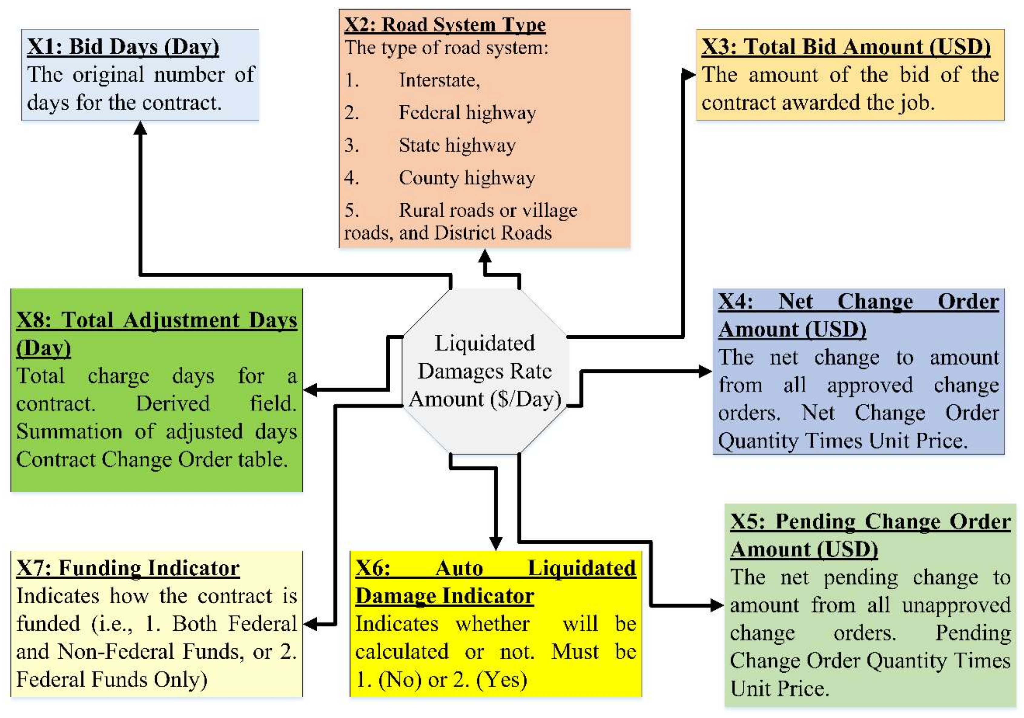Figure 2 shows the description of the eight influential dependents ($X1$ to $X8$) and one independent feature ($Y$).

3.2. Data Pre-Processing

Pre-processing the data is a crucial step for managing the data before using $ML$ algorithm. This step is required due to the need for data suitable for $ML$ techniques. The data-selection process leads to choosing a key parameter for $LDs$ estimation.

Thus,

Table 1. Descriptive statistical analysis for numerical variables of $LDs$ dataset.

Descriptive Statistics	Bid Days	Total Bid Amount (USD)	Net Change Order Amount	Pending Change Order Amount	Total Adjustment Days	Liquidated Damages Rate Amount
Mean	240	4,913,469	180,628	995	55	2125
Mode	150	600,000	0	0	0	1148
Standard Deviation	239	16,495,664	1,139,190	48,564	80	4119
Kurtosis	8	225	351	2472	17	86
Skewness	3	12	16	50	3	8
$\mathit{Q}\mathbf{1}$ (25-th)	90	357,957	0	0	9	758
$\mathit{Q}\mathbf{2}$ (50-th)	160	1,126,793	0	0	26	1148
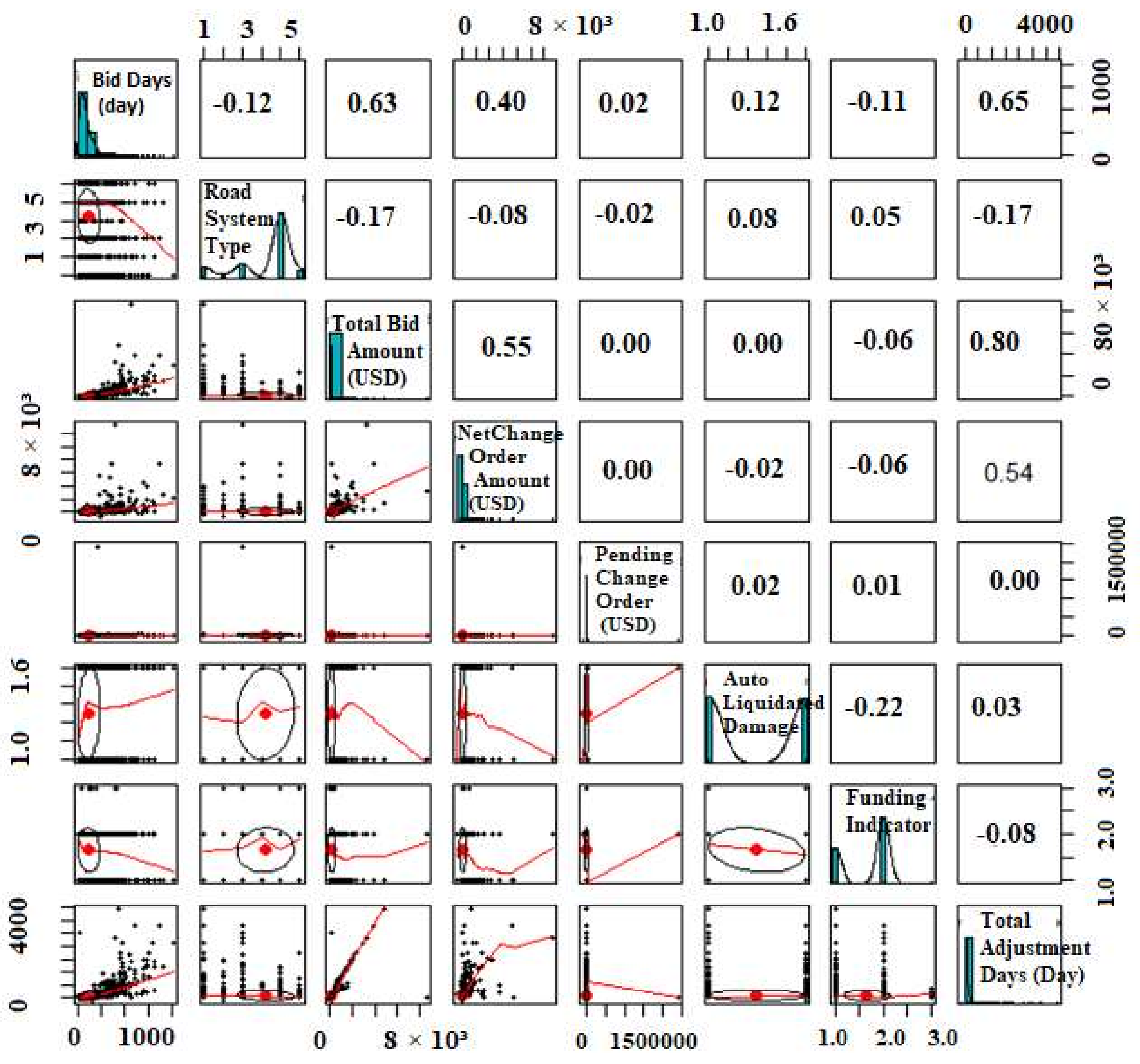
$\mathit{Q}\mathbf{3}$ (75-th)	290	3,274,002	38,419	0	67	1914

shows the numerical and independent features’ statistical measurements for the real collected data. Moreover, the scatterplot matrix for the full features is illustrated in Figure 3.

To enhance the model stability, data pre-preparation should be conducted. Several measures are needed for this process, such as data noise, normalization, outlier cleaning, standardization, conversion, and usual assortment. For pre-processing the datasets, the outliers must be excluded firstly, which is since outliers could reduce the efficiency of the model when using $ML$ techniques. Additionally, in this process, data normalization is highly required. Moreover, data filtering is conducted by employing an interquartile range to detect the extreme and outlier values. Boxplots, for example, have been chosen as a graphical method for eliminating the outliers. The “Null” indicator concept was employed for missing value representation and elimination. Consequently, a little quantity of missing data necessitated pre-processing (i.e., 8.9% of the initial database). The average and median values of pertinent attributes were used to replace the missing data points. The previously stated phases within the pre-processing step have a positive impact of the dataset readiness for the ML-based prediction phase.

After that, the transformation (from categorical feature into numerical feature) process will ensure convergence and a smooth modeling system. One-Hot Encoding is used to execute the transition [28]. Despite this, label encoding is straightforward, but algorithms can misread numeric values, since they include a hierarchical class. This ordering problem is handled through another popular alternative strategy known as ‘One-Hot Encoding’. Each category value is translated into a new column and assigned a 1 or 0 (notation for true/false) value to the column in this method. For example, the property feature categories can be encoded into numerical values, such as 100, 010, and 001 for road system type, auto liquidated damage indicator, and financing indication, respectively.

Table 2. Transforming categorical property into numerical attribute via One-Hot Encoding.

Features	Road System Type	Auto Liquidated Damage Indicator	Funding Indicator
Road System Type	1	0	0
Auto Liquidated Damage Indicator	0	1	0
Funding Indicator	0	0	1

shows how to use the One-Hot Encoding to turn the categorial property attribute into a number attribute. As a result, the entire database is converted only to contain the numerical values for all attributes.

3.3. Correlation Coefficients (CC)

The ($CC$) is used to boost the relationship between two variables by providing a linear relationship between two variables. $r\left(X,Y\right)$ is applied to calculate a numerical degree of the linear relationship between two variables $\left(X,Y\right)$ as shown in Equation (1).

$$r\left(X,Y\right)=\frac{Cov\left(X,Y\right)}{{\delta }_X{\delta }_Y}$$

(1)

where $Cov\left(X,Y\right)$, ${\delta }_{X },and {\delta }_Y$ can be calculated, as shown in Equations (2)–(4), respectively.

$$Cov\left(X,Y\right)=\frac{1}{N}{\displaystyle \sum }_{i=1}^N(x_i-\overline{x})\left(y_i-\overline{y}\right)$$

(2)

$${\delta }_X=\frac{1}{N}{\displaystyle \sum }_{i=1}^N{\left(x_i-\overline{x}\right)}^2$$

(3)

$${\delta }_Y=\frac{1}{N}{\displaystyle \sum }_{i=1}^N{\left(Y_i-\overline{Y}\right)}^2$$

(4)

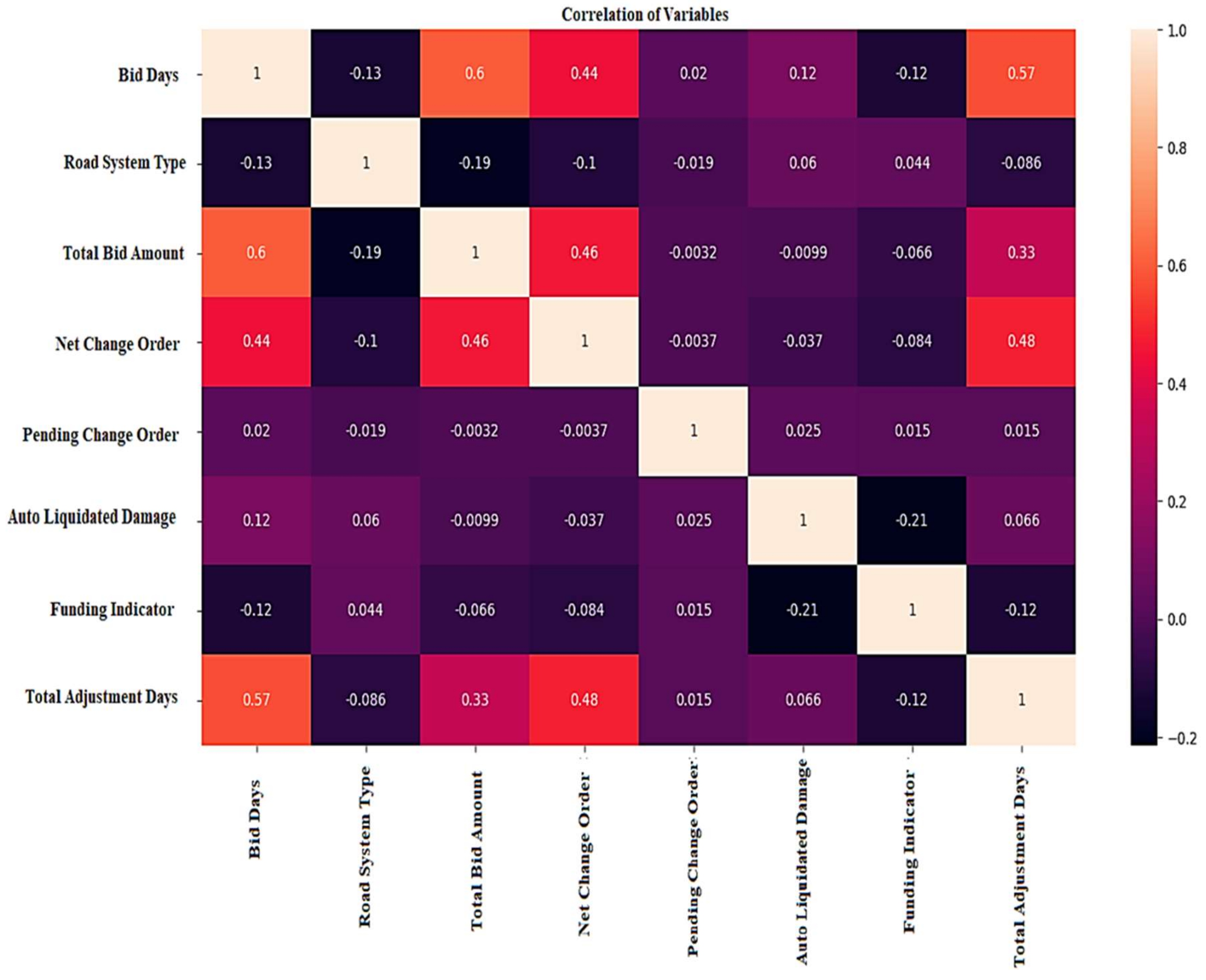
The set of the input and output of the proposed model can be represented by $i=1, 2, 3, \dots , N$for $(x_i,y_i$). In terms of Equation (1), the results will be three cases: (1) if $r\left(X,Y\right)=0$, which means no linear correlation between input $\left(X\right)$ and output $\left(Y\right)$, (2) $r\left(X,Y\right)>0$, which means a sturdy linear relationship between those variables, and (3) $r\left(X,Y\right)<0$, which means a sturdy reverse linear relationship between those variables. Thus, it is spirited to illustrate the relationship between features and assign the pairs with high positive or negative correlations. Hence, features are being defined as the Pearson coefficient into expressions; correlation rates close to one are robust and explicit correlations between the two attributes. Otherwise, the correlation values near $-1$ appear robust yet are the inverse correlation between the two features. For example, the total bid amount and bid days features have a correlation value of $0.6$, indicating that the bid days increase as the total bid amount increases. This positive correlation means a higher $LDs$ value.

Conversely, total bid amount and road system type features have a correlation estimate of $-0.19$, demonstrating the opposite impact on each other. Yet, both factors have a positive impact on the $LDs$ value. Such an illustration represents the importance of generating a heatmap that shows the interconnected relation amongst the considered attributes. Figure 4 shows the correlation between the different features.

4. ML Techniques

$ML$ techniques were employed individually to estimate the $LDs$ before being combined in this study. To evaluate the efficacy of the suggested $ML$ algorithm, training and testing processes were also carried out. The training section comprises$70\%$ of the dataset required to train the developed model, while the testing portion comprises $30\%$ of the dataset needed to carry out the testing operation. Then, 5-k-fold cross-validation was used to ensure the durability and effectiveness of the presented forecast $ML$-based models.

4.1. Extreme Gradient Boosting ($XGBoost)$

$XGBoost$ is a tree-based ensemble technique, like the random forest. $XGBoost$ also incorporates another prevalent approach known as boosting [25], in which successive trees provide greater weight to samples incorrectly predicted by earlier trees. A weighted vote of all trees produces the final forecasts [26]. $XGBoost$ acquired its name from the piece of evidence that it uses a gradient ancestry strategy to reduce loss, while adding together additional models. By combining the capabilities of these two strategies, $XGBoost$ excels at tackling supervised learning challenges. The $XGBoost$ architecture is seen in Figure 5.

4.2. Categorical Boosting ($CatBoost$)

$CatBoost$ is another boosting-based ensemble strategy that performs well with data from several categories [27]. $CatBoost$, like $XGBoost$, can handle missing numbers. $CatBoost$ distinguishes itself using symmetric trees with the same split at each level’s nodes, making it substantially faster than $XGBoost$. $CatBoost$ uses the model learned from other data to compute the residuals for each data point. As a result, each data point receives its own residual dataset. These data serve as targets, and the general model is trained over a certain number of iterations.

4.3. k-Nearest Neighbor ($kNN$)

The $kNN$ method is a simple $ML$-based technique for classification and regression [28]. The $kNN$ method searches a database for data like the current data. These newly found data are known as the current data nearest neighbors. To tackle the $LDs$ prediction problem, a similarity-based categorization might be utilized. As a result, the $LDs$ and test data are charted into a set of trajectories. Every vector characterizes $N$ dimensions for each related characteristic. A similarity measure (e.g., Euclidean distance) is calculated to decide. $kNN$ is also known as lazy learning, since it does not create a model or function in advance and instead returns the $k$ records from the training dataset that have the highest similarity to the test (i.e., query record). The class label is subsequently assigned to the query record, based on a majority vote among the chosen k records. $KNN$ is used to anticipate$LDs$ in the following way:

(a)

Locate the closest neighbors, $k$.

(b)

Ascertain the space amongst the training and query samples.

(c)

Sort out the entire training data according to distance values.

(d)

Take a majority vote on the class labels of the query record’s $k$ nearest neighbors and allocate it as a forecast value.

4.4. Light Gradient Boosting Machine ($LightGBM$)

Microsoft Research proposed $LightGBM$, a gradient-boosting $DT$ based on a decision-tree approach [29]. $LightGBM$ is a powerful approach for dealing with regression and classification issues [30]. It also uses less memory and produces more accurate forecasts. $LightGBM$ enhances training while utilizing less memory. It is based on the histogram approach and the leaf-by-leaf growth strategy of trees. Figure 6 depicts the histogram decision-tree-based approach. Figure 6 also depicts the development processes at the level and leaf levels. The level-wise growth strategy splits leave on the same layer simultaneously. Therefore, it is better to augment various strands to maintain model convolution in self-control. Furthermore, despite receiving different amounts of information, leaves on the same layer are processed the same way.

4.5. Artificial Neural Network ($ANN$)

ANN is a neural network built on a creature’s nervous process technique. The basic idea behind a neural network ($NN$) is to generate neurons or nodes that store and process datasets and connect them with artificial synapses [31]. A neural network comprises many layers of nodes that communicate with one another. The number of nodes in the input layer represents the number of attributes that reflect the assessed variables, whereas the number of neurons in the output layer represents the number of classes. The whole node takes input from the preceding layer, determines its output, and sends it to the node for the following layer as shown in Figure 7. When this procedure is repeated, the output layer nodes may provide the required outcome. The nature of the job and the amount of training data available dictate the number of neurons and hidden layers. Each neuron in the hidden and output layers was numerically connected to all the nodes in the preceding layer. The weight of the two neurons controls the signal’s amplitude that happens between the two neurons and the $ANN$’s input, hidden, and output layers.

4.6. Decision Tree ($DT$)

When used correctly, $DT$ is one of the most routinely and widely utilized $ML$ approaches, producing accurate results and being simple to understand [32]. To mention a few applications, $DT$ has been used successfully in character recognition, radar signal categorization, medical diagnosis, remote sensing, voice recognition, and expert systems. Developing a model aims to anticipate the target variable value using decision-making rules derived from data properties. The inputted datasets divide the $LDs$ data into subsets, and the procedure must be repeated for each subset. For example, a new dataset is required to compare a root node with a categorization statute that follows the route from the root to the leaf. This leaf depicts the predicted state of the output characteristic. Figure 8 depicts a schematic depiction of the $DT$, a specific form of algorithm representing the $ML$ model, using a tree-like scheme.

4.7. Ensemble Model ($EMLT)$

The $EMLT$ model was used to improve machine learning results (outcomes) by merging several models, as shown in Figure 9. Compared to a single model, this strategy enables a better predictive model. Voting ensemble, or voting classifier, was used to aggregate predictions from different machine learning algorithms ($XGBoost$, $CatBoost$, $kNN$, $LightGBM$, $DT$) to create more accurate classifiers by combining less accurate ones. It generates a strong unique learner to address regression and classification issues in the field of machine learning [33]. As a result, the combination can supplement the separate classifiers’ failures on various regions of the input space. Thus, the ensemble model’s primary principle is to mix numerous base learners in generating the final answer rather than depending on a single model [34]. A voting ensemble calculates the average of numerous other learners in regression situations (regressor). In general, regressor ensembles strategies optimize regression issues by combining the objectives using weighted average. The ensemble output ($\widehat{y_j}$) is written in Equation (5).

$$\widehat{y_j}={\displaystyle \sum }_i^k{\omega }_i{\lambda }_{ij} \left(1\right)$$

(5)

where $k$ is number of learners, ${\omega }_i$defines the weight of the ith regressor, ${\lambda }_{ij}$ defines the ith regressor yield related to the training sample.

The voting-averaged ensemble algorithm merges the outcomes in the subsequent phases:

• Categorizing: the regressor outcome ${\lambda }_j={\left({\lambda }_{1j},{\lambda }_{2j},\dots ..{\lambda }_{kj}\right)}^T$ can be split into $c$classes $\left(S_{jn}\right)\dots \left(n=1,2,\dots .c\right)$ corresponding to various approaches (e.g., ($S_{j1},S_{j2},\dots ..S_{jc})=Classifying\left({\lambda }_j\right))$.
• Voting: corresponding to the majority voting, the $\stackrel{̿}{n}-th$ class is the leader class, such as $S_{j\stackrel{̿}{n}}=$ ($S_{j1},S_{j2},\dots ..S_{jc})$.
• Averaging: the weighted average of the $\stackrel{̿}{n}-\mathrm{th}$ class is measured as the ensemble outcome equal to the ith sample (e.g., $\widehat{y_j}=$ Averaging $S_{j\stackrel{̿}{n}}$).

5. Result and Discussion

The assessment metric was used to examine the adequacy of the suggested model. It is vital to assess the efficacy and prognostic capacity of the developed model after evaluating the primary model assumptions. As indicated in

Table 3. The arithmetic formula for performance metrics.

Performance Metrics	Equation	Symbol Definition
$\mathit{M}\mathit{A}\mathit{E}$	$\frac{1}{m}{\displaystyle {\displaystyle \sum }_{i=1}^m}\left|Y_i-\overline{Y_i}\right|$	$Y_i$: actual (measured) values of the $LDs$ $\overline{Y_i}:$forecasted outcome $\overline{Y:}$ mean of the $Y_i$ $m$: number of the datasets utilized
$\mathit{R}\mathit{M}\mathit{S}\mathit{E}$	$\sqrt{\frac{1}{m}{\displaystyle {\displaystyle \sum }_{i=1}^m}{\left(Y_i-\overline{Y_i}\right)}^2}$
$\mathit{M}\mathit{A}\mathit{P}\mathit{E}$	$\frac{1}{m}{\displaystyle {\displaystyle \sum }_{i=1}^m}\left|\frac{Y_{i-}\overline{Y_i}}{Y_i}\right|\times 100$
${\mathit{R}}^{\mathbf{2}}$	$1-\frac{{{\displaystyle \sum }}_{i=1}^m{\left(Y_i-\overline{Y_i}\right)}^2}{{{\displaystyle \sum }}_{i=1}^m{\left(Y_i-\overline{Y}\right)}^2}$

, four statistical indices ($RMSE$, $MAE$, $MAPE$, R²) were used to analyze the efficacy of the developed model quantitatively. If the R² value approaches one, and the $RMSE$, $MAE$, and $MAPE$ values approach zero, the model’s accuracy and performance will improve.

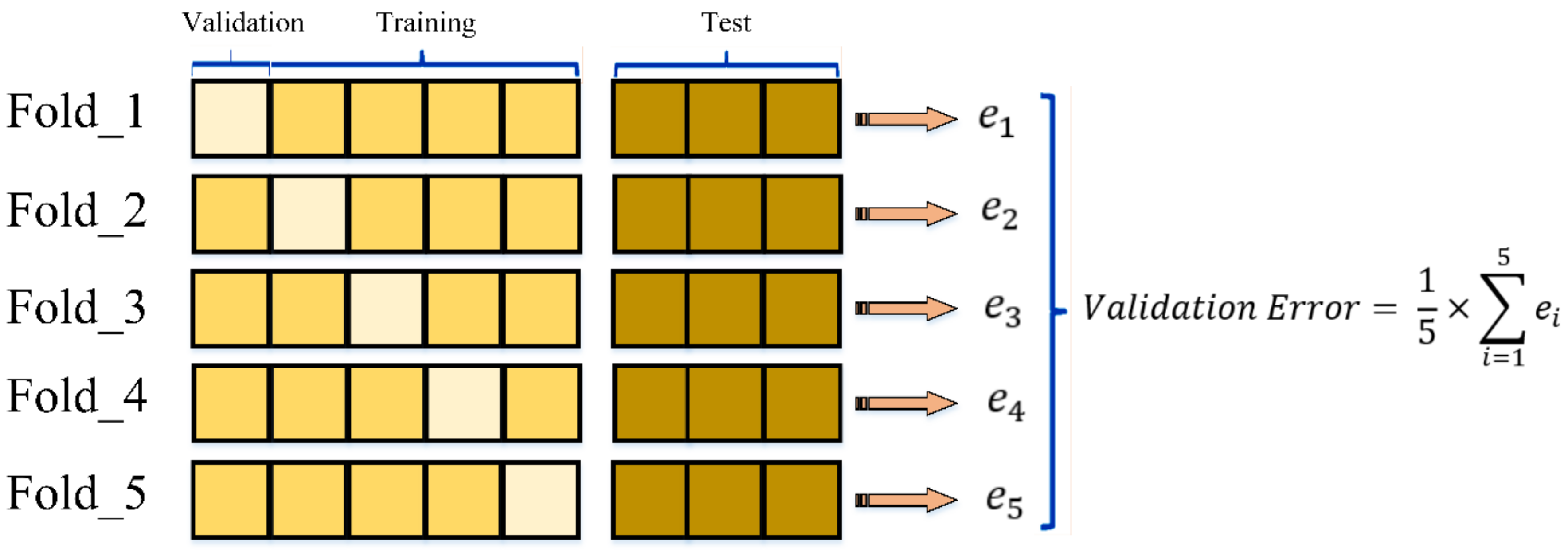
The training procedure on the $LDs$ dataset was carried out using k-fold cross-validations to assess the ensembled models’ efficacy.

Table 4. Performance of different k-folds.

k-Fold Cross-Validation	Evaluation Metrics	ML Model
		$\mathit{X}\mathit{G}\mathit{B}\mathit{o}\mathit{o}\mathit{s}\mathit{t}$	$\mathit{C}\mathit{a}\mathit{t}\mathit{B}\mathit{o}\mathit{o}\mathit{s}\mathit{t}$	$\mathit{k}\mathit{N}\mathit{N}$	$\mathit{L}\mathit{i}\mathit{g}\mathit{h}\mathit{t}\mathit{G}\mathit{B}\mathit{M}$	$\mathit{A}\mathit{N}\mathit{N}$	$\mathit{D}\mathit{T}$	$\mathit{E}\mathit{M}\mathit{L}\mathit{T}$
$\mathit{k}\mathsf{=}\mathbf{3}$	MAE	2.05	1.31	0.98	1.44	8.21	0.96	0.66
	$RMSE$	2.15	1.57	1.06	3.12	10.95	1.07	0.54
	MAPE (%)	9.3	7.4	6.8	9.5	39.6	6.7	4.9
	$R^2$	96.4	97.4	97.5	85.8	66.9	97.8	99.1
$\mathit{k}\mathsf{=}\mathbf{5}$	MAE	1.15	0.91	0.53	0.88	6.11	0.53	0.32
	MSE	2.15	1.57	1.06	3.12	10.95	1.07	0.54
	MAPE (%)	6.7	5.5	4.9	6.9	28.1	4.8	3.6
	$R^2$	97.5	98.6	98.8	87.3	68.9	98.9	99.7
$\mathit{k}\mathsf{=}\mathbf{7}$	MAE	2.11	1.39	1.02	1.49	8.66	0.99	0.70
	MSE	2.24	1.66	1.11	3.37	11.33	1.13	0.60
	MAPE (%)	10.1	7.8	7.4	10.4	40.4	7.1	4.9
	$R^2$	96.2	97.1	97.1	84.9	66.1	97.5	99.0

demonstrates a group of nonoverlapping and random partitioned folds, utilized as datasets for the training purposes of k = 3, k = 5, and k = 7, along with their related performance assessment measures. Thus, five-fold cross-validation had the greatest prediction accuracy. Figure 10 depicts the current model’s five-fold cross-validation results. It worth mentioning, as indicated in Table 4, the $ANN$ model was eliminated from the assembly process because of its low accuracy.

Table 5. Optimization hyperparameters and training times (in seconds) of the $ML$ models.

ML Models	Hyperparameters	Optimal Parameters
$\mathit{X}\mathit{G}\mathit{B}\mathit{o}\mathit{o}\mathit{s}\mathit{t}$	Number of trees	80
	Learning rate	0.1
	Mamaimum depth	5
	Fraction of columns	0.3
	Training time	24
$\mathit{C}\mathit{a}\mathit{t}\mathit{B}\mathit{o}\mathit{o}\mathit{s}\mathit{t}$	Number of iterations	100
	Mamaimum depth	2
	Training time	21
$\mathit{k}\mathit{N}\mathit{N}$	Number of neighbors	3
	Training time	32
$\mathit{L}\mathit{i}\mathit{g}\mathit{h}\mathit{t}\mathit{G}\mathit{B}\mathit{M}$	Number of trees	200
	Learning rate	0.1
	Mamaimum depth	8
	Needed leaf count	40
	Fraction of columns	0.9
	Training time	20
$\mathit{D}\mathit{T}$	Mamaimum depth	4
	Min number of samples required at leaf node	40
	Max number of leaf nodes	10
	Min number sample required for a split	5
	Training time	26
$\mathit{A}\mathit{N}\mathit{N}$	Number of neurons	15
	Batch size	32
	Epochs	50
	Number of hidden layers	2
	Activation function	$ReLU$
	Training time	41
$\mathit{E}\mathit{M}\mathit{L}\mathit{T}$	Estimators	$XGBoost$, $CatBoost$, $kNN$, $LightGBM,$ and $DT$
	Training time	51

shows how the proposed ML algorithms utilized in this work must adjust their hyperparameters to determine the needed time to train the dataset. Herein, such hyperparameters are to be changed based on the actual dataset. The order in which these hyperparameters were optimized was dictated by their reciprocal interaction and the relevance of their effect on the ML model. The $LightGBM$ was also the quickest model, taking $20$ s, whereas the $EMLT$ took $51$ s. As a result, the $LightGBM$ was around 0.5 min quicker than the EMLT. Even though, the $EMLT$ was slower than the $LightGBM$ it has provided a superior prediction accuracy.

5.1. ML Models of $LDs$ Prediction Results

This paper intends to comprehensively compare the efficacy of the state-of-the-art $ML$ algorithms (i.e., $XGBoost$, $CatBoost$, $kNN$, $GBM$,$ANN, DT$) with $EMLT$ to predict the $LDs$. Various evaluation metrics (i.e., $MAE$, $RMSE$, $MAPE$, $R^2$) checked the model’s comparisons to investigate the prediction capability of the developed $ML$ models.

The previously described performance measures are calculated and given in

Table 6. Evaluation metrics for $LDs$ prediction.

Prediction Models	Training Results				Testing Results
	${\mathit{R}}^2\left(\mathit{\%}\right)$	$\mathit{M}\mathit{A}\mathit{E}$	$\mathit{R}\mathit{M}\mathit{S}\mathit{E}$	$\mathit{M}\mathit{A}\mathit{P}\mathit{E}\left(\mathit{\%}\right)$	${\mathit{R}}^2\left(\mathit{\%}\right)$	$\mathit{M}\mathit{A}\mathit{E}$	$\mathit{R}\mathit{M}\mathit{S}\mathit{E}$	$\mathit{M}\mathit{A}\mathit{P}\mathit{E}\left(\mathit{\%}\right)$
$\mathit{X}\mathit{G}\mathit{B}\mathit{o}\mathit{o}\mathit{s}\mathit{t}$	97.5	1.15	1.23	6.7	84.4	1.25	1.73	9.6
$\mathit{C}\mathit{a}\mathit{t}\mathit{B}\mathit{o}\mathit{o}\mathit{s}\mathit{t}$	98.6	0.91	0.98	5.5	86.4	1.20	1.61	6.6
$\mathit{k}\mathit{N}\mathit{N}$	98.8	0.53	0.59	4.9	87.2	1.19	1.56	6.5
$\mathit{L}\mathit{i}\mathit{g}\mathit{h}\mathit{t}\mathit{G}\mathit{B}\mathit{M}$	87.3	0.88	2.04	6.9	78.2	1.49	2.05	10.3
$\mathit{A}\mathit{N}\mathit{N}$	68.9	6.11	7.65	28.1	59.5	6.78	8.46	20.7
$\mathit{D}\mathit{T}$	98.9	0.53	0.59	4.8	87.7	1.14	1.53	6.3
$\mathit{E}\mathit{M}\mathit{L}\mathit{T}$	99.7	0.32	0.37	3.6	95.3	1.01	1.13	4.1

for the entire model. Table 6 shows that the $EMLT$ model outperforms the single models in predictive performance (i.e., $XGBoost$, $CatBoost$, $kNN$, $LightGBM$, $ANN$, $DT$). The $CatBoost$ and $DT$ models fared similarly on the training dataset, while the $CatBoost$ model achieved better performance on the test dataset, as shown in Table 6. The $ANN$ model performed the worst on the training and test sets alike, with the lowest coefficient of determination (68.9% and 59.5% on the training and test sets, respectively) and the highest in the rest of the metrics, such as $RMSE$ (7.65 and 8.46 on the training and test datasets, respectively), as shown in Table 6. The $EMLT$ model outperformed all other developed models on the training and test phases alike, as seen by the performing measures in Table 6. The arithmetical metrics for the $EMLT$ developed model is 95.3% ($R^2$), 1.01 ($MAE$), 1.13 ($RMSE$), and 4.1% ($MAPE$) on the test dataset, as itemized in Table 6. The coefficient of determination numeric value for the $XGBoost$, $CatBoost$, $kNN$, $GBM$,$ANN$, and $DT$models was 84.4%, 86.4%, 87.2%, 78.2%, 59.5%, and 87.7%, respectively, matched to $R^2$ value of 95.3% for the $EMLT$ model developed on the test dataset, as described in Table 6. 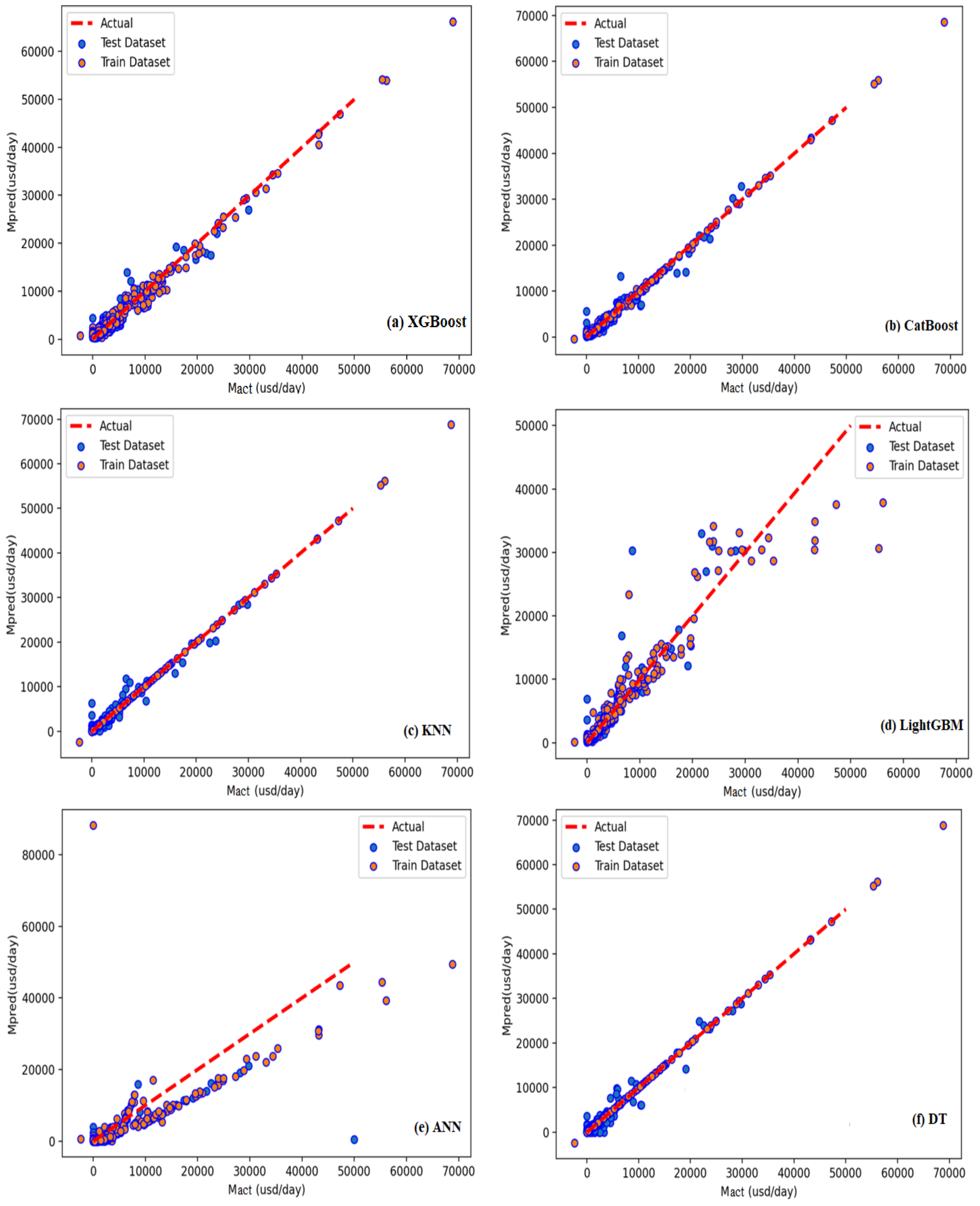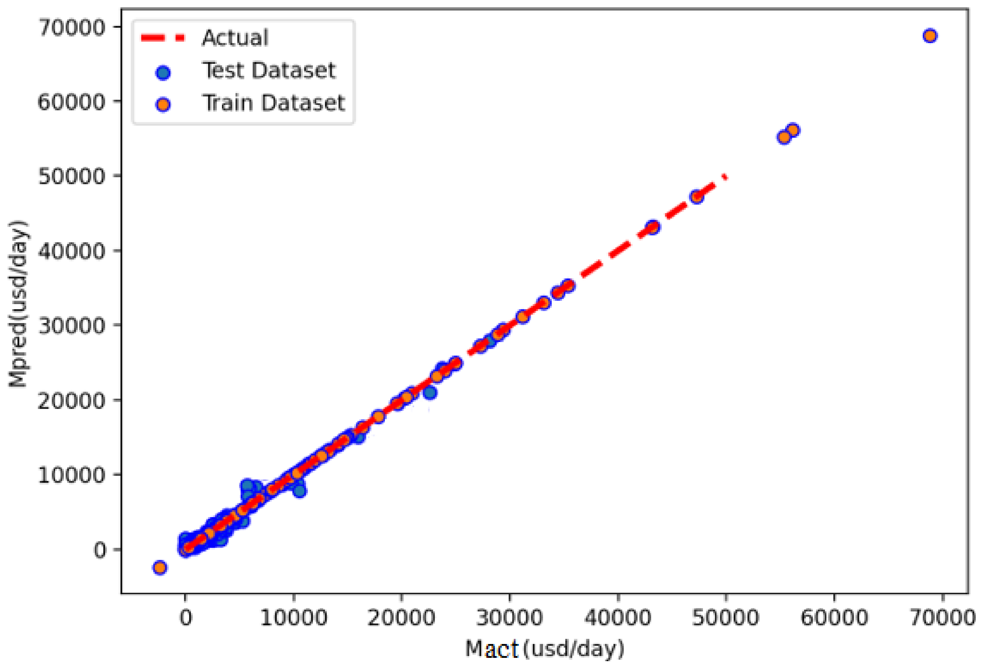Figure 11a–f and Figure 12 provide scatter plots for anticipated ($Mpred$) against actual ($Mact$) $LDs$ values, using single $ML$ and ensemble $ML$ models’ $EMLT$, respectively. Overall, the created $ML$ models ($XGBoost$, $CatBoost$, $KNN$, $DT$, $EMLT$) demonstrated a 97.5%correlation between $LDs$’ actual and projected values during the testing phase. Among the single models, $ANN$ had the lowest prognostic performance in the training and test sets, while $DT$ had the highest.

However, the $DT$ model requires improvement because its R² in the testing procedure for $LD$s prediction was 87.7%. As shown in Figure 12, the predicted value of the testing and training processes is tightly centered on the 45-degree diagonal line, which displays a complete matching among the predicted and corresponding actual values in the testing and training datasets. Furthermore, as shown in Table 6, the proposed ensemble model $EMLT$ resulted in a significant correlation between the predicted and actual, as indicated by the coefficient of determination, R² $\ge$ 95.3%, in both phases (i.e., testing and training). As a result of this discovery, the suggested ensemble model $EMLT$ successfully forecasts the $LDs$, as shown in Figure 12.

5.2. Feature’s Importance Analysis

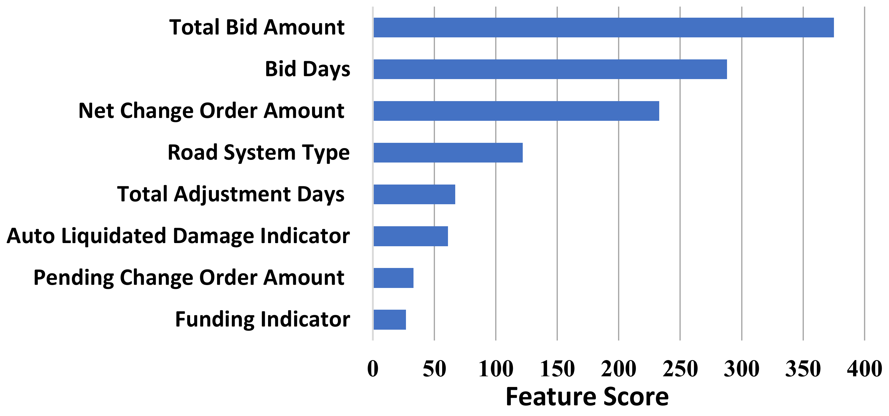
We do feature significance analysis based on the $EMLT$ after developing the $EMLT$ model with the eight features to predict $LDs$. Figure 13 depicts these traits in descending order of significance. In this part, we take the feature significance analysis a step further. The contribution of each feature to increasing the prediction performance of the overall model is referred to as feature significance. It can intuitively reflect the relevance of features and observe which characteristics significantly affect the final model, but it is hard to determine how the feature and the final forecast are related.

The total bid amount, bid days, and net change order amount are the three most significant factors, as shown in Figure 13. In contrast, the pending change order amount and financing indication are the least relevant parameters for predicting $LDs$ using the suggested $EMLT$ model. Figure 13 does not reveal whether these characteristics have positive or negative correlations with $LDs$ or whether they have other more complicated associations. 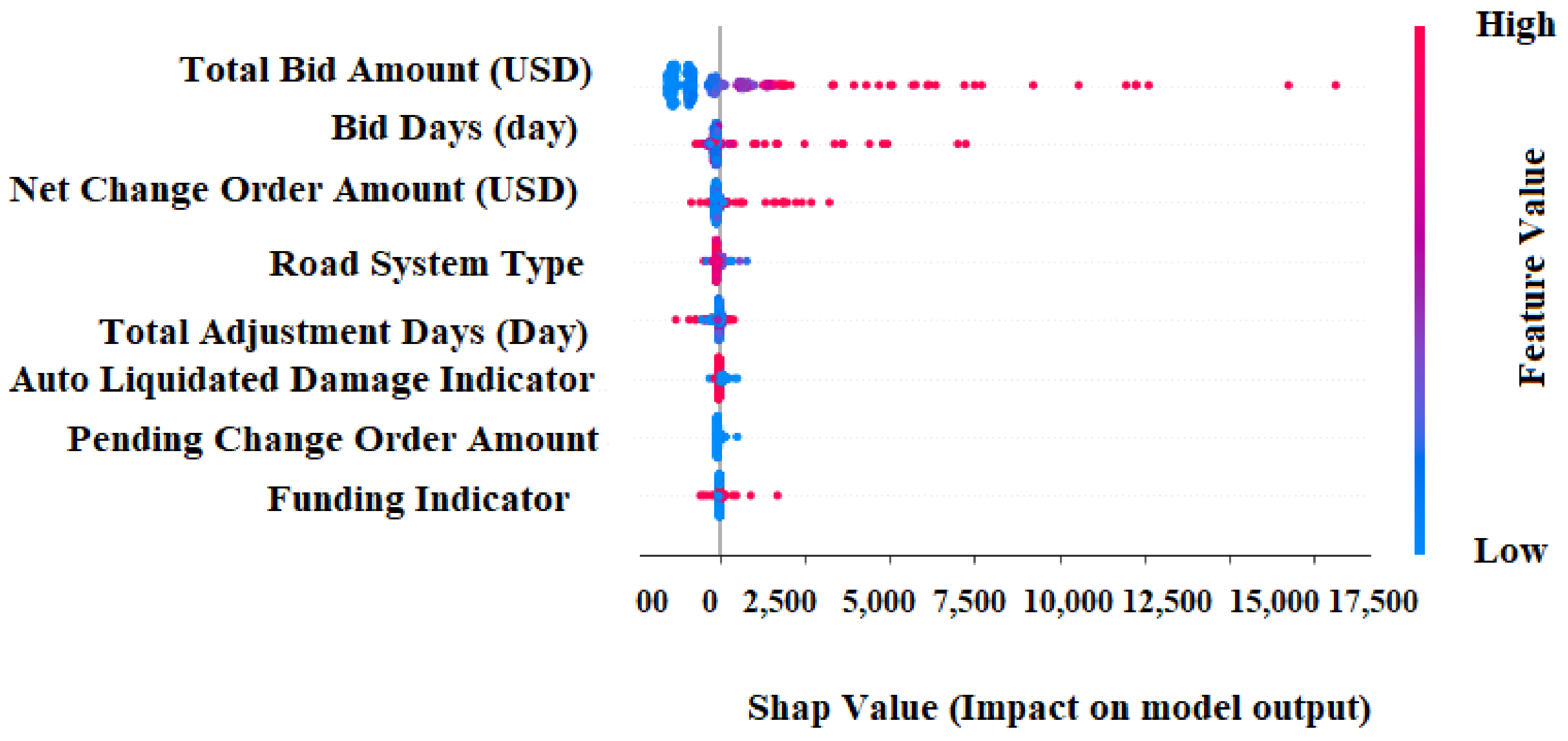Figure 14 depicts the distribution of Shapley values for every attribute throughout the whole dataset.

Each point in this diagram signifies a Shapley value for an attribute and a unique reflection in the dataset. Each dot on the x-axis indicates a Shapley value for each factor, indicating the effect of each component on the $LDs$, while the y-axis lists the factors in order of significance. The higher the value of the feature is, the redder the color, and the lower the value of the feature is, the bluer the color. We can see from Figure 14 that the total bid amount is an essential aspect, and it is largely positively connected with $LDs$.

Bid days, net change order amount, and financing indicators are also good predictors of $LDs$, so raising the values of these variables can improve $LDs$ prediction. Pending change order quantity and road system type are inversely connected with$LDs$, and the lower the values of these characteristics are, the better the model’s prediction. Other characteristics do not affect $LDs$.

During the $15$-year study period, the departments of transportation all over the $\mathrm{US}$ have collected around $3500$ distinct highway construction projects, with eight early specified characteristics to construct a model with a flexible concept to deal with all the types of factors that might arise in the future. Furthermore, the suggested model may be constructed with new road forms that must be handled. Eight road system data variables were employed as predictor factors for highway development projects to generate hybrid machine learning models to forecast the associated liquidated damages.

The modeling prediction results are intended to contribute to developing a comprehensive long-term framework, for estimating the presently enacted highway code requirements and prosecution processes enlightened by the findings of this study. As a result, the proposed model gives the scientific capability for the decision-maker to evaluate these conflicts in such a setting. Furthermore, they would be given sufficient information regarding the disagreement.

This disagreement was identified as a critical obstacle that needs to be solved to finish a motorway project. Contractors aim to reduce their expenditures due to late task execution by keeping the owner responsible as the principal cause of late delivery/task execution. However, the expected income might change at any time. Whereas, if the contractors are not entirely aware of the expenditures and time compensation, the business may go bankrupt due to $LDs$. According to contract law, the time required to finish a highway project must already be established. Therefore, contractors would be held accountable for such a delay. This approach was created to assist decision-makers in dealing with any $LDs$ difficulties that significantly impede project progress. Thus, it is imperative to develop technological and research-based tools (e.g., machine and deep learning, optimization, and decision support tools) that can be practically used to pave the road towards creating comprehensive guidelines and policies to minimize the financial claims in the construction industry and foster the automation in the construction management arena [35,36,37,38,39,40,41,42,43,44,45,46].

6. Conclusions

The current study proposed six modified 𝑀𝐿 models for forecasting 𝐿𝐷𝑠, while a hybrid model was developed via a systematic combination of the crated individual models adopted with the $EMLT$ model. The obtained results from each individual ML model can be classified as satisfactory, i.e., the EMLT had an accuracy of 0.997, compared to the DT, kNN, CatBoost, XGBoost, and LightGBM, with an accuracy of 0.989, 0.988, 0.986, 0.975, and 0.873, respectively. However, to reach maximum prediction accuracy, it was found that the developed model’s fusion is vital to enhance the forecasting results. According to the analysis results, the most critical eight independent indicators for forecasting $LDs$ are road system type, bid days, finance indicator, total bid amount, net change order amount, auto liquidated damage indicator, total adjustment days, and pending change order amount. Nevertheless, the four most significant attributes were the overall bid amount, bid days, net change order amount, and type of road system.

Since $LDs$ are often calculated as a percentage of the entire venture expense, the impact of the total bid amount may be explained. As a result, the $LDs$ are likely to rise as the entire project cost rises. In addition, the circumstance clarifies the impact of bid days that venture length has a significant impact on $LDs$, since projects with extended periods have higher costs. Additionally, the amount of the net change order plays a vital role in determining the $LDs$. Thus, the net change order amount has a positive relationship with the $LDs$. This can be explained by the fact that contractors gain high revenues from the projects’ change orders, without considering their impact of the project timeline. Thus, more change orders are expected to cause extensive delays that are associated with high values of the $LDs$. Ultimately, the impact of the type of road system may be clarified by the fact that the highway system represents an essential part in establishing the regulations and guidelines that the organization that supports the project implements. Furthermore, federal requirements must ensue when the venture is a federal or interstate road, whereas state standards must be observed for state and county roads. On the other hand, the total adjustment days might not be utilized to forecast $LDs$ since some of these modifications are the consequences of change orders according to the owner’s specifications, and developers are not held accountable for delays caused by the owner’s specifications. Consequently, the outcomes of such requests are very uncertain. Moreover, the auto liquidated damage indicator, funding indicator, and pending change order amount have minimal impact of the $LDs$ prediction process.

A rudimentary $EMLT$ model improved the $LDs$ prediction in numerous situations. With better prediction performance matrices, the developed $EMLT$ model had outperformed each individually created model. Using the same comparison criteria, the descending order of the developed models’ accuracy is $EMLT$, $DT$, $KNN$, $CatBoost$, $XGBoost$, $LightGBM$, and $ANN$, respectively.

The proposed hybrid $LDs$ prediction model (i.e., $EMLT$) will most likely benefit decision-makers by predicting $LDs$. The managerial impact of the developed model is expected to pave the way towards broader long-term context for assessing the available enacted highway construction code requirements and prosecution processes informed by the conclusions of the current research. Consequently, the developed model provides the systematic capacity for decision and policymakers to assess these inconsistencies in such cases.

As a future research recommendation, data collection and recording procedures might be improved, as exact and comprehensive data are vital to forecasting $LDs$ correctly. In addition, more holistic prediction modeling might be conducted according to further advanced algorithms, after being fused with technological tools (e.g., Building Information Modeling ($BIM$), Digital Twin, Internet of Things ($IoT$), and Blockchain) which might be utilized to automatically forecast the liquidated damages for various types of construction projects.