Nexus between Housing Price and Magnitude of Pollution: Evidence from the Panel of Some High- and-Low Polluting Cities of the World

Abstract

With the growing environmental pollution and adverse climatic conditions, it is now a globally vibrant topic whether housing prices should be associated with the quality of the environment in a particular region. From the microeconomic approach to environmental economics, it is proposed that property prices in any region should be associated with the environmental quality-the concept of hedonic pricing. A negative association between low magnitudes of pollution and high house prices is a precondition to achieving the aim of sustainable development. The study thus starts with the objective of investigating whether there are long-term relations and short-term dynamics between the magnitudes of pollution and house price in the panel of the world’s high-polluting and low-polluting cities for the period of 2012–2021 across 30 cities. Using appropriate time-series econometric procedures such as panel cointegration, panel VECM, and the Wald Test, the study arrives at the conclusion that magnitudes of pollution and house prices in the cities are cointegrated with a stable long-term relationship in all panels. Further, there are strong causal interplays in both the long- and short-term between pollution and house prices in most of the panels of the cities. Thus, policy makers should consider making proper valuations of environmental services to control pollution at the city levels first and then at global levels to reach the proposed goal of sustainable development.

1. Introduction

The Intergovernmental Panel on Climate Change (IPCC) [1] first raised concerns about the nexus between rapid greenhouse gas emissions (GHGs) and climate change. Moreover, the IPCC [1] and Dogan and Seker [2] define such a nexus as being a highly serious issue in the present domain. Regarding large-scale emissions of GHGs, the channels of the population explosion, rising economic spheres, and the incessant use of fossil fuels put pressure on law and policy makers around the world to restrain GHGs emissions. GHGs emissions in terms of rapid carbon dioxide emissions (CO₂) urged the world’s communities to regulate the emission structure in such a way that economies make them sustainable by means of low-carbon emissions and so as to achieve the major Sustainable Development Goals (SDG) by 2030 [3,4,5]. Multi-dimensional economic activities are the main causes behind the achievement of a high-income growth path for economies of all statuses. Moreover, economic expansion regularly generates environmental pollution by extracting energy from fossil-fuel-based solutions [6,7,8,9]. Despite the fact that such expansion degrades the environment and compromises sustainability, the pace of extraction of non-renewable resources still remains high [10,11,12,13,14,15]. As far as the report of the BP Statistical Review of World Energy is concerned [16], the CO₂ level in the globe was 11,193 million tonnes (mt) in the year 1965 and increased to 33,890 mt in the year 2018. Again, the reports of the International Energy Agency [17] show that energy consumption increases GHGs emissions by raising the energy demand.

The heat and significance of GHGs emissions are immediately suggested when considering the major determinants. The issue of growth and its association with major pollutants was introduced two decades ago in the Environmental Kuznets Curve (EKC) hypothesis. Proponents of EKC found an inverted U-shaped association between environmental degradation and economic growth [18,19]. Apart from economic growth, the impact of other socio-economic variables on pollutants, such as international flows of goods and services, population, employment, financial sector development, tourism, urban spread, higher education, and natural resources, have also been explored in environmental economics [20,21,22,23,24,25,26,27]. Again, another side of this story reveals that the direction of causation not only runs from the socio-economic factors to pollution but can also run from pollution to those socio-economic aspects [28]. In fact, growing awareness among people and scientific evidence reveals that air pollution creates a real threat to human health [3,29,30], and thereby air pollution has become one of the major factors when households choose their possible residential city [31]. Within a society, the significance of housing is quite critical, as, in general, it is acquired as the only major constituent of the assets of a representative family. Hence, households are progressively sensitive to any factor across the globe that can stimulate the real price of housing [5]. The quality of air of a particular city not only depends upon the local pollutants [32,33] but is also affected by cross-boundary pollutants [34]. Therefore, a critical examination of the magnitude of air pollution and housing prices at the city level is quite important, and our present paper deals with it carefully.

Given the significance of housing as a matter of fundamental consumption and assets, here we would like to focus mainly on how pollution levels affect the housing sector of a growing economy. Economic enhancement from a multi-dimensional perspective often registers region-specific economic responses with significant weights. In fact, the preference for housing goods is not only supply-bound but is also influenced by the existing purchasing power of possible consumers and the price level. More specifically, income and the price elasticity of demand are the main functional components behind the increasing trajectory of the housing sector [35]. Microeconomic fundamentals always imply that the magnitude of both income and price elasticities vary from region to region, market to market, or specifically, from city to city. Moreover, in recent years, it has been clearly realized, as well as evidenced, that air pollution can severely hurt health parameters [3,4] and, owing to this, people decide to move to cities with better ambience [36]. Moreover, Bayer et al. [36], Chen and Ye [34], Zhao and Sing [37], and Zheng et al. [38] further extended this idea to the neighboring cities. If we go along with the traditional Environment-Urbanization-Growth literature, we find that a higher gross domestic product (GDP) influences the flow of the economic voyage in terms of starting the process of urbanization, which in turn increases the share of carbon emissions within the proportion of the total emissions of pollutants owing to high-level capital formation [39,40,41,42]. Interestingly, the expansion of the housing industry also tells a similar set of stories in place of the enhancement of urbanization [29,34]. However, the difference lies within the economic fundamentals, that is, here we deal with the micro- rather than the macro-economic elements of a nation. Therefore, a critical analysis of the association between housing prices and city-level pollution is needed in order to realign the existing policy measures; the present study is set to tackle this issue.

The present analysis is founded upon the city-wise data from across the world, where the representatives of both developed and developing nations are present. Cities in developed and emerging nations have already either experienced rapid urbanization together with industrialization or are undergoing the process, and hence can illustrate the real scenario of the said nexus [5,43,44]. A list of research works already show the impact of air pollutants on the city-level house prices in the case of a specific city or country-specific panel of cities [5,34,36,37], and the spatial spillover impact of air pollutants on the local house prices has also already been explored [34,45]. However, the direction of causation between pollution and house prices may differ from city to city, owing to the inherent heterogeneity among cities. Hence, robust associations can only be verified if long-term associations and short-term dynamics between pollution and housing prices are derived systematically. In the present study on a panel of 30 major cities across the world over the period of 2012–2021, the derived results of the panel cointegration test show that the magnitudes of pollution and housing prices in cities are cointegrated with a stable, long-term relationship in all the panels. Furthermore, there are strong causal interplays in both the long- and short-term frameworks observed for pollution and house prices in most of the panels of the cities.

The present study contributes to the existing literature in a number of ways. First, this is likely the first comprehensive study to examine the direction of causation between pollution and housing prices in 30 major cities of the world. The dynamics between pollution and housing prices are also studied carefully. Second, this study also examines the nexus and its direction of causation separately for 20 major highly polluting and 10 very-low-polluting cities. For both categories, we investigate the short-term dynamics and long-term associations between the variables in which we are interested. Third, the results of our empirical analysis may be a significant motivation for policy makers to plan real estate and environmental policies. In fact, if our study highlights the presence of negative externalities on housing prices, the state must adopt strict environmental regulations to tackle the issue. Again, if the results suggest the reverse direction of causation, a realignment of existing real estate regulations can be implemented.

The paper is organized in the following way. Section 2 describes the possible theoretical underpinnings mentioned in the introduction. Section 3 reviews the existing literature on the issues on which the present study is focused, while Section 4 and Section 5 present the empirical results and offer a possible policy analysis. Section 6 concludes the study.

2. Theoretical Background behind Pollution and Housing Price

The long-term behavioral association between housing prices and city-level pollution is an important issue in addressing sustainable development. The increasing prosperity of cities implicitly or explicitly intensifies the level of pollution in the environment and degradesit [46]. UNESCAP (2021) [47], in its recent report on Sustainable Development Goals (SDG), shows that developing economies are the worst performers in comparison to developed economies in the context of the action on climate and environmental issues. At this point, it is very important to study whether the high level of pollution negatively affects housing prices at the city level, which is the premise of the hedonic price mechanism. If so, the low housing price and lower demand for housing create a barrier to economic growth. This raises the question of the achievement of SDG 13, which entails the objective of climate action [48]. Moreover, in general, cities use energy generated from fossil fuel-based solutions, and consequently create immense pressure on the environment. Pollution generated from the uses of fossil fuel-based energy also makes growth unsustainable and raises doubts over SDG 7. Hence, policy realignment regarding cities of both developed and developing regions aimed at achieving SDG 7 and SDG 13 can be explored in terms of the following theoretical underpinning.

The theoretical explanation behind the association between the magnitude of pollution ($\mu$) and housing prices ($P_H$) is generally described by the theory termed the Hedonic Pricing Valuation Model (HPVM). The schematic presentation of HPVM is illustrated in terms of Figure 1.

The traditional HPVM claims that the μ and P_H are adversely related to each other, and hence, we can express it as

P_H = f(μ)

(1)

Here, following the HPVM, we assume the statistical prior in the short-term to be $f^{\prime }<0$. More specifically, we rewrite Equation (1) as

P_H = ρ/μ; ρ, μ > 0

(2)

Equation (2) entails the short-term association between housing prices and the pollution level in the presence of a hedonic pricing environment. On the right-hand side of Equation (2), there are two components, namely ρ and μ. The first component captures the presence of hedonic pricing elements within P_H and we refer to it as the premium charged to a representative city. The second, μ, describes the incidence of the non-hedonic pricing element, that is, the existence of the magnitude of the pollution level on P_H. Equation (2) is further expressed in the following manner:

$${\widehat{P}}_H=\widehat{\rho }-\widehat{\mu }$$

(3)

Expression (3) shows that infinitesimal changes in μ and ρ affect P_H in negative and positive manners, respectively, in the short term.

In Equation (2), the presence of hedonic pricing is captured in terms of the premium (ρ) that shall be charged to a city with a low-magnitude μ. Hence, housing prices are adversely influenced by the magnitude of the pollution level and positively by the HPVM premium at a given time. However, over time, the impact of hedonic pricing elements may be nullified, as long-term buyers would make their preference decision by comparing the level of pollution of a representative city, rather than by comparing the premium. Hence, the long-term relationship can be drawn from Equation (2) as

ln P_H = ln ρ – ln μ

(4)

Specification (4) gives us the steady-state relationship among the three as

$$({\dot{P}}_H/P_H)=(\dot{\rho }/\rho )-(\dot{\mu }/\mu )$$

(5)

Here, we further assume that the premium charged to the representative city (ρ) is changing over time as

$$\rho ={\rho }_0{e}^{\psi t}$$

(6)

Therefore, by means of specification (5), the new steady-state relationship can be expressed as

$$\frac{{\dot{P}}_H}{P_H}=\psi -\frac{\dot{\mu }}{\mu }$$

(7)

Hence, expression (7) reveals that the long-term housing prices in the city are adversely influenced by the magnitude of the level of pollution in the same city. The rest of the paper tries to correlate the same through a survey of the existing literature (Section 3). Moreover, the following sections empirically explore the critical analytics and dynamics of the present study’s parameters using a panel of 30 major cities across the world.

3. Brief Literature Review

In recent years, it has been clearly realized, as well as evidenced, that air pollution can severely hurt health parameters [3,4], and owing to this people, have decided to transfer to cities with better ambience [36]. Moreover, Bayer et al. [36], Chen and Ye [34], Zhao and Sing [37], and Zheng et al. [38] further extended this idea to neighboring cities. In fact, [37,38] suggest that buyers of a new house not only care about the air quality of the corresponding city, but also take into account the air quality of neighboring cities in the course of making their decision. Further, Chen and Ye and Zhao and Sing have shown that if cross-boundary spillover originates from air movements, the course of the relationship between the status of air pollution in neighboring cities and the economic indicators of the locality, for instance, housing values, rates of unemployment, and wage income, would be biased [34,37]. Again, Arya and Jacobson have shown that there is high elasticity in the spillover effect of imported air pollution on local housing prices due to the direction of the wind, which means air pollutants can move easily from one city to those which are upwind of it [32,49].

Here, we rearticulate the existing literature on housing prices and the magnitude of pollution. In fact, the inverse relationship between said variables via health issues is quite common and well-researched in the existing literature [31,50,51,52,53]. Using data from cities in the United States of America, Smith and Huang, Zabel and Kiel, and Chay and Greenstone show that the total volume of suspended particulate (mainly in terms of SO₂, CO₂, and CO) and property values are inversely related to each other with significant a magnitude [31,50,51]. Moreover, all these studies highlight the association following the hedonic pricing methodology. Again, Yusuf and Resosudarmo also use the hedonic pricing method to verify the said association in the case of Jakarta [52]. This study finds that values of fresh air per family in Jakarta range from $28 to $85 per µg/m³, and hence the same adverse relationship is also traced in a city located in the developing world. In a similar way, Chen et al. [53] used Shanghai as their reference and, following the hedonic pricing methodology, illustrate that the housing value may fall by 159 and 238 Yuan/m² when the average concentrations of sulphur dioxide and PM₁₀ increase by 1 µg/m³.

Carriazo and Gomez-Mahecha [54] used Bogota in Colombia and applied the same hedonic method to explore the associations between real estate and pollution. In the case of Bogota, it is evidenced that a decrease in the mean monthly rent for an apartment by 0.61% is accompanied by an increase in the mean concentration of PM₁₀ by 1 µg/m³. Moreover, there are several studies in the same context that evaluate the association in prefecture-level cities in China [45,55,56]. Zou, Chen and Jin, and Dong et al. studied 282, 286, and 282 prefecture-level cities, respectively, and all these studies illustrated the same inverse relationship between values of real estate and the magnitude of pollution. More specifically, Zou [45] showed that a rise in PM_2.5 by 1 µg/m³ leads to a decrease in housing prices by 36 Yuan/m². Chen and Jin [55] claimed that a 10% increase in the concentrations of PM_2.5 leads to a drop in local house prices by 2.4%, whereas Dong et al. [56] found that a rise in the PM_2.5concentrations by 1 µg/m³ causes a drop in housing prices by 22.7 Yuan/m².

However, there are also studies that claim no significant association between housing prices and pollution. For instance, Le Boennec and Salladarre [57] used the city of Nantes in France as their reference and showed that air pollution in terms of NO_X has no substantial effect on housing prices.

Overall, we find that the analysis related to the nexus between pollution and housing prices at the multi-country city level is rather scant, particularly with respect to the magnitude of the pollution level based on panel datasets, and the dynamics of pollution in the short term and the long-term association between the two. The analysis offered in this study intends to link these existing gaps in the research and contribute to the literature by proposing effective policy measures in order to tackle the said nexus.

4. Data and Methodology

The study uses two variables, pollution and house prices. The data on the magnitude of pollution is proxied by the index of pollution. The index of pollution or the pollution index is an estimate of the total pollution in a city where the largest weight is set to air pollution followed by water pollution/accessibility, and small weight is given to other pollution types. On the other hand, the data on house prices constitute the purchase price of apartments per square meter in the city center measured in current USD. The data source for the indicators is www.numbeo.com (accessed on 24 June 2022).). The organization generates data at the city, regional, and country levels by means of survey methods across different indicators. The database has been used by many studies. One of such is Kaklauskas, A.; Zavadskas, E.K. et al. (2018) [58], which aimed to compare other methods in measuring the accuracy of the quality of life in a city. The period of data spans 2012–2021, and the number of cross-sections, that is, the number of cities, is 30. As the rankings of cities in terms of the pollution index vary over the years, the selection of the cities was based on two groups, depending on the ranges of low pollution and high pollution. There are 20 cities from the list of high-polluting cities that mostly remain in the top 30 in the ranking of pollution indices for the period of 2012–2021, while there are 10 cities from the bottom 30 in the ranking of pollution indices in the same period. As there are short durations of the indicators, the study leaves the city-specific exercise to the panel data analysis to obtain powerful and robust results.

Regarding the empirical methodology, the study constructs a balanced dynamic panel data for three categories: A total panel of 30 cities, a panel of 20 high-polluting cities, and a panel of 10 low-polluting cities. The study then performed a stationarity test for all three panels by means of the following set of equations, where considerations were made based on the common unit root processes and individual (or city-wise) unit root processes. After that, it proceeded with a three-panel cointegration test, a panel VECM, and a panel causality test.

4.1. Test for the Panel Unit Roots

For time-series data on variable ‘y’ (y_i,t, i = 1, 2, …, N [here N = 30, 20 or 10]) and t = 1, 2, …, T (here T = 10, i.e., 2012–2021), where t denotes time, the subsequent linear regression model for the test of the panel unit root in line with the ADF(p)(1979) regression is considered

$$\Delta y_{i,}{}_t=({\rho }_i-1)y_{i,}{}_{t-1}+{\displaystyle \sum _{j=1}^p{\alpha }_i{}_j\Delta y_{i,}{}_{t-j}}+Z_{i,t}^{\prime }{\gamma }_i+u_{i,t}$$

(8)

where Z_it represents the exogenous variables with any fixed effects or individual trends. For this model, the null hypothesis is ρ_i = 1, and the alternative hypothesis is ρ_i < 1. The above equation is rewritten as

$$\Delta y_{i,}{}_t={\beta }_i{y}_{i,}{}_{t-1}+\underset{j=1}{\overset{p}{\Sigma }}{\alpha }_j\Delta y_{i,}{}_{t-j}+Z_{i,t}^{\prime }{\gamma }_i+u_{i,t}$$

(9)

Here, the null hypothesis for the model in Equation (9) is β_i = 0 and the alternative hypothesis is β_i < 0.

Two alternative approaches are present in the literature to test the unit root in the panel-common unit root and individual unit root processes. Testing techniques for panel unit roots where the coefficients (β_is) are common across all cities in the panel (i.e., β_i = β) are given by Levin and Lin [59] and Levin, Lin, and Chu [60], and for the case of city-specific coefficients are given by Im, Pesaran, and Shin [61,62], ADF-Fisher Chi-square, and the PP-Fisher Chi-square test under Maddala and Wu [63].

4.2. Panel Cointegration Test

In panel data, two kinds of tests are usually exercised for testing cointegration between the variables. On one hand, the Pedroni [64,65] and Kao [66] tests are used, both of which are founded on the Engle-Granger [67] two-step residual-based cointegration method, and on the other hand, the Fisher test is a collective Johansen test.

Under the Engle-Granger [67] cointegration test, the residuals of regression are estimated using the variables with I(1) properties. If the residuals on the linear combinations of both variables are I (0), then the variables are cointegrated.

Pedroni proposes several tests for cointegration that allow for heterogeneous intercepts and trend coefficients across cross-sections. We suppose the following regression equation with no intercept constant and trends is-

y_i,t = β_ix_i,t + u_i,t

(10)

For t = 1, 2, …, T and i = 1, 2, …, N; where y and x follow I(1). After forming the residual from this estimated regression, the test for the unit root problem of the residual (e_it) is performed by using the following equation-

$$e_{i,t}={\rho }_i{e}_{i,t-1}+\underset{j=1}{\overset{p_i}{\Sigma }} {\gamma }_{ij}\Delta e_{i,t-j}+{\epsilon }_{i,t}$$

(11)

There are two alternative hypotheses in the Pedroni test: The homogenous alternative, (ρ_i = ρ) < 1 for all i, and the heterogeneous alternative, (ρ_i < 1) for all i. The first one is within dimensions and the second is between dimensions.

Under the Kao [66] test, it is considered that the cointegration vectors are homogeneous between the individuals.

On the other hand, Johansen [68] suggests two different statistics, the likelihood ratio trace statistics and the maximum eigenvalue statistics. Using the Johansen test, Maddala and Wu [63] ponder Fisher’s [69] proposal to combine individual tests in the full panel.

4.3. Vector Error Correction Mechanism (VECM)

After identifying the cointegrated series for the stable, long-term relationship between the variables, it is necessary to investigate whether any errors from the equilibrium relations are corrected. VECM explains this singularity.

To present the VECM, a two-variable system (for example, y for Pollution and x for House Price) is considered with one cointegrating equation therein. The simplified version of the cointegrating equation is given as:

y_t = βx_t

(12)

Taking the first difference, the estimated error term is-

e_t−1 = y_t−1 − βx_t−1

(13)

Hence, the conforming VECM is:

$$\begin{array}{l}\Delta y_t={\alpha }_y(y_{t-1}-\beta x_{t-1})+{\epsilon }_y\\ \Delta x_t={\alpha }_x(x_{t-1}-\beta y_{t-1})+{\epsilon }_x\end{array}$$

(14)

In this simple setup, ε_y and ε_x represent the error correction (EC) terms. They should be zero in the equilibrium to justify the stable long-term relationships. If the EC term is found to be negative in sign and statistically significant, then the short-term errors will be ignored, and the series will revert back to the long-term relationship. It is also said that there is a long-term causal influence from ‘y’ to ‘x’ or vice versa.

In the end, the causal influence in the short term is tested in this VECM setup by applying the Wald test.

5. Empirical Results and Discussion

Prior to the rigorous econometric workouts, the study presents the graphical view of the two indicators, the pollution index and house prices, for the whole panel, as well as the two sub-panels, and it then presents the essence of the data on two indicators by their average values. After that, the correlations between the two indicators across the three panels are also presented.

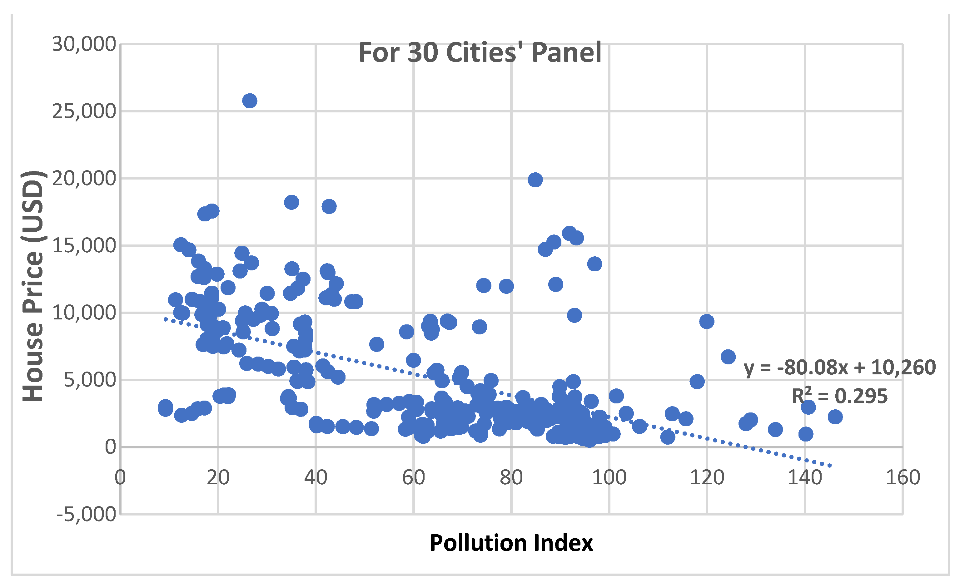
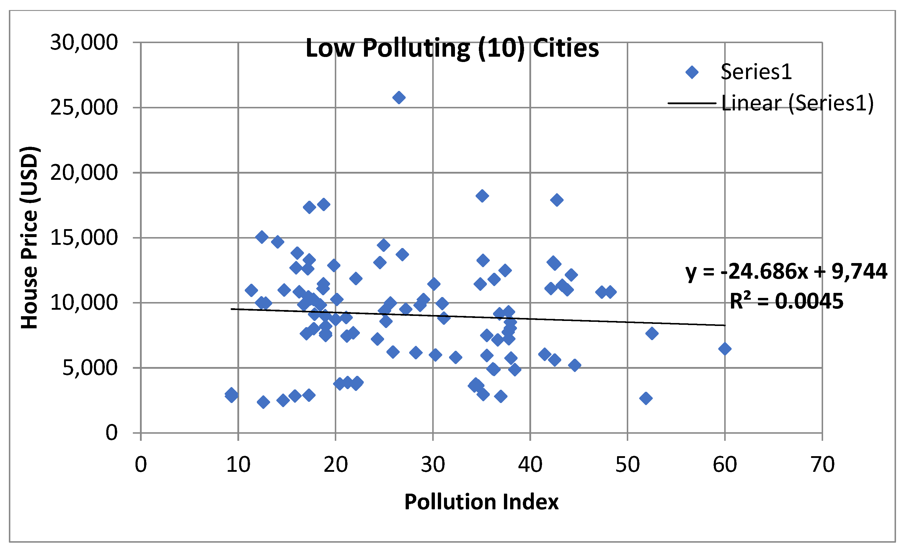
5.1. Graphical Views

The graphical view of the two datasets for the three different panels is presented in scatter diagrams in Figure 2, Figure 3 and Figure 4, respectively, for the total panel of 30 cities, 20 cities with high pollution, and 10 cities with low pollution, to obtain the trend of the behaviors of the two variables across the cities. Each dot point in the three figures represents the combination of Pollution Index and House Price for each of the countries. The trend lines along all these dot points in the three figures present the trend of the relationship between House Price as dependent variable and Pollution Index as independent variable in the three types of panel data.

Figure 2 shows that there are negative relationships between the pollution levels and house prices in the 30 total cities on average. The trend line shows a negative slope with a magnitude of −80.08, which means that one unit increase in the pollution index of a city leads to a decrease in house prices by USD80, and vice-versa.

Figure 3, for the panel of 20 high-polluting cities, which are mainly cities in developing and less-developed countries, shows an inverse relationship between the two indicators but with a smaller magnitude in the slope of the trend line.

Figure 4, on the other hand, showing the scatter points of the combinations of the two indicators for the 10 low-polluting cities, highlights the same negatively sloped trend line but with relatively higher magnitudes in the slope compared to that of the panel of 20 cities.

This is a clear indication that house price and pollution magnitudes are inversely related, which means that in cities where pollution levels are higher, the house prices will be lower, and vice-versa. This is important empirical evidence as far as the hedonic pricing system in environmental economics is concerned. Under the method of hedonic pricing, the researchers usually estimate the values of environmental services that influence the prices of the marketed goods; areas with good environmental quality are associated with high property values.

5.2. Average Values of the Indicators and Their Degrees of Associations

The essential values of the two indicators are captured by their average (or mean) values.

Table 1. Means and correlation coefficients. Source: Authors’ calculations.

	Mean for All Countries (30)		Mean for Highly Polluting (20)		Mean for Very Low Polluting (10)
	Pollution Index	House Price (USD)	Pollution Index	House Price(USD)	Pollution Index	House Price(USD)
	64	5134	82.08	3172	27.84	9056
Correlation Coefficient (t values)	−0.54 (−11.16)		−0.025 (−0.435)		−0.067 (−1.16)

depicts that the average or mean value of the pollution index is 82.08 for the panel of 20 highly polluting cities, 27.84 for the panel of 10 very-low-polluting cities, and 64 for the whole panel of 30 polluting cities. Conversely, the average values of the housing prices are USD 3172 for the panel of 20 highly polluting cities, USD 9056 for the panel of 10 very-low-polluting cities, and USD 5134 for the whole panel of 30 polluting cities in the world. There is an inverse relationship between the average values of the two indicators across all the panels of the cities.

The study has thus computed the values of the correlation coefficients for all three panels to determine the degree of association between pollution and house prices in these cities. The results from Table 1 show that there are negative correlations between the two for all the three panels of the cities, but the said magnitude is higher for the whole panel, with a value of −0.54. The statistical significance test of this correlation, in line with the ‘t’ test, shows that the said correlation is highly significant, which means that low pollution is associated with high property prices and vice-versa. The other two panels do not produce significant correlations between the two variables. However, correlation does not mean causation; further time-series econometric exercises are required.

5.3. Results of Panel Unit Root Test

Before attempting to investigate whether two variables have long-term associations or short-term dynamics, it is a precondition that the two series should be stationary or should be free from unit root problems to avoid spurious regression results between the two. Stationarity property refers to no past values having impacts upon the current values of the variables, keeping the series to a nearly constant value, or the fluctuations around a constant value. First of all, we started with the cross-sectional dependency (CD) test proposed by Pesaran [70], and after confirming the absence of CD in the majority of the cases in our panel, we proceeded with first-generation panel unit root tests to investigate the integrating features of the two variables of concern. The CD test results are given in

Table 2. CD test results. Source: Authors’ calculations.

Variable	Breusch-Pagan LM		Pesaran Scaled LM		Pesaran LM
	Test Stat.	Prob.	Test Stat.	Prob.	Test Stat.	Prob.
	1487.100	0.00	04.85693	0.2453	−0.85364	0.3125

.

The tests for stationarity of the two series for the balanced panel data are performed by Levin and Lin (LL Test) [59] and Levin, Lin, and Chu (LLC Test) [60] for the common unit root process term, and by Im, Pesaran, and Shin (IPS Test) [61,62], ADF-Fisher Chi-square, and the PP-Fisher Chi-square of Maddala and Wu [63] for the different unit root process terms across the panel member cities.

The study first opted to test the unit root for the level values of the panels for the two indicators but did not find stationarity features (results are not shown in the table to avoid excessive congestion). It thus opted to test stationarity at the first differences between the two indicators across the three sets of panel data. Table 2 presents the data.

The results given in

Table 3. Panel unit root test results for the pollution index and housing prices at first difference. Source: Authors’ calculations.

Methods	Null Hypotheses	Test Statistics by Intercepts (Prob.) All Countries (30)		Test Statistics by Intercepts (Prob.) Highly Polluting (20)		Test Statistics by Intercepts (Prob.) Very Low Polluting (10)
		Pollution	House Price	Pollution	House Price	Pollution	House Price
LLC	No common unit root	−38.23 (0.00)	−15.64 (0.00)	−34.55 (0.00)	−13.76 (0.00)	−13.4 (0.00)	−7.30 (0.00)
IPS	No individual unit roots	−21.46 (0.00)	−7.93 (0.00)	21.27 (0.00)	−6.7 (0.00)	−7.09 (0.00)	−4.19 (0.00)
MW-ADF-Fisher Chi-square	No individual unit roots	342.86 (0.00)	189.22 (0.00)	254.16 (0.00)	130.15 (0.00)	88.13 (0.00)	58.80 (0.00)
MW-PP-Fisher Chi-square	No individual unit roots	468.76 (0.00)	230.85 (0.00)	352.26 (0.00)	163.12 (0.00)	116.2 (0.00)	67.66 (0.00)

Note: Lag length is automatically selected through the AIC: 0 to 6. An asymptotic Chi-square distribution is used for deriving probabilities under Fisher tests. The remaining tests assume asymptotic normality. The results for low-polluting countries are also stationary at the levels.

show that both the series are stationary in their first differences in all three panels of cities. It thus helps to proceed to investigate the existence of long-term relationships between the magnitudes of pollution and house prices for the said panels of cities.

5.4. Results of Panel Cointegration Test

As mentioned in the methodology section, there are usually three techniques to test cointegration, which are the Pedroni, Kao, and Fisher–Johansen tests.

Table 4. Pedroni’s panel cointegration test. Source: Authors’ calculations.

Hypotheses→/Test Criteria↓	Null Hypothesis: No Cointegration		Statistic (Prob)	Weighted Statistic (Prob)
Having no deterministic trend	Alternative hypothesis: Having common AR coefficients (i.e., within-dimension)	Panel v-Stat	−0.09 (0.53) {−0.44 (0.67)} [0.04 (0.48)]	−0.57 (0.71) {−0.72 (0.76)} [0.09 (0.46)]
		Panel rho-Stat	0.84 (0.80) {2.14 (0.98)} [0.08 (0.53)]	0.97 (0.83) {0.57 (0.71)} [0.93 (0.82)]
		Panel PP-Stat	−1.10 (0.13) 2.44 (0.99)} [1.65 (0.05)] *	−1.02 (0.15) {−1.24 (0.10)} [0.17 (0.57)]
		Panel ADF-Stat	−3.37 (0.00) * {0.60 (0.72)} [−3.26 (0.00)] *	−3.44 (0.00) * {−3.37 (0.00)} * [−1.04 (0.15)]
	Alternative hypothesis: Having individual AR coefficients (i.e., between-dimension)	Group rho-Stat	2.89 (0.99) {2.21 (0.98)} [1.86 (0.96)]	-
		Group PP-Stat	−1.2 (0.10) {−1.59 (0.05)} * [0.11 (0.54)]	-
		Group ADF-Stat	−2.84 (0.00) * {−1.91 (0.02)} * [−2.21 (0.01)] *	-
Having both the deterministic intercept and trend	Alternative hypothesis: Having common AR coefficients (i.e., within-dimension)	Panel v-Stat	−1.02 (0.84) {3.21 (0.00)} * [−1.16 (0.87)]	−2.75 (0.99) {−2.88 (0.99)} [−0.26 (0.60)]
		Panel rho-Stat	1.57 (0.94) {1.16 (0.87)} [0.92 (0.82)]	3.27 (0.99) {2.96 (0.99)} [1.28 (0.89)]
		Panel PP-Stat	−6.49 (0.00) * {−3.01 (0.00)} * [−4.18 (0.00)] *	−6.15 (0.00) * {−4.69 (0.00)} * [−4.25 (0.00)] *
		Panel ADF-Stat	−6.97 (0.00) * {−1.69 (0.04)} * [−4.72 (0.00)] *	−8.46 (0.00) * {−7.19 (0.00)} * [−4.29 (0.00)] *
	Alternative hypothesis: Having individual AR coefficients (i.e., between-dimension)	Group rho-Stat	4.49 (0.98) {3.89 (0.99)} [2.28 (0.98)]	-
		Group PP-Stat	−8.47 (0.00) * {−7.53 (0.00)} * [−4.02 (0.00)] *	-
		Group ADF-Stat	−6.67 (0.00) * {−5.20 (0.00)} * [−4.21 (0.00)] *	-
Having no deterministic intercept and trend	Alternative hypothesis: Having common AR coefficients (i.e., within-dimension)	Panel v-Stat	0.42 (0.33) {−0.12 (0.55)} [0.38 (0.34)]	−1.42 (0.93) {−1.57 (0.94)} [−0.13 (0.55)]
		Panel rho-Stat	−5.80 (0.00) * {−5.91 (0.00)} * [−2.29 (0.00)] *	−5.68 (0.00) * {−4.89 (0.00)} [−2.65 (0.00)] *
		Panel PP-Stat	−8.56 (0.00) * {−7.75 (0.00)} * [−4.70 (0.00)] *	−8.81 (0.00) * {−7.68 (0.00)} * [−3.93 (0.00)] *
		Panel ADF-Stat	−2.99 (0.00) * {2.73 (0.99)} [−2.64 (0.00)] *	−3.39 (0.00) * {−2.81 (0.00)} * [−1.91 (0.02)] *
	Alternative hypothesis: Having individual AR coefficients (i.e., between-dimension)	Group rho-Stat	−0.72 (0.23) * {−0.87 (0.18)} [−0.01 (0.48)]	-
		Group PP-Stat	−8.46 (0.00) * {−7.61 (0.00)} * [−3.88 (0.00)] *	-
		Group ADF-Stat	−3.81 (0.00) * {−2.61 (0.00)} * [−2.96 (0.00)] *	-

Note: The * marks indicate significant cointegration results. Second brackets ({}) contain the results for the high-polluting cities and the third brackets ([ ]) contain the results for the low-polluting cities.

,

Table 5. Kao’s cointegration test. Source: Authors’ calculations.

Null Hypothesis: Having No Cointegration	All Countries (30)	Highly Polluting (20)	Low Polluting (10)
	t-Stat (Prob.)	t-Stat (Prob.)	t-Stat (Prob.)
ADF	−0.99 (0.16)	1.13 (0.12)	−1.40 (0.08)

and

Table 6. Cointegration test under Fisher–Johansen method. Source: Authors’ calculations.

Hypothesized No. of CE(s)	All Countries (30)	Highly Polluting (20)	Low Polluting (10)
	Fisher Stat. (Prob.) (from trace test)	Fisher Stat. (Prob.) (from trace test)	Fisher Stat. (Prob.) (from trace test)
None	361.6 (0.00)	241.0 (0.00)	120.6 (0.00)
At most 1	188.6 (0.00)	113.2 (0.00)	78.46 (0.00)

present the respective test results. Each of the tables presents the results for all three panels of cities.

The Pedroni test is run with three diverse classifications—‘having no deterministic trend’, ‘having both the deterministic trend and intercept’, and ‘having no deterministic trend and intercept’. Further, each test classification has two more sub-classifications, ‘within dimensions’ and ‘between dimensions’. There are so many data on the results of the test for the three panels. In most of the cases, the study finds significant cointegrations between pollution and house price in all three panels in two categories—‘with deterministic trends and intercepts’ and ‘no deterministic trend and intercept’. Hence, considering the majority of the results under the Pedroni test, it is concluded that pollution and house prices have long-term or equilibrium relationships in all three panels of the cities. ‘High pollution and low house price’ and ‘low pollution and high house price’ have co-movements in the long term.

The Kao test results as depicted in Table 5 display no significant cointegration between pollution and house prices in all three different panels of cities. The probabilities of the t-test results are well above 0.05, which confirms the null hypothesis of ‘no cointegration’.

The final test of cointegration, that is the Fisher–Johansen test, shows that the trace statistics for all three panels of cities are significantly larger, with very low probability values. In all panels, at most, only one instance of cointegrating equations is found (refer to Table 6).

Combining the results of the three tests of cointegration, the study considers the majority of the results, which show that out of the three, two test techniques (Pedroni and Fisher–Johansen) establish long-term significant associations between the magnitudes of pollution and house prices in all three panels of cities. It thus can be concluded that house prices and pollution intensity in the selected cities are cointegrated as far as the majority of the tests for cointegration are concerned. In other words, house prices and pollution intensity have co-movements in the selected cities in the panel data analysis.

5.5. VECM Test Results

The presence of cointegration among the variables is a long-term singularity, as the past values of the variables relate all the current values to a particular cointegrating equation. However, this does not mean that there should not be any sort of deviation around the equilibrium relation. The magnitudes of these deviations are captured by the error-correction mechanism. In the panel data analysis, the study develops the VECM incorporating optimum lag values of the variables in the existing three panels. The VECM has the automatic capacity to choose the endogenous variable with the exogenous variable/s with the optimum lag. The VECM results not only demonstrate the error correction mechanism around the long-term relationship, but also exhibit the direction of the long-term causal relationships. The results are revealed in

Table 7. VECM results. Source: Authors’ calculations.

Dependent Variables	EC Terms (Prob.)			Whether Errors Corrected			Remarks
	Total (30)	High Polluting (20)	Low Polluting (10)	Total (30)	High Polluting (20)	Low Polluting (10)
D(Pollution)	−0.054 (0.03)	−0.48 (0.00)	0.002 (0.00)	Yes	Yes	No	Long run causality from House Price to Pollution for Total Panel and the panel of high polluting cities but not for the low polluting cities
D(House Price)	86.32 (0.00)	−0.002 (0.00)	−1.25 (0.00)	No	Yes	Yes	Long run causality from Pollution to House Price for the panels of high polluting and low polluting cities but not for the Total Panel

Note: Optimum lag for Total (30), Panel of high-polluting cities and panel of low-polluting cities are derived as 2, 4, and 3, respectively.

.

Results from the VECM show that there are deviations from the long-term relations when pollution becomes the endogenous regressand (or the dependent variable) and house prices are the endogenous regressor (or the independent variable), and the errors or deviations are corrected significantly for the total panel, as well as for the panel of high-polluting cities. The terms capturing the error corrections are found to be negative and statistically significant. This further indicates that all past values of house prices have a long-term causal influence on the magnitude of pollution in these two panels of cities. In other words, the relatively low house prices in the total panel and the panel of high-polluting cities, being the demand side factor, encourage people from these relatively low-income cities to pollute the environment more. The factors behind such an attitude may be the low awareness of environmental quality, fast-growing economic outputs, etc., in the high-polluting cities, which are synchronous to the increasing portion of the inverted U-shaped Kuznets Curve. However, the errors are not corrected, and having no such long-term causality from house prices to pollution for the panel of low-polluting cities may be due to the reverse causes of the panel of high-polluting cities.

On the other hand, when house prices are considered as the endogenous dependent variable, the errors are corrected for the panels of high-polluting and low-polluting cities, causing the error in the short term to be temporary. It also means that the magnitudes of pollution in these two groups of cities have a long-term causal influence on house prices. It is a common phenomenon that high pollution causes low housing prices and low pollution causes high house prices, because good and bad environmental qualities are converted into alternative market prices. Hence, the pollution levels in cities become one of the important determinants of house prices as far as dynamics in long-term relations are concerned. In fact, the long-term bi-lateral causal relations in the panels of high-polluting cities may be due to the fact that some of the cities from so-called developed countries, such as Italy, Spain, etc., have high house prices and high pollution in that panel of cities.

Regarding the panel of cities in which no error correction results are present, there may be other factors responsible for establishing the error correction toward the long-term relationship. The present study cannot attempt to determine such factors.

Beyond this long-term behavior of pollution and house prices, it is possible in the short term that the variables have significant causal interplays. The short-term causality of the Wald Test is capable of exploring this.

Table 8. Short-term causal influence through Wald Test. Source: Authors’ calculations.

Dependent Variables	Chi square (Prob.)			Comments
	Total (30)	High Polluting (20)	Low Polluting (10)
D(Pollution)	6.354 (0.04)	10.16 (0.03)	24.02 (0.00)	House Price → Pollution for all three panels of cities
D(House Price)	25.11 (0.00)	19.17 (0.00)	17.04 (0.00)	Pollution → House Price for all three panels of cities

Note: Optimum lag for Total (30), Panel of high-polluting cities, and panel of low-polluting cities are derived as 2, 4, and 3, respectively.

displays these results.

Having the feature of I(1) series for the pollution index and house prices, the causal interplays are examined with these two first-difference series with optimum lags following the methodology given above. It is interesting to note that there are bilateral causal interplays between the magnitudes of pollution and house prices in all three panels of cities. All the lagged/past values of the corresponding endogenous independent variables have a significant influence on the corresponding endogenous dependent variables. It is thus a reality that high pollution is a cause of low property prices and low pollution is a cause of high property prices. The increasing number of cities in the developing world with rising income and low environmental awareness are, on the other hand, demanding more houses and creating more pollution. The results of the study have some sort of resemblance to a previous study on the impact of low-carbon technology in the construction industry leading to low pollution, as well as causing stakeholders less stress in the workplace [71].

As already shown in the theoretical model of the paper, high pollution in a city increases the cost of living aside from just the pricing of houses or apartments. Citizens have to tolerate pollution and live unhealthy lives. As a result, the relative demand for houses in these highly polluted cities decreases compared to cities with relatively good environmental qualities. The inadequacy of the demand for houses in highly polluted cities keeps house prices low. The reverse arguments are applicable in cities with low pollution indices. The results derived from the presence of long-term associations and short-term dynamic relations between pollution and house prices in the selected cities first support the theoretical model of the paper, as well as the works of researchers mentioned in the above review of the extant literature [30,31,47,48,49].

The world is now at a juncture of the combinations of the effects of both pollution as well as house prices upon their respective counter-dependent variables, house prices and pollution. With the rising awareness of climate change, countries from all income groups are now accepting the challenge to counter the problem of environmental pollution and, accordingly, value the services of the environment through different market prices. High property prices thus should be interlinked with low pollution or a good environment. Once all countries, as well as the United Nations, are capable of valuing all environmental goods and services properly, pollution levels will gradually decrease and the sustainable development goal will be gradually attained. Global policy leaders should frame policies in this direction, putting aside the north–south conflict.

6. Conclusions

6.1. Summary of Results

It is now globally a vibrant topic as to whether housing prices are associated with the quality of the environment in a particular region. The present study started with the objective of investigating whether there are long-term associations and short-term causal interplays between the magnitudes of pollution and house prices in a panel of the world’s highest-polluting and lowest-polluting cities. Using appropriate time-series econometric techniques, the study arrived at the conclusion that the magnitudes of pollution and house prices in cities are cointegrated with a stable long-term relationship in all panels. Further, there are strong causal interplays in the long term, as well as in the short term, from pollution to house prices in most panels of cities.

6.2. Policy Recommendations

The results of long-term stable relations between pollution and house prices, and the causal interplays from the former to the latter, demand strong policy interventions from governments. As there is an inverse relationship between house prices and the magnitude of pollution at the city level, two kinds of intervention are possible. First, citizens may be offered incentives to keep their city clean, and second, policymakers should make proper valuations of environmental services to control pollution at the city level, as well as at the global level. The cleanliness of cities should thus be the top priority of the governments of countries. In addition, the organizational antecedents in terms of reforms in the structures, culture, etc., can be implemented to maintain environmental sustainability in particular [72].

6.3. Limitations of the Study

In this study, we were only able to incorporate 30 cities across the world to explore the nexus between total pollution and housing prices. Moreover, the impacts of specific types of pollution on housing prices have not been included in the present study. Again, a time-series, city-level analysis for the same dataset can also be considered, subject to the accessibility of data. Therefore, the investigation (both in terms of panel and time series) of the said nexus between housing prices and several types of pollution in the presence of pollution with a higher number of cities can be encompassed in the future research plan.

References

1. Intergovernmental Panel on Climate Change (IPCC). Climate Change 2014: Synthesis Report Summary for Policymakers. 2014. Available online: https://www.ipcc.ch/site/a-ssets/uploads/2018/06/-AR5_SYR_FINAL_SPM.pdf (accessed on 3 July 2022).
2. Dogan, E.; Seker, F. Determinants of CO2 emissions in the European Union: The role of renewable and non-renewable energy. Renew. Energy 2016, 94, 429–439. [Google Scholar] [CrossRef]
3. Brunekreef, B.; Holgate, S.T. Air pollution and health. Lancet 2002, 360, 1233–1242. [Google Scholar] [CrossRef]
4. Heyes, A.; Zhu, M. Air pollution as a cause of sleeplessness: Social media evidence from a panel of Chinese cities. J. Environ. Econ. Manag. 2019, 98, 102247. [Google Scholar] [CrossRef]
5. Zhang, H.; Chen, J.; Wang, Z. Spatial heterogeneity in spillover effect of air pollution on housing prices: Evidence from China. Cities 2021, 113, 103145. [Google Scholar] [CrossRef]
6. Alam, S.; Fatima, A.; Butt, M.S. Sustainable development in Pakistan in the context of energy consumption demand and environmental degradation. J. Asian Econ. 2007, 18, 825–837. [Google Scholar] [CrossRef]
7. Al-Mulali, U.; Ozturk, I.; Lean, H.H. The influence of economic growth, urbanization, trade openness, financial development, and renewable energy on pollution in Europe. Nat. Hazards 2015, 79, 621–644. [Google Scholar] [CrossRef]
8. Zafar, M.W.; Zaidi, S.A.H.; Sinha, A.; Gedikli, A.; Hou, F. The role of stock market and banking sector development, and renewable energy consumption in carbon emissions: Insights from G-7 and N-11 countries. Resour. Policy 2019, 62, 427–436. [Google Scholar] [CrossRef]
9. Anwar, A.; Siddique, M.; Dogan, E.; Sharif, A. The moderating role of renewable and non-renewable energy in environment-income nexus for ASEAN countries: Evidence from Method of Moments Quantile Regression. Renew. Energy 2021, 164, 956–967. [Google Scholar] [CrossRef]
10. Pao, H.T.; Tsai, C.M. Multivariate Granger causality between CO2 emissions, energy consumption, FDI (foreign direct investment) and GDP (gross domestic product): Evidence from a panel of BRIC (Brazil, Russian Federation, India, and China) countries. Energy 2011, 36, 685–693. [Google Scholar] [CrossRef]
11. Baek, J. Do nuclear and renewable energy improve the environment? Empirical evidence from the United States. Ecol. Indic. 2016, 66, 352–356. [Google Scholar] [CrossRef]
12. Bakhsh, K.; Rose, S.; Ali, M.F.; Ahmad, N.; Shahbaz, M. Economic growth, CO2 emissions, renewable waste and FDI relation in Pakistan: New evidences from 3SLS. J. Environ. Manag. 2017, 196, 627–632. [Google Scholar] [CrossRef] [PubMed]
13. Hanif, I. Impact of economic growth, nonrenewable and renewable energy consumption, and urbanization on carbon emissions in Sub-Saharan Africa. Environ. Sci. Pollut. Res. 2018, 25, 15057–15067. [Google Scholar] [CrossRef] [PubMed]
14. Koengkan, M. The decline of environmental degradation by renewable energy consumption in the MERCOSUR countries: An approach with ARDL modeling. Environ. Syst. Decis. 2018, 38, 415–425. [Google Scholar] [CrossRef]
15. Hu, H.; Jin, Q.; Kavan, P. A study of heavy metal pollution in China: Current status, pollution-control policies and countermeasures. Sustainability 2014, 6, 5820–5838. [Google Scholar] [CrossRef] [Green Version]
16. BP. BP Statistical Review of World Energy. 2019. Available online: https://www.bp.com/en/global/corporate/energy-economics/statistical-review-of-worldenergy.html (accessed on 2 July 2022).
17. International Energy Agency. Global Energy & CO2 Status Report 2018. 2019. Available online: https://webstore.iea.org/global-energy-co2-status-report2018 (accessed on 2 July 2022).
18. Grossman, G.M.; Krueger, A.B. Environmental Impacts of a North American Free Trade Agreement; National Bureau of Economic Research: Cambridge, MA, USA, 1991. [Google Scholar]
19. Dogan, E.; Inglesi-Lotz, R. The impact of economic structure to the environmental Kuznets curve (EKC) hypothesis: Evidence from European countries. Environ. Sci. Pollut. Res. 2020, 27, 12717–12724. [Google Scholar] [CrossRef]
20. Halicioglu, F. An econometric study of CO2 emissions, energy consumption, income and foreign trade in Turkey. Energy Policy 2009, 37, 1156–1164. [Google Scholar] [CrossRef] [Green Version]
21. Andati, P.; Majiwa, E.; Ngigi, M.; Mbeche, R.; Ateka, J. Determinants of Adoption of Climate Smart Agricultural Technologies among Potato Farmers in Kenya: Does entrepreneurial orientation play a role? Sustain. Technol. Entrep. 2022, 1, 100017. [Google Scholar] [CrossRef]
22. Shahbaz, M.; Tiwari, A.K.; Nasir, M. The effects of financial development, economic growth, coal consumption and trade openness on CO2 emissions in South Africa. Energy Policy 2013, 61, 1452–1459. [Google Scholar] [CrossRef] [Green Version]
23. Katircioglu, S.T. Testing the tourism-induced EKC hypothesis: The case of Singapore. Econ. Model 2014, 41, 383–391. [Google Scholar] [CrossRef]
24. Apergis, N.; Ozturk, I. Testing environmental Kuznets curve hypothesis in Asian countries. Ecol. Indic. 2015, 52, 16–22. [Google Scholar] [CrossRef]
25. Uzar, U.; Eyuboglu, K. The nexus between income inequality and CO2 emissions in Turkey. J. Clean. Prod. 2019, 227, 149–157. [Google Scholar] [CrossRef]
26. Uzar, U.; Eyuboglu, K. Do natural resources heal the environment? Empirical evidence from Turkey. Air Qual. Atmos. Health 2021, 14, 37–46. [Google Scholar] [CrossRef]
27. Eyuboglu, K.; Uzar, U. A new perspective to environmental degradation: The linkages between higher education and CO2 emissions. Environ. Sci. Pollut. Res. 2021, 28, 482–493. [Google Scholar] [CrossRef]
28. Miah, M.D.; Masum, M.F.H.; Koike, M.; Akhter, S.; Muhammed, N. Environmental Kuznets curve: The case of Bangladesh for waste emission and suspended particulate matter. Environmentalist 2011, 31, 59–66. [Google Scholar] [CrossRef]
29. Zhang, X.; Zhang, X.; Chen, X. Happiness in the air: How does a dirty sky affect mental health and subjective well-being? J. Environ. Econ. Manag. 2017, 85, 81–94. [Google Scholar] [CrossRef] [PubMed]
30. Das, R.C.; Ivaldi, E. Is Pollution a Cost to Health? Theoretical and Empirical Inquiry for the World’s Leading Polluting Economies. Int. J. Environ. Res. Public Health 2021, 18, 6624. [Google Scholar] [CrossRef]
31. Chay, K.Y.; Greenstone, M. Does air quality matter? Evidence from the housing market. J. Political Econ. 2005, 113, 376–424. [Google Scholar] [CrossRef] [Green Version]
32. Arya, S.P. Air Pollution Meteorology and Dispersion; Oxford University Press: New York, NY, USA, 1999. [Google Scholar]
33. Seigneur, C. Air Pollution: Concepts, Theory, and Applications; Cambridge University Press: Cambridge, UK, 2019. [Google Scholar]
34. Chen, X.; Ye, J. When the wind blows: Spatial spillover effects of urban air pollution in China. J. Environ. Plan. Manag. 2019, 62, 1359–1376. [Google Scholar] [CrossRef]
35. Lai, Z.; Liu, X.; Li, W.; Li, Y.; Zou, G.; Tu, M. Exploring the Spatial Heterogeneity of Residents’ Marginal Willingness to Pay for Clean Air in Shanghai. Front. Public Health 2021, 9, 791575. [Google Scholar] [CrossRef]
36. Bayer, P.; Keohane, N.; Timmins, C. Migration and hedonic valuation: The case of air quality. J. Environ. Econ. Manag. 2009, 58, 1–14. [Google Scholar] [CrossRef] [Green Version]
37. Zhao, D.; Sing, T.F. Air pollution, economic spillovers, and urban growth in China. Ann. Reg. Sci. 2017, 58, 321–340. [Google Scholar] [CrossRef]
38. Zheng, S.; Kahn, M.E.; Sun, W.; Luo, D. Incentives for China’s urban mayors to mitigate pollution externalities: The role of the central government and public environmentalism. Reg. Sci. Urban Econ. 2014, 47, 61–71. [Google Scholar] [CrossRef]
39. Cui, X.; Fang, C.; Liu, H.; Liu, X. Assessing sustainability of urbanization by a coordinated development index for an Urbanization-Resources-Environment complex system: A case study of Jing-Jin-Ji region, China. Ecol. Indic. 2019, 96, 383–391. [Google Scholar] [CrossRef]
40. Yu, Y.; Zhang, N.; Kim, J.D. Impact of urbanization on energy demand: An empirical study of the Yangtze River Economic Belt in China. Energy Policy 2020, 139, 111354. [Google Scholar] [CrossRef]
41. Das, R.C.; Chatterjee, T.; Ivaldi, E. Sustainability of Urbanization, Non-Agricultural Output and Air Pollution in the World’s Top 20 Polluting Countries. Data 2021, 6, 65. [Google Scholar] [CrossRef]
42. Xiaoyang, L.; Lu, Z.; Hou, Y.; Zhao, G.; Zhang, L. The coupling coordination degree between urbanization and air environment in the Beijing(Jing)-Tianjin(Jin)-Hebei(Ji) urban agglomeration. Ecol. Indic. 2022, 137, 108–787. [Google Scholar]
43. Xie, Y.; Dai, H.; Dong, H.; Hanaoka, T.; Masui, T. Economic impacts from PM 2.5 pollution-related health effects in China: A provincial-level analysis. Environ. Sci. Technol. 2016, 50, 4836–4843. [Google Scholar] [CrossRef]
44. Zheng, S.; Kahn, M.E. Understanding China’s urban pollution dynamics. J. Econ. Lit. 2013, 51, 731–772. [Google Scholar] [CrossRef] [Green Version]
45. Zou, Y.H. Air pollution and housing prices across Chinese cities. J. Urban Plan. Dev. 2019, 145, 04019012. [Google Scholar] [CrossRef]
46. Conceiçao, P. Beyond Income, beyond Averages, beyond Today: Inequalities in Human Development in the 21st Century; United Nations Development Programme (UNDP): New York, NY, USA, 2019. [Google Scholar]
47. United Nations Economic and Social Commission for Asia and the Pacific (UNESCAP). Report—Fourth South Asia Forum on the Sustainable Development Goals; UNESCAP: Bangkok, Thailand, 2021; Available online: https://www.unescap.org/kp/2021/report-fourth-south-asia-forum-sustainable-development-goals (accessed on 5 June 2022).
48. Chopra, M.; Singh, S.K.; Gupta, A.; Aggarwal, K.; Gupta, B.B.; Colace, F. Analysis & prognosis of sustainable development goals using big data-based approach during COVID-19 pandemic. Sustain. Technol. Entrep. 2022, 1, 100012. [Google Scholar] [CrossRef]
49. Jacobson, M.Z. Atmospheric Pollution: History, Science, and Regulation; Cambridge University Press: New York, NY, USA, 2002. [Google Scholar]
50. Smith, V.K.; Huang, J.C. Can markets value air-quality—A meta analysis of hedonic property value models. J. Political Econ. 1995, 103, 209–227. [Google Scholar] [CrossRef]
51. Zabel, J.E.; Kiel, K.A. Estimating the demand for air quality in four US cities. Land Econ. 2000, 76, 174–194. [Google Scholar] [CrossRef]
52. Yusuf, A.A.; Resosudarmo, B.P. Does clean air matter in developing countries’ megacities? A hedonic price analysis of the Jakarta housing market, Indonesia. Ecol. Econ. 2009, 68, 1398–1407. [Google Scholar] [CrossRef]
53. Chen, J.; Hao, Q.; Yoon, C. Measuring the welfare cost of air pollution in Shanghai: Evidence from the housing market. J. Environ. Plan Manag. 2018, 61, 1744–1757. [Google Scholar] [CrossRef]
54. Carriazo, F.; Gomez-Mahecha, J.A. The demand for air quality: Evidence from the housing market in Bogota, Colombia. Environ. Dev. Econ. 2018, 23, 121–138. [Google Scholar] [CrossRef] [Green Version]
55. Chen, S.Y.; Jin, H. Pricing for the clean air: Evidence from Chinese housing market. J. Clean. Prod. 2019, 206, 297–306. [Google Scholar] [CrossRef]
56. Dong, J.; Zeng, X.; Mou, X.; Li, X. Pay for clean air or not? The impact of air quality on China’s real estate price. Syst. Eng. Theor. Pract. 2020, 40, 1613–1626. [Google Scholar] [CrossRef]
57. Le Boennec, R.; Salladarre, F. The impact of air pollution and noise on the real estate market. The case of the 2013 European Green Capital: Nantes, France. Ecol. Econ. 2017, 138, 82–89. [Google Scholar] [CrossRef] [Green Version]
58. Kaklauskas, A.; Zavadskas, E.K.; Radzeviciene, A.; Ubarte, I.; Podviezko, A.; Podvezko, V.; Kuzminsk, A.; Banaitis, A.; Binkyte, A.; Bucinskas, V. Quality of city life multiple criteria analysis. Cities 2018, 72, 82–93. [Google Scholar] [CrossRef]
59. Levin, A.; Lin, C.F. Unit Root Tests in Panel Data: New Results; Discussion Paper; University of California: San Diego, CA, USA, 1993. [Google Scholar]
60. Levin, A.; Lin, C.F.; Chu, C.S.J. Unit root tests in panel data: Asymptotic and finite-sample properties. J. Econom. 2002, 108, 1–24. [Google Scholar] [CrossRef]
61. Im, K.S.; Pesaran, M.H.; Shin, Y. Testing for Unit Roots in Heterogeneous Panels. Cambridge Working Papers in Economics, Cambridge, UK. Mimeo 1997. Available online: https://econpapers.repec.org/RePEc:cam:camdae:9526 (accessed on 5 June 2022).
62. Im, K.S.; Pesaran, M.H.; Shin, Y. Testing for Unit Roots in Heterogeneous Panels. J. Econom. 2003, 115, 53–74. [Google Scholar] [CrossRef]
63. Maddala, G.S.; Wu, S. A Comparative Study of Unit Root Tests with Panel Data and A New Simple Test. Oxf. Bull. Econ. Stat. 1999, 61, 631–652. [Google Scholar] [CrossRef]
64. Pedroni, P. Critical Values for Cointegration Tests in Heterogeneous Panels with Multiple Regressors. Oxf. Bull. Econ. Stat. 1999, 61, 653–670. [Google Scholar] [CrossRef]
65. Pedroni, P. Panel Cointegration: Asymptotic and Finite Sample Properties of Pooled Time Series Tests with an Application to the PPP Hypothesis. Econom. Theory 2004, 20, 597–625. [Google Scholar] [CrossRef] [Green Version]
66. Kao, C. Spurious Regression and Residual-Based Tests for Cointegration in Panel Data. J. Econom. 1999, 90, 1–44. [Google Scholar] [CrossRef]
67. Engle, R.F.; Granger, C.W. Co-integration and error correction: Representation, estimation and testing. Econometrica 1987, 55, 251–276. [Google Scholar] [CrossRef]
68. Johansen, S. Statistical analysis of cointegration vectors. J. Econ. Control. 1988, 12, 231–254. [Google Scholar] [CrossRef]
69. Fisher, R.A. Statistical Methods for Research Workers; Oliver and Boyd: Edinburgh, UK, 1932. [Google Scholar] [CrossRef]
70. Pesaran, M.H. A simple panel unit root test in the presence of cross-section dependence. J. Appl. Econom. 2007, 22, 265–312. [Google Scholar] [CrossRef] [Green Version]
71. Esmaeilifar, R.; Iranmanesh, M.; Shafiei, M.W.M.; Hyun, S.S. Effects of low carbon waste practices on job satisfaction of site managers through job stress. Rev. Manag. Sci. 2020, 14, 115–136. [Google Scholar] [CrossRef]
72. Tipu, S.A.A. Organizational change for environmental, social, and financial sustainability: A systematic literature review. Rev. Manag. Sci. 2021, 16, 1697–1742. [Google Scholar] [CrossRef]
Figure 1. Illustration of the mechanism of hedonic pricing.
Sustainability 14 09283 g001
Figure 2. Scatter diagram of pollution index and house price for the total panel. Source: Drawn by the authors.
Sustainability 14 09283 g002
Figure 3. Scatter diagram of pollution index and house price for the panel of high-polluting cities. Source: Drawn by the authors.
Sustainability 14 09283 g003
Figure 4. Scatter diagram of pollution index and house price for the panel of low-polluting cities. Drawn by the authors.
Sustainability 14 09283 g004