Spatiotemporal Complementary Characteristics of Large-Scale Wind Power, Photovoltaic Power, and Hydropower

Abstract

With the increasing proportion of renewable energy in power generation, the mixed utilization of multiple renewable energy sources has gradually become a new trend. Using the natural complementary characteristics of wind power, photovoltaic, and hydropower to evaluate the complementary potential of various energy sources has become a hot issue in the research of mixed utilization. Given that traditional complementarity research can only assess the complementarity between two energy sources, this paper proposes a method to simultaneously determine the complementarity between three large-scale renewable energy sources. Firstly, a three-dimensional vector represents the complementary characteristic combination of any two energy sources. The complementary characteristics of the three energy sources were obtained by finding the optimal solution for the three-dimensional vector. Finally, power stations were selected, located in different spatial areas on the world’s largest renewable energy base in Qinghai, China, as the research object to analyze and verify the complementary characteristics of wind-power–photovoltaic-power–hydropower at different spatiotemporal scales. The results show significant differences in the complementary characteristics of different time scales. The farther the spatial distance between different power stations, the stronger their complementarity. The best complementary index on the monthly and daily scales was improved by 8.49% and 6.51%. This study provides a new focus for the future evaluation of the complementary utilization potential of large-scale joint renewable energy in different world regions.

1. Introduction

With the large consumption of non-renewable resources, such as coal, oil, and natural gas, and increasingly severe environmental pollution problems, it is more serious and urgent to replace traditional energy with renewable energy, such as hydropower, solar power, and wind energy [1,2]. However, renewable energy, represented by photovoltaic and wind power, has intermittency, volatility, and randomness in the regeneration process. As a result, after large-scale renewable energy is centrally connected to the power system, it seriously impacts the power quality and operation stability of the main power grid. This results in problems such as wind abandonment, light abandonment, and even disconnection [3], which will turn renewable energy into ‘garbage power’ that is not conducive to grid connection, to a certain extent. In this case, it is a new idea to improve renewable energy’s utilization rate by integrating and coordinating hydropower with photovoltaic and wind power to form a complementary relationship [4].

However, due to geographical location, weather conditions, installed capacity, and other factors, it is not simple to integrate solar energy, hydropower, and wind energy into a traditional power system for stable operation [5]. The power generation scale and utilization time may vary greatly every month, every day, or even every hour, which requires the system operator to have good flexibility to realize the safe and efficient utilization of new energy power generation. Analyzing different energy complementarities can effectively help system operators achieve this goal. According to the background and objectives of power system design and research, researchers usually use mathematical and statistical analysis, such as Pearson correlation coefficient [6], Spearman’s correlation coefficient [7], Kendall correlation coefficient [8], graphical analysis [9], and other methods, to reflect the strength of complementarity through the analysis of correlation, and present the possibility of the complementary utilization of various renewable energies from the perspective of mathematical analysis. It has been proved that the multi-energy complementary comprehensive utilization performance is somewhat optimal.

Presently, countries worldwide have launched research on the complementarity of multiple energy sources. For example, Moura [10] analyzed Portugal’s wind, photovoltaic, and hydropower complementarity. Rosa [11] analyzed and evaluated the complementary potential of small hydropower stations, wind farms, and PV in Rio de Janeiro, Brazil. François [12] studied the complementarity between small hydropower stations and photovoltaic power generation in Italy, but its tedious calculation is not suitable for large-scale renewable energy system applications. Ma [13] analyzed the output characteristics of the Hong Kong wind–solar complementary system from a time domain perspective. Still, it did not establish a reasonable index to measure the intensity of complementarity. Considering the uncertainty of the operation cost of a power system and natural gas system, He [14] proposed a full-day-ahead scheduling model for optimal and coordinated operation of the integrated energy system, but there was no long-term optimal operation research. Philip [15] used reanalysis data to study the daily changes in wind energy and solar radiation in the UK and their impact on the balance of renewable energy supply. Priscilla [16] conducted trend fluctuation analysis and trend correlation analysis on the correlation and cross-correlation. Dirk [17] assessed the complementarity of 33 European countries’ wind resources from 1971–2010 by identifying the time scales explaining the largest variance in the time series of daily wind energy yield. Abhnil [18] provided a systematic quantitative analysis of the Australian continent’s complementary characteristics of solar and wind resources.

At present, relevant research at home and abroad have certain limitations: (1) the research on complementarity mainly focuses on two kinds of energy, and lacks the description of the overall complementary characteristics among three or more types of energy; (2) the analysis mainly focuses on small-scale hydropower stations, and small-scale photovoltaic and wind power, and lacks research on the complementary characteristics between large-scale renewable energy sources; (3) the existing research mainly focuses on the complementary characteristics of the same spatial region, and lacks the research on the complementary characteristics of renewable energy in different space regions; (4) the current studies mainly focus on the complementary attributes of renewable energy in a single time scale, and lack research on the complementary characteristics of renewable energy in multiple time scales.

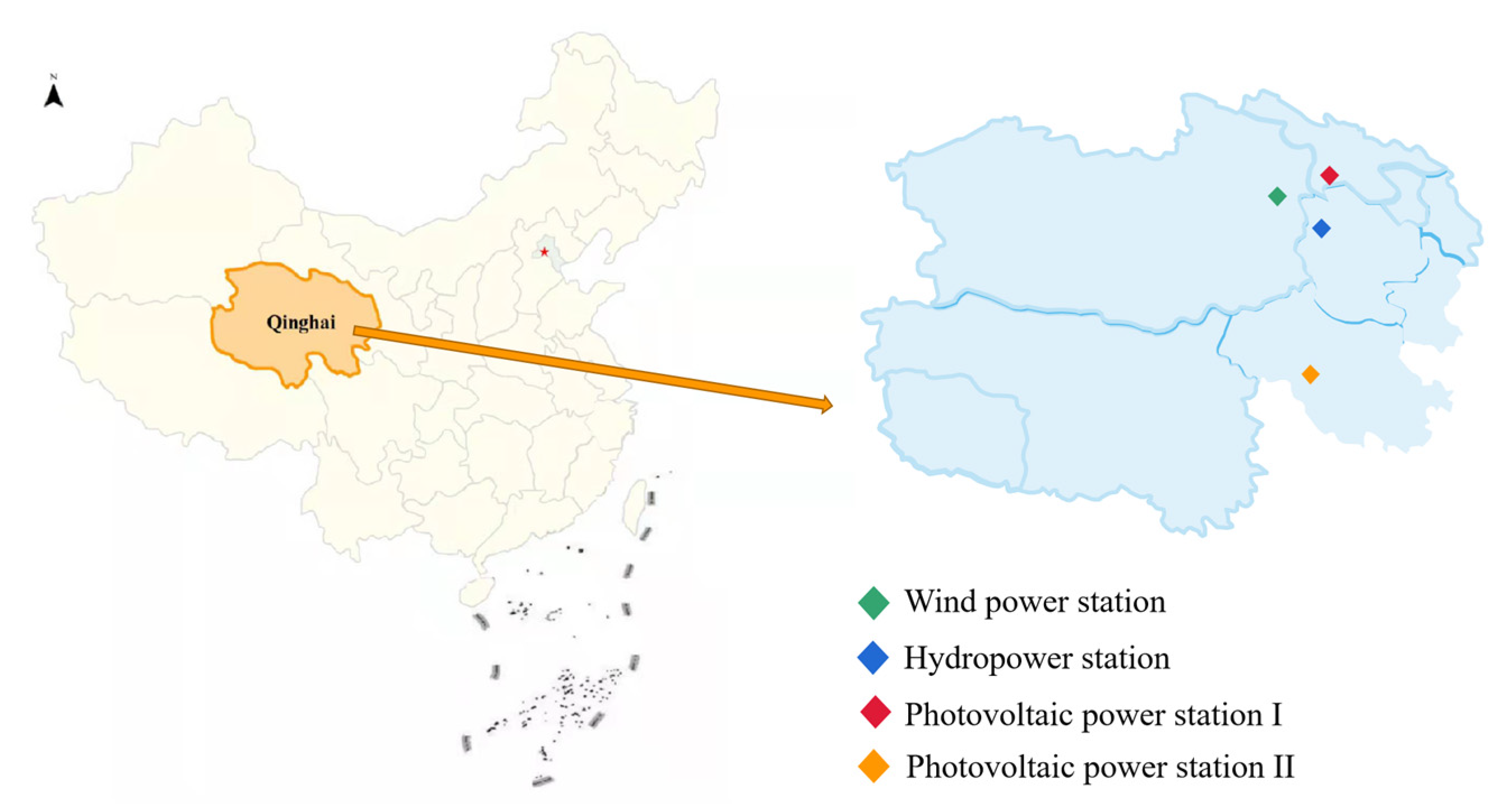
In this context, this paper proposes a new method to simultaneously evaluate the complementarity between the three energy sources using the three-dimensional optimization vector. The spatiotemporal complementary characteristics of multi-energy complementarity under different time scales and geographical positions are analyzed and verified, taking the world’s largest renewable energy base—the upper reaches of the Yellow River in Qinghai, China—as the research object. This paper verifies the effectiveness of the proposed model, and provides a new focus for the future evaluation of the potential of the large-scale complementary utilization of renewable energy.

The research structure of this paper is as follows: the spatiotemporal complementary characteristics of wind power, photovoltaic power, and hydropower and a multidimensional complementary index based on a space vector are described in Section 2. Section 3 probes into a case study, and Section 4 examines its results. Finally, the conclusions of the study are drawn in Section 5.

2. Method

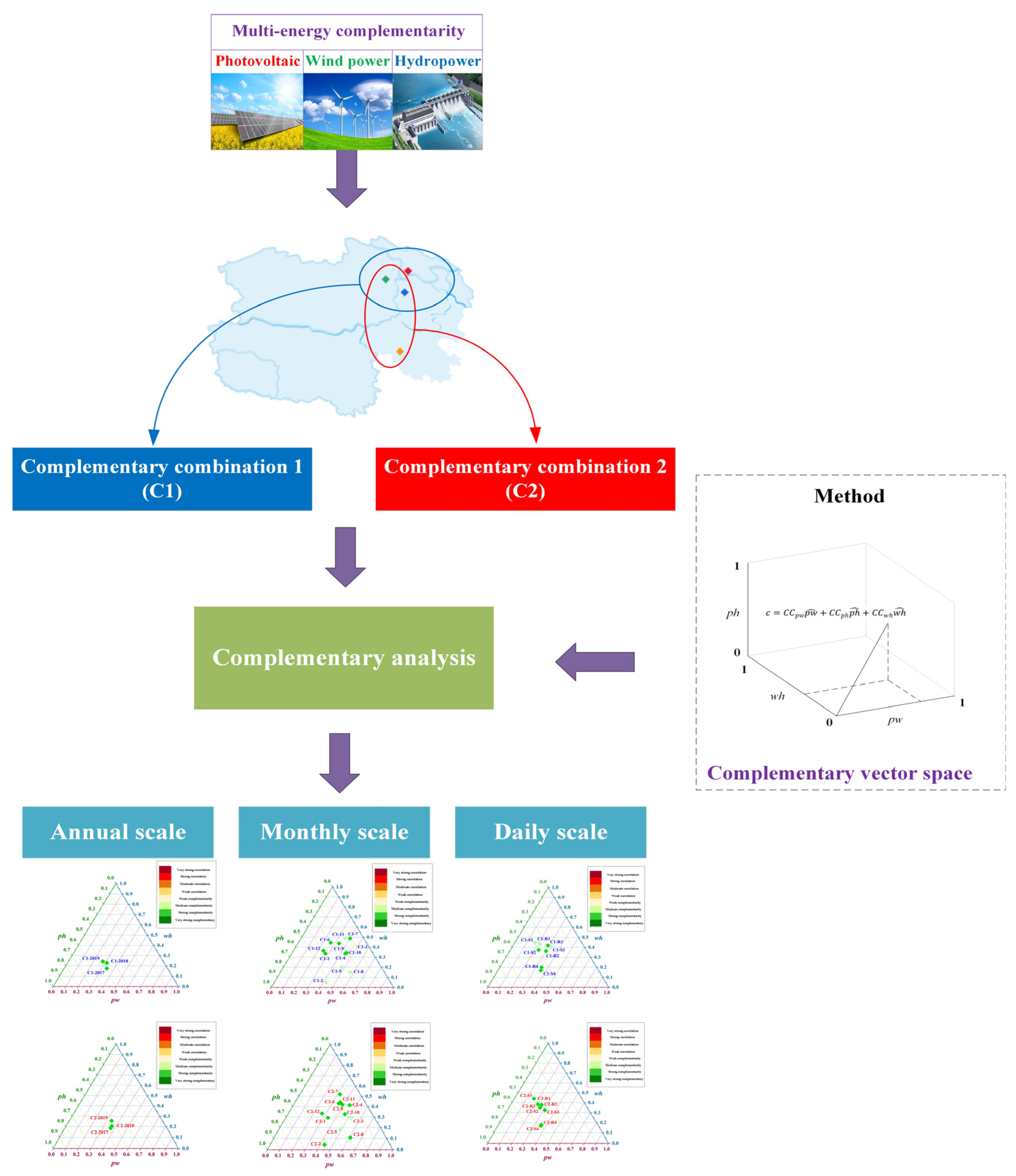
According to the space-time distribution characteristics of different energy sources, large-scale wind power, hydropower, and photovoltaic power stations located in different geographical locations are selected as the research objects. Yearly, monthly, and daily scales are chosen to analyze the complementary characteristics. A multidimensional complementary index based on a space vector describes the overall complementary degree of wind power, hydropower, and photovoltaic power. The research structure is shown in Figure 1.

2.1. Complementary Characteristic Analysis Based on the Correlation Coefficient

In the study of renewable energy complementarity, the Pearson correlation coefficient, Spearman’s correlation coefficient, and Kendall correlation coefficient are commonly used to reflect the complementarity of different energy sources. The value of the correlation coefficient is usually within the range (−1, 1). A correlation coefficient close to 0 indicates almost no correlation between the two groups of variables. A positive correlation coefficient indicates that with the increase or decrease of one group of variables, the other group of variables will also increase or decrease, and a negative correlation coefficient indicates that when one group of variables increases, the other group of variables will decrease; when one group of variables decreases, another group of variables increases. This correlation corresponds to the complementarity of different energy sources: in a multi-energy complementary system, when the output of one energy source decreases, the output of the other energy source increases; when the output of one energy source increases, the output of the other energy source decreases. This complementary operation mode will effectively reduce the output fluctuation of the integrated energy system and maintain stability. According to the research of Canales et al. [19],

Table 1. The complementary correlation coefficient values.

	Correlation Coefficient (r)	Meaning
Correlation	0.9 ≤ r ≤ 1.0	Very strong correlation
	0.6 ≤ r < 0.9	Strong correlation
	0.3 ≤ r < 0.6	Moderate correlation
	0.0 ≤ r < 0.3	Weak correlation
Complementarity	−0.3 < r ≤ 0.0	Weak complementarity
	−0.6 < r ≤ −0.3	Medium complementarity
	−0.9 < r ≤ −0.6	Strong complementarity
	−1.0 ≤ r ≤ −0.9	Very strong complementary

Source: Own study based on Canales et al. [19].

gives the corresponding relationship of energy complementary correlation coefficient values.

Since the Pearson correlation coefficient is only valid for data that conform to or are close to the normal distribution, and the output of wind power, photovoltaic, and hydropower does not conform to the normal distribution, the Pearson correlation coefficient cannot be used to reflect the complementary characteristics between different energy sources; Spearman’s correlation coefficient is a nonparametric statistical method that uses the data’s rank for linear correlation analysis. The size of the correlation coefficient only depends on the order of data, and cannot strictly describe the correlation of data according to time series. Based on this, this paper selects the Kendall correlation coefficient to analyze the output of various energy sources in a time series manner.

The Kendall correlation coefficient is a correlation measure based on the rank of random variables, reflecting the monotonic correlation between variables; that is, the consistency of change trend.

Suppose {(x₁, y₁),(x₂, y₂),…,(x_N, y_N)} is a sample space composed of N sets of observations of random vectors (X, Y), where X and Y are continuous random variables, and x_i and y_i are one-to-one in time. (x_i, y_i) and (x_j, y_j) are any two sets of observations in the sample space. If (x_i, y_i)(x_j, y_j) > 0, then (x_i, y_i) and (x_j, y_j) are consistent; if (x_i, y_i)(x_j, y_j) < 0, then (x_i, y_i) and (x_j, y_j) are inconsistent. The Kendall correlation coefficient represents the difference between the consistent and inconsistent probability of two groups of observations randomly selected from the sample. The calculation method is as follows:

$$r_k=\frac{C-D}{\frac{1}{2}N(N-1)}$$

(1)

where C represents the logarithm of coefficient elements in the sample, D represents the logarithm of inconsistent elements in the model, and the range of r_k is (−1, 1).

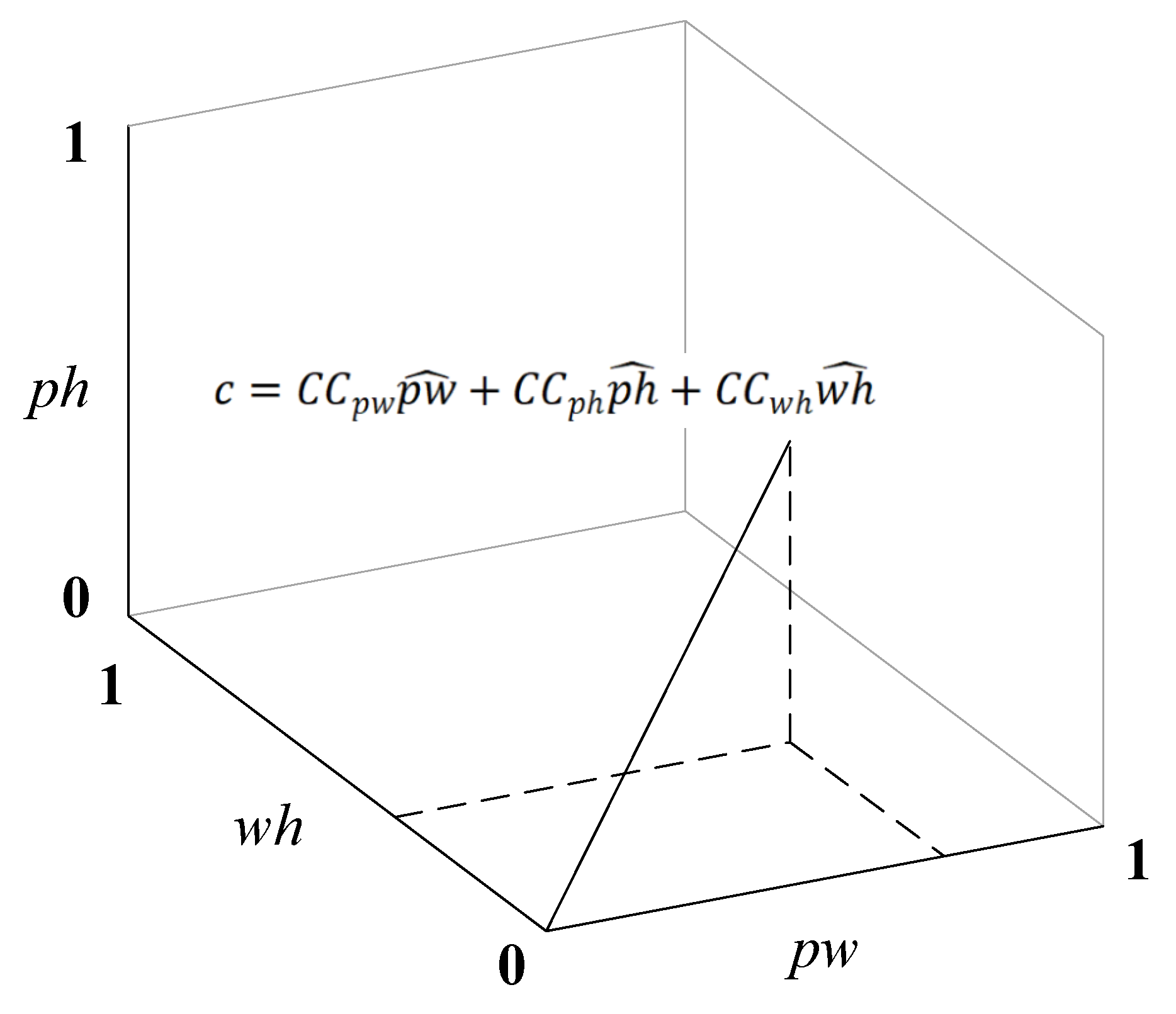
2.2. Multidimensional Complementary Index Based on a Space Vector

A three-dimensional complementary vector, c, is constructed to represent the wind-power–photovoltaic-power–hydropower complementary characteristics. Each correlation coefficient (CC) calculated by the Kendall correlation coefficient is a component of the complementary vector, c. The value of CC represents the complementarity or correlation between each pair of energy sources. The three-dimensional complementary vector, c, is shown in Formula (2):

$$c=C{C}_{pw}\widehat{pw}+C{C}_{ph}\widehat{ph}+C{C}_{wh}\widehat{wh}$$

(2)

where p stands for photovoltaic, w for wind power, h for hydropower, pw denotes the photovoltaic-power–wind-power complementary vector, ph denotes the photovoltaic-power–hydropower complementary vector, and wh denotes the wind-power–hydropower complementary vector. The representation of vector c in three-dimensional space is shown in Figure 2.

The three-dimensional complementary characteristics of energy combination can measure the complementary degree of any group of energy combinations at the same time. However, this three-dimensional vector can only show the degree of complementarity of two energy sources; it cannot analyze the complementary characteristics of three energy sources simultaneously, so it needs further analysis.

In this paper, the compromise programming algorithm is selected to process the three-dimensional vector data further, calculate the distance between each three-dimensional vector solution and the optimal solution, and obtain the overall complementary index of the three energy sources [20]. The distance formula for finding the closest optimal solution in the feasible solution domain of three-dimensional vector space is as follows:

$$L\left(c\right)={\displaystyle \sum }_{k=1}^n{\alpha }_k\left|\frac{f_k^{best}-f_k\left(c\right)}{f_k^{best}-f_k^{worst}}\right|$$

(3)

where ${\alpha }_k$ is the weight of each component, k; and k is each group of complementary energy. The method proposed in this paper holds that each group of complementary energy has the same importance; that is, ${\alpha }_k=1$. $f_k\left(c\right)$ is the CC value of each group of energy combinations corresponding to vector c in Formula (2). $f_k^{best}$ is the optimal function value in three-dimensional vector space, meaning the complete complementarity, so $f_k^{best}=-1. f_k^{worst}$ is the worst function value in the three-dimensional vector space, meaning there is no complementarity, i.e., complete correlation, so $f_k^{worst}=1$.

The wind-power–photovoltaic-power–hydropower total complementary index can be obtained by standardizing the value of $L\left(c\right)$:

$$k_t\left(c\right)=\frac{L{\left(c\right)}_{max}-L\left(c\right)}{L{\left(c\right)}_{max}-L{\left(c\right)}_{min}}$$

(4)

According to Equation (3), the theoretical maximum value of $L\left(c\right)$ is 1, which occurs when the correlation coefficient = 1. The two energy sources are wholly correlated and have the same output curve, which can occur in practice, so the actual maximum value of $L\left(c\right)$ is 1.

The theoretical minimum value of $L\left(c\right)$ is 0, which occurs when the correlation coefficient = −1; that is, the two energy sources are entirely complementary, which cannot happen in practice. Therefore, it is necessary to solve the actual minimum value of $L\left(c\right)$.

The objective function is:

$$MINIMIZE L\left(c\right)={\sum }_{k=1}^n{\alpha }_k\left|\frac{f_k^{best}-f_k\left(c\right)}{f_k^{best}-f_k^{worst}}\right|$$

(5)

setting the objective function $MINIMIZE L\left(c\right)$ to obtain the actual minimum value of $L\left(c\right)$. The $MINIMIZE L\left(c\right)$ could be transformed into finding the minimum value of $f_k\left(c\right).$ $f_k\left(c\right)$ represents the correlation coefficient between different energy sources; that is, the minimum value of the correlation coefficient is solved.

The correlation coefficient problem could be transformed into a purely mathematical calculation problem for analysis to solve it better. In mathematical calculation, the data correlation coefficient is the normalization of covariance, so the solution of the correlation coefficient is transformed into variance calculation. Suppose there are n variables, x_i, and the sum of their variances is:

$$\begin{array}{cc}Var\left({\sum }_{i=1}^n{x}_i\right)& ={\sum }_{i,j=1}^{n}Cov\left(x_i,x_j\right)\hfill \\ & ={\sum }_{i=1}^{n}Var\left(x_i\right)+{\sum }_{i\ne j}Cov\left(x_i,x_j\right)\hfill \\ & =n+{\sum }_{i\ne j}\left({\rho }_{i,j}\times \sqrt{D_{x_i}\times D_{x_j}}\right)\hfill \end{array}$$

(6)

where ${\rho }_{i,j}$ denotes the correlation coefficient of $x_i,x_j$, with a value range of (−1, 1). $D_{x_i},D_{x_j}$ denotes the correlation coefficient of $x_i,x_j$, so $D_{x_i},D_{x_j}=1$. Equation (6) can be converted to:

$$\begin{array}{cc}Var\left({\sum }_{i=1}^n{x}_i\right)& =n+{\sum }_{i\ne j}{\rho }_{i,j}\hfill \\ & =n+\frac{2n!}{2\left(n-2\right)!}\overline{\rho }\hfill \\ & =n+n\left(n-1\right)\overline{\rho }\hfill \end{array}$$

(7)

For any variable, x_i, there is always $D_x\ge 0$; that is, $Var\left({\sum }_{i=1}^n{x}_i\right)\ge 0$. Therefore:

$$\begin{gathered} n+n\left(n-1\right)\overline{\rho }\ge 0 \\ \overline{\rho }\ge -\frac{1}{n-1} \end{gathered}$$

(8)

In our case, n represents the type of energy, so n = 3. Then, $\overline{\rho }\ge -0.5$ is obtained. By substituting the $MINIMIZE L\left(c\right)$ function, we can get $L\left(c\right)\ge$0.75; that is, the actual minimum value of $L\left(c\right)$ is 0.75.

3. Case Study

3.1. Study Area

The built framing is tested by the world’s largest renewable energy resource bases in the upstream area of the Yellow River in China [21]. This area is in the southeast of Qinghai Province, China, and is rich in photovoltaic power, wind power, hydropower, and other renewable energy resources, but the precipitation is deficient. The annual rainfall of Qinghai Province is only 350 mm, mainly in summer [5]. The location of the upstream area of the Yellow River is shown in Figure 3.

To better evaluate spatial distance’s impact on complementary characteristics, this paper selects two photovoltaic power stations more than 500 km apart to study the complementary characteristics at different time scales [22,23]. The data of wind speed, wind force, temperature, and solar radiation in the upstream area of the Yellow River were provided by the China Integrated Meteorological Information Sharing System (CIMISS).

3.2. Power Modeling

(1)

Wind Power Model

The wind power output, P_w, is the power generation of wind turbines under different wind speed conditions, and will be calculated as follows [24]:

$$P_w=\left\{\begin{array}{lll}0& v\le v_i\hspace{1em} or& v\ge v_o\\ P_r\frac{v-v_i}{v_r-v_i}& v_i\le v\le v_r & \\ P_r& v_r\le v\le v_o & \end{array}\right.$$

(9)

where P_r denotes the rated wind output under the rated conditions; v denotes the real-time wind speed; v_i denotes the cut-in wind speed; v_o denotes the cut-out wind speed; v_r denotes the rated wind speed.

(2)

Photovoltaic Model

The photovoltaic output, P_p, is linearly related to the solar light intensity, and is calculated as follows [25]:

$$P_p=P_r\frac{G}{G_r}[1+{\alpha }_T(T-T_r)]$$

(10)

where P_r denotes the rated photovoltaic output under the rated conditions; G denotes the actual solar irradiance (W/m²); G_r denotes the rated solar irradiance (1000 W/m²); α_T denotes the temperature coefficient; T denotes the actual surface temperature of the photovoltaic cells (°C); T_r denotes the rated surface temperature of the photovoltaic cells (25 °C).

(3)

Hydropower Model

This study only deals with reservoir power plants. The high-water period, low-water period, environmental flows (such as meltwater, rainfall, evaporated water, etc.), and tributary flows are all not considered, in order to simplify the calculations in this study. The output power P_h will be calculated as follows [26]:

$$P_h={\eta }_{h}gh\rho Q$$

(11)

where g denotes the gravitational acceleration (9.81 m/s²); η_h denotes the efficiency of the generator; ρ denotes the density of the water (1000 kg/m³); Q denotes the water flow (m³/s); h denotes the height of the water drop (m).

The constraints of wind power, photovoltaic power, and hydropower are as follows [27]:

$$\left\{\begin{array}{l}0\le P_W\le P_{W,max}\\ 0\le P_P\le P_{P,max}\\ V_{t+1}=V_t+(I_t-Q_t)\Delta t\\ V_t^l\le V_t\le V_t^u\\ Q_{tmin}\le Q_t\le Q_{tmax}\\ N_t^l\le N_t\le N_t^u\\ N_s=N_t-N_t^l\end{array}\right.$$

(12)

P_W,max denotes the wind power rated output (MW);

P_P,max denotes the photovoltaic rated output (MW);

V_t+1 and V_t denote the reservoir storage (m³) at the end and the beginning; I_t denotes the reservoir inflow (m³/s);

$V_t^l$ and $V_t^u$ denote the lower and upper limits for reservoir storage (m³);

$Q_t^l$ and $Q_t^u$ denote the lower and upper limits for river discharge flow (m³/s);

$N_t^l$ denotes the lower limits for hydropower output (MW) (the output of the reservoir must be discharged for meeting the downstream irrigation, water supply, navigation, etc.); $N_t^u$ denotes the upper limits for hydropower output (MW);

N_s denotes the schedulable output (MW), which refers to the output that hydropower can offer on the satisfying water-dispatching premise.

4. Results and Discussion

This section sets the installed capacity of the wind power, photovoltaic power, and hydropower as the same: 300 MW. Two photovoltaic power stations more than 500 km apart are selected to better evaluate spatial distance’s impact on the complementary characteristics. The multi-energy complementary combination is divided into C1 (wind power, hydropower, and photovoltaic I) and C2 (wind power, hydropower, and photovoltaic II) groups. This paper selects three time scales, yearly, monthly, and daily, to analyze the complementary characteristics.

The power generation data of wind power, photovoltaic power, and hydropower at three time scales (yearly, monthly, and daily) are substituted into Formula (2) to obtain three-dimensional vector sets at different time scales. Using Formulas (3) and (4), the optimal solution, $k_t\left(c\right)$, of the three-dimensional space vector set is obtained, representing the optimal complementary index under different time scales.

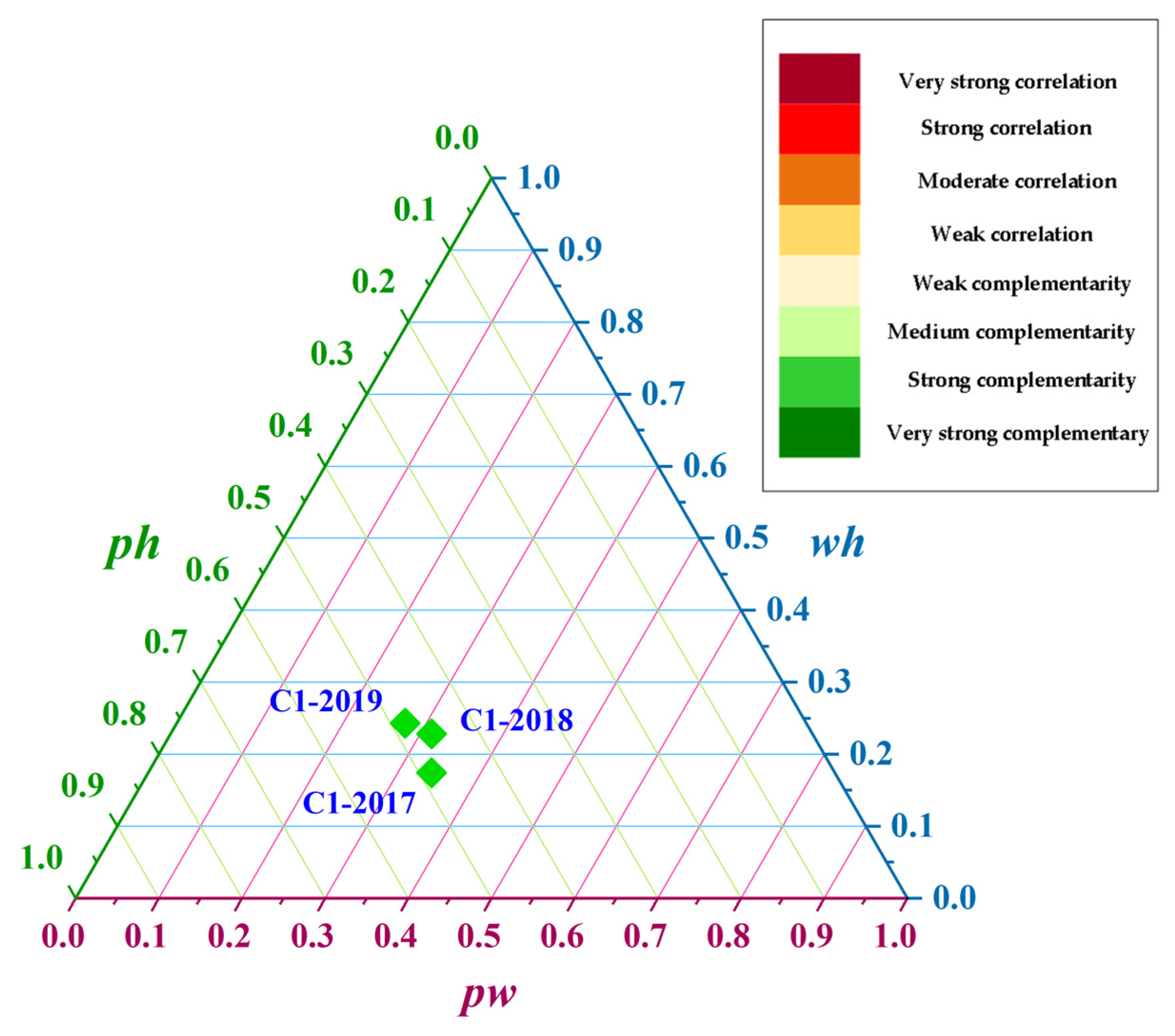
4.1. Analysis of Wind-Power–Photovoltaic-Power–Hydropower Complementary Characteristics at the Annual Scale

The output data of wind power, photovoltaic power, and hydropower from 2017 to 2019 are selected for complementary characteristic calculation and analysis; the results are shown in

Table 2. The complementary characteristics of the complementary combination 1 based on yearly data.

Year	Complementary Vector c	Spatial Optimal Solution $\mathit{L}\left(\mathit{c}\right)$	Total Complementary Index ${\mathit{k}}_{\mathit{t}}\left(\mathit{c}\right)$
2019	−0.693ph + 0.036pw + 0.148wh	1.246	77.96%
2018	−0.535ph − 0.524pw + 0.237wh	1.089	84.93%
2017	−0.611ph − 0.134pw + 0.420wh	1.338	73.87%

and

Table 3. The complementary characteristics of the complementary combination 2 based on yearly data.

Year	Complementary Vector c	Spatial Optimal Solution $\mathit{L}\left(\mathit{c}\right)$	Total Complementary Index ${\mathit{k}}_{\mathit{t}}\left(\mathit{c}\right)$
2019	−0.355ph − 0.126pw + 0.148wh	1.334	74.07%
2018	−0.612ph − 0.375pw + 0.237wh	1.125	83.33%
2017	−0.421ph − 0.158pw + 0.420wh	1.421	70.20%

. Figure 4 and Figure 5 show the total complementarity level in the three years, and the contribution of the three complementary combinations of wind-power–photovoltaic-power, photovoltaic-power–hydropower, and wind-power–hydropower to the total complementarity index.

Due to the different output of renewable energy in different years, there are specific differences in the complementary characteristics in different years. The complementary index shows that the wind-power–photovoltaic-power–hydropower total complementary characteristics of C1 and C2 are both strongly complementary in these three years, and the difference between the complementary indexes is slight. This means that the spatial difference brought by photovoltaic power stations has little impact on the total complementary index for the annual scale.

4.2. Analysis of Wind-Power–Photovoltaic-Power–Hydropower Complementary Characteristics at the Monthly Scale

The output data of wind power, photovoltaic power, and hydropower in the 12 months of 2019 are selected for complementary characteristic calculation and analysis; the results are shown in

Table 4. The complementary characteristics of the complementary combination 1 based on monthly data.

Month	Complementary Vector c	Spatial Optimal Solution $\mathit{L}\left(\mathit{c}\right)$	Total Complementary Index ${\mathit{k}}_{\mathit{t}}\left(\mathit{c}\right)$
1	−0.356ph + 0.041pw − 0.175wh	1.255	77.56%
2	−0.403ph − 0.119pw + 0.871wh	1.675	58.91%
3	0.858ph + 0.362pw + 0.433wh	2.327	29.93%
4	0.294ph − 0.478pw − 0.337wh	1.340	73.80%
5	0.375ph + 0.093pw + 0.617wh	2.043	42.56%
6	0.114ph + 0.195pw − 0.392wh	1.477	67.69%
7	0.639ph − 0.286pw − 0.565wh	1.394	71.38%
8	0.451ph − 0.129pw + 0.704wh	2.013	43.87%
9	0.267ph − 0.082pw − 0.415wh	1.385	71.78%
10	0.339ph − 0.383pw − 0.069wh	1.444	69.18%
11	0.594ph + 0.061pw − 0.288wh	1.684	58.51%
12	−0.383ph + 0.144pw − 0.279wh	1.241	78.18%

and

Table 5. The complementary characteristics of the complementary combination 2 based on monthly data.

Month	Complementary Vector c	Spatial Optimal Solution $\mathit{L}\left(\mathit{c}\right)$	Total Complementary Index ${\mathit{k}}_{\mathit{t}}\left(\mathit{c}\right)$
1	−0.274ph − 0.121pw − 0.175wh	1.270	76.91%
2	−0.525ph − 0.263pw + 0.871wh	1.542	64.82%
3	0.641ph − 0.011pw + 0.433wh	2.032	43.04%
4	0.556ph − 0.452pw − 0.337wh	1.384	71.84%
5	0.272ph − 0.081pw + 0.617wh	1.904	48.71%
6	0.305ph − 0.149pw − 0.392wh	1.382	71.91%
7	0.512ph + 0.037pw − 0.565wh	1.492	67.02%
8	0.219ph − 0.663pw + 0.704wh	1.630	60.89%
9	0.369ph − 0.152pw − 0.415wh	1.401	71.07%
10	0.291ph − 0.476pw − 0.069wh	1.373	72.31%
11	0.407ph − 0.196pw − 0.288wh	1.462	68.38%
12	−0.517ph − 0.021pw − 0.279wh	1.092	84.82%

. Figure 6 and Figure 7 show the total complementarity level in the 12 months, and the contribution of the three complementary combinations of wind-power–photovoltaic-power, photovoltaic-power–hydropower, and wind-power–hydropower to the total complementarity index.

There are extreme differences in the complementary characteristics of different months. In C1, there is strong complementarity in January, April, June, July, September, October, and December; medium complementarity in February, May, and August; and weak complementarity in March and November. In C2, except for March and May, which show moderate complementarity, other months show strong complementarity. This means that compared with C1, C2, with a 500 km distance between the photovoltaic power station and the wind farm, is more complementary on a monthly scale.

This result proves the effect of spatial distance on the multi-energy complementarity analysis: the farther the spatial distance between different power stations, the stronger the complementarity between them. This phenomenon is mainly determined by the meteorological factors in the study area.

Take wind power and photovoltaic for example: when the wind speed is high, the wind power output will increase, and the clouds in the sky will also be blown away by the strong wind. The photovoltaic will be affected, and the output will also increase. When the wind speed is low, the wind power output is low, and the weak wind may not disperse the clouds in the sky. The clouds will affect the photovoltaic power, and the output will be reduced or have inevitable volatility. Therefore, in C1, apoplexy and photovoltaic power show correlation rather than complementarity.

In C2, the photovoltaic power station is far from the wind farm. In strong windy weather, the wind power output increases. However, it may still be cloudy or cloudy near the photovoltaic power station, and the output of the photovoltaic power station may decrease. When the wind speed is low, the wind power output drops, but it may still be sunny near the photovoltaic power station, and the output increases. Since the output of the photovoltaic power generation will not change with the change of wind speed in the extended region of wind power, the relationship between wind power and photovoltaic power is more complementary.

On the monthly scale, C2’s complementarity is better than C1. Although the photovoltaic power station of C2 is far away from C1, C2 and C1 are still located in the upper reaches of the Yellow River. Therefore, C2 and C1 still have relatively similar monthly correlation changes. In both combinations, the smallest complementary index appeared in March. This is because the wind and photovoltaic power generation began to pick up in March due to climate change, whereas the hydropower generation also began to rise due to the ice melting in the upper reaches of the Yellow River, causing the three to be more correlated. Therefore, the total complementary index in March is the lowest. However, after entering April, photovoltaic and hydropower generation continued to increase, whereas wind power began to decrease due to the impact of the climate, so it showed better complementarity. The largest complementary index appeared in December because the photovoltaic and wind power generation was relatively high in that month, whereas hydropower generation was gradually declining because of the dry season, so the three were highly complementary. The best complementary index on the monthly scales was improved by 8.49%.

4.3. Analysis of Wind-Power–Photovoltaic-Power–Hydropower Complementary Characteristics at the Daily Scale

To more intuitively describe the complementary characteristics under the daily scale, this section selects the 24-h output data of each energy day in April, July, September, and December with better complementary characteristics in the two combinations. It picks one day on both sunny and rainy days, for a total of eight groups of data for analysis. The results are shown in

Table 6. The complementary characteristics of the complementary combination 1 based on daily data.

Day	Complementary Vector c	Spatial Optimal Solution $\mathit{L}\left(\mathit{c}\right)$	Total Complementary Index ${\mathit{k}}_{\mathit{t}}\left(\mathit{c}\right)$
S1	−0.005ph + 0.564pw − 0.177wh	1.691	58.18%
R1	0.080ph + 0.434pw − 0.126wh	1.694	58.04%
S2	−0.467ph + 0.125pw − 0.391wh	1.134	82.96%
R2	−0.171ph − 0.038pw − 0.249wh	1.271	76.84%
S3	0.263ph + 0.131pw − 0.087wh	1.654	59.84%
R3	0.192ph + 0.212pw − 0.153wh	1.626	61.09%
S4	−0.723ph − 0.286pw + 0.397wh	1.194	80.27%
R4	−0.496ph − 0.129pw + 0.351wh	1.363	72.76%

and

Table 7. The complementary characteristics of the complementary combination 2 based on daily data.

Day	Complementary Vector c	Spatial Optimal Solution $\mathit{L}\left(\mathit{c}\right)$	Total Complementary Index ${\mathit{k}}_{\mathit{t}}\left(\mathit{c}\right)$
S1	−0.165ph + 0.378pw − 0.177wh	1.518	65.87%
R1	−0.013ph + 0.587pw − 0.126wh	1.724	56.71%
S2	−0.561ph − 0.024pw − 0.391wh	1.012	88.36%
R2	−0.203ph + 0.151pw − 0.249wh	1.350	73.36%
S3	−0.217ph − 0.036pw − 0.087wh	1.330	74.22%
R3	−0.183ph + 0.327pw − 0.153wh	1.496	66.87%
S4	−0.492ph + 0.126pw + 0.397wh	1.516	65.98%
R4	−0.721ph − 0.307pw + 0.351wh	1.162	81.71%

; S represents the sunny day, and R represents the rainy day. Figure 8 and Figure 9 show the daily total complementarity level and the contribution of the three complementary combinations of wind-power–photovoltaic-power, photovoltaic-power–hydropower, and wind-power–hydropower to the total complementarity index.

There are great differences in the complementary characteristics of different days. In C1, there is strong complementarity in S2, R2, R3, S4, and R4, and medium complementarity in S1, R1, and S3. In C2, except for R1, which shows moderate complementarity, the other days all show strong complementarity. This means that compared with C1, C2 is more complementary on a daily scale.

As with the results in the complementarity analysis on the monthly scale, the daily scale results also prove that the farther the spatial distance between different power stations, the stronger the complementarity is between them. However, contrary to C2 and C1 on the monthly scale, there is still a relatively similar correlation change law. In the study of the daily scale, the change law of the total complementarity index of C1 and C2 on the same date is different, with significant differences. This is because the output curves of the two photovoltaic power stations with large geographical differences are significantly different daily. Whether on sunny or rainy days, the differences in the complementary characteristics of photovoltaic-power–wind-power and photovoltaic-power–hydropower ultimately affect the total complementary index.

The complementary characteristics of the daily data on S1, R1, S3, and R3 are lower than on other days. This is because these days are in April and September, which are in the flood season, and hydropower generates a large amount of electricity during the day. However, photovoltaic and hydropower show no or only weak complementarity on sunny or rainy days, affecting the overall complementary characteristics. The largest complementary index appeared in S2 because this day belongs to June, which is in the rainy season on the upper reaches of the Yellow River. As such, the weather frequently fluctuates during the day, and photovoltaic and wind power show strong volatility, enhancing the overall complementarity. The best complementary index on the daily scales was improved by 6.51%.

The effect of spatial distance on the multi-energy complementarity analysis proves that the farther the spatial distance between different power stations, the stronger the complementarity is between them. The analysis of wind-power–photovoltaic-power–hydropower complementary characteristics at the annual, monthly, and daily time scales shows significant differences in complementary characteristics under different time scales. The smaller the time scale is, the more pronounced the difference in the complementary characteristics is.

5. Conclusions

This paper combines the traditional correlation coefficient, three-dimensional vector, and compromise planning, and proposes a method to evaluate the complementarity of three energy sources at the same time. The method is verified in the largest renewable energy base in the upper reaches of the Yellow River in Qinghai Province, China. The results show that the process proposed in this paper can intuitively evaluate the overall and partial complementary characteristics of three energy sources. Moreover, to better evaluate spatial distance’s impact on complementary characteristics, this paper selects two photovoltaic power stations more than 500 km apart to study complementary characteristics at different time scales. The results prove that the farther the spatial distance between different power stations, the stronger the complementarity is between them. When the distance of the photovoltaic power station is longer, the best complementary index on the monthly and daily scales was improved by 8.49% and 6.51%. These results can provide a reference for the design and planning stage of large-scale renewable energy complementary systems, and can provide guidance for the operation and scheduling of multi-energy complementary systems.

Based on the existing wind–light–water multi-energy complementarity, the following work will focus on further considering the impact of spatial distance on the complementary characteristics. We will select wind farms, photovoltaic power plants, and hydropower stations with greater distances for analysis. Moreover, we will investigate the impact of multi-energy complementary systems using other energy sources, such as battery energy storage, air energy storage, biomass energy, and so on, on the overall complementary characteristics and stability.