A Hybrid Forecast Model for Household Electric Power by Fusing Landmark-Based Spectral Clustering and Deep Learning

Abstract

Household power load forecasting plays an important role in the operation and planning of power grids. To address the prediction issue of household power consumption in power grids, this paper chooses a time series of historical power consumption as the feature variables and uses landmark-based spectral clustering (LSC) and a deep learning model to cluster and predict the power consumption dataset, respectively. Firstly, the investigated data are reshaped into a matrix and all missing entries are recovered by matrix completion. Secondly, the data samples are divided into three clusters by the LSC method according to the periodicity and regularity of power consumption. Then, all samples in each cluster are expanded via bootstrap aggregating technique. Subsequently, a combination of a convolutional neural network (CNN) and a long short-term memory (LSTM) is employed to predict power consumption. The goal of CNN is to extract the features from input data in sequence learning, and LSTM aims to train and predict the power consumption. Finally, the forecasting performance of the LSC–CNN–LSTM is compared with several other deep learning models to verify its reliability and effectiveness in the field of household power load. The experimental results show that the proposed hybrid method is superior to other state-of-the-art deep learning techniques in forecasting performance.

1. Introduction

Environmental protection and low-carbon economy have gradually become the focus of attention, and the exploitation of energy has gradually changed to the direction of sustainability [1]. Energy consumption is an important factor in economic benefits, energy conservation and emission reduction contribute to the realization of social sustainable development. The role of electricity in energy supply has been gradually strengthened. Grasping the development trend of energy and electricity in the future has become a necessary way for economic growth and environmental protection. Correctly predicting household electricity consumption on the power grid is of great significance for energy transformation and the pursuit of sustainable development goals [2]. With economic development and population growth, global power consumption has increased significantly. Accurate power consumption prediction is very important for energy supply, power dispatching and distribution, capital investment and market research management [3]. More and more scholars devote themselves to the research of accurate and reliable energy consumption prediction methods. In essence, energy consumption prediction is a typical time series problem, including univariate prediction and multivariate prediction. Due to the uncertainty and volatility of power data, the traditional machine learning methods cannot predict power consumption well. In contrast, the deep learning techniques can achieve higher accuracy. For the problem of power consumption prediction, numerous related literatures have investigated abundant prediction models based on machine learning or even deep learning. Summarizing the relevant literature, the prediction models for power consumption are roughly divided into three categories: statistical methods, machine learning techniques [4,5,6,7] and hybrid models [8,9,10,11,12,13,14].

The first category focuses on the statistical analysis of historical time series data with different features, and the identification of the relationship among variables. The classical statistical learning methods mainly consist of the Markov process, regression model, exponential smoothing model, autoregressive model (AR), moving average model (MA), autoregressive moving average model (ARMA), autoregressive comprehensive moving average model (ARIMA) and so on [15]. These methods have the merits of fast calculation speeds and strong interpretability in predicting energy generation and power consumption. However, they cannot deal with sudden non-stationary data in general. More specifically, power consumption data are prone to be influenced by the seasons, the working day and other factors. Hence, this high variability can greatly reduce the prediction accuracy of statistical learning methods. The machine learning models can learn the complex nonlinear relationships and other relevant parameters in time series. Generally, these advanced learning models are superior to those statistical learning methods because of their powerful representation ability.

With the maturity of artificial intelligence technology, machine learning models have been widely applied in the community of energy generation and power consumption [16,17,18]. These models can effectively extract high-dimensional complex features and construct nonlinear mapping directly from input to output. Machine learning models adopted in the power consumption mainly include support vector machines (SVM) [19], support vector regression (SVR) [20,21], decision trees and artificial neural network (ANN) [22,23]. In the early stage of ANN, the shallow network construction is easier to implement and thus is widely used. The number of hidden layers in a shallow neural network is relatively small to avoid over-fitting, falling into a local minimum and gradient disappearance. One possible disadvantage of the aforementioned shallow topology is that the features contained in the data may not be completely extracted. As a result, the prediction accuracy needs to be further improved.

Deep learning techniques have emerged and achieved a rapid development with the continuous improvement of computer hardware, software and big data technology. So far, the boom of deep neural network technology has bred massive deep learning models, including deep belief network [24], convolutional neural network (CNN), long short-term memory (LSTM) [25,26], generative adversarial network, deep residual network [27], etc. As a branch of neural networks, a CNN has also been employed in time series in recent years. Compared with fully connected network, a CNN has advantages in fewer parameters and lower complexity. In addition, LSTM is a variant of a recurrent neural network (RNN), and it considers feedback connections to update the state of previous input neurons. The main difference between RNN and LSTM is that the latter has a long-term memory unit, which overcomes the disadvantage of unstable gradients in long-term dependent sequences. Nowadays, the LSTM model has been extensively applied in power system [28,29,30].

The hybrid methods concentrate the advantages of physical methods and data-driven methods, and they are widely utilized in building, household and urban power load forecasting. Yang et al. [31] explored the potential of hybrid models based on extreme learning machines, RNN, SVM and multi-objective particle swarm optimization (MOPSO) in multi-step load forecasting. The experimental results in [31] showed that the combined prediction model has higher prediction accuracy than the single model. Deep learning methods have also been extensively adopted in multi-step advance energy generation and power load forecasting [32,33]. In [20], an integration of generalized RNN and SVM was proposed to predict power demand, and it ensured the accuracy of prediction results and the robustness of the model. In [34], a power consumption prediction method was developed based on bidirectional LSTM (BiLSTM) and ANN, and it was enhanced with a multiple simultaneously decreasing delays approach coupled with function fitting neural networks. The hybrid method in [34] was also employed to predict the total power consumption of business center consumers and refrigerator storage room. Wu et al. [35] explored the CNN–LSTM–BiLSTM model with attention mechanism to predict short-term power load. Furthermore, the combination of the clustering method and deep learning model has also been comprehensively studied in power system prediction [36,37], such as the energy consumption based on k-means clustering [38,39], residential power load [40] and residential and small commercial building power demand by means of k-nearest neighbor [41].

In the power system, the accurate prediction of energy generation and power consumption has increasingly become a research hotspot. Various methods and technologies have been proposed to predict the energy generation, power demand or consumption, so as to provide a basic guarantee for the safe and stable operation in the power grid.

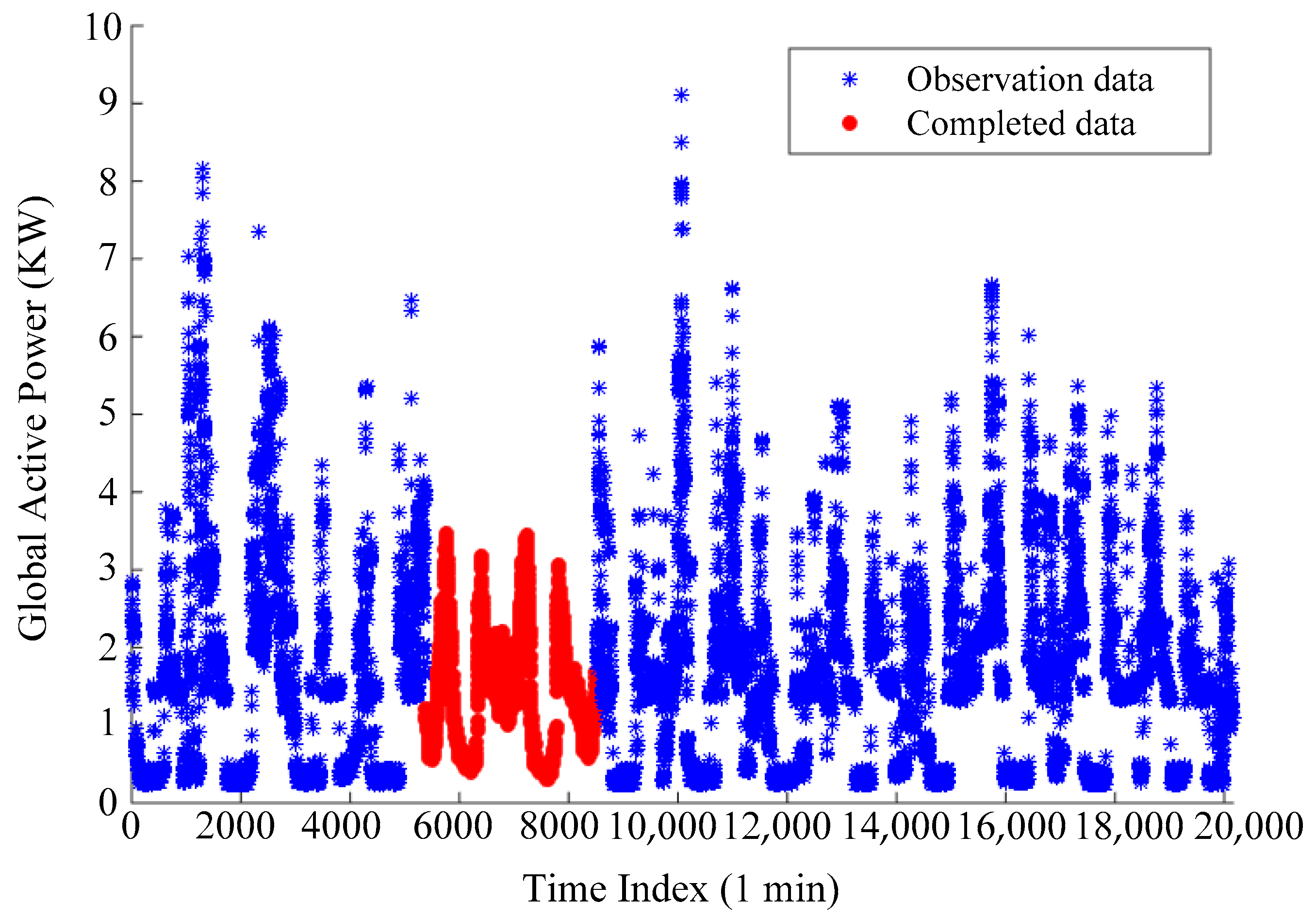
The aim of this paper is to forecast the household electric power through fusing landmark-based spectral clustering (LSC) and deep learning. Firstly, the missing values are recovered by matrix completion. Then, the linear normalization is employed to guarantee that the features are scaled in a proper order of magnitude. Next, household electric power samples are partitioned by LSC, where LSC is a scalable clustering method in massive datasets. Ultimately, a deep learning model is established by combining the advantages of CNN and LSTM. As a subsequence, a hybrid of LSC and deep learning is proposed for household electric power forecast.

The remaining structure of the paper is organized as follows. Section 2 elaborates on the investigated dataset, reviews methods for data preprocessing and provides a framework of the hybrid model. Section 3 introduces landmark-based spectral clustering and several deep learning techniques and proposes the LSC–CNN–LSTM model. The experimental results and analysis are discussed in Section 4. Finally, the conclusions are drawn in Section 5.

2. Materials and Methods

2.1. Dataset

Individual Household Electric Power Consumption (IHEPC), a dataset from UCI machine learning repository, is studied in this paper. It collected the power consumption of a family in Paris, France, from 17 December 2006 to 20 November 2010. There exist seven attributes in IHEPC, including global active power, reactive power, voltage, global intensity, kitchen active energy, laundry active energy, electric water heater and air conditioning active energy. Among them, the first attribute measures the total consumption of household electricity. The above attributes are recorded with a one-minute sampling rate, so they are arranged by a multivariable time series in essence. Without loss of generality, this paper only investigates the global active power. This attribute contains some missing entries, and the proportion of missing values is nearly 7.51%. For more complex power consumption behavior, more attributes can be considered further. The annual change trend of global active power is shown in Figure 1, where GAP is the abbreviation of global active power. It can be seen from this figure that the duration of consecutive missing data is different, and the missing values are concentrated in April 2007, June 2009 and January, March, August and September 2010. The longest time span of consecutive missing data is about 5 days.

Figure 2 shows the global active power with 20-min temporal resolution in June 2008. From the figure we can see that there is an approximate periodicity in weeks. The power consumption at the weekend reaches the peak value within a week and that on weekdays is less in most cases.

2.2. Data Preprocessing

2.2.1. Matrix Completion

The traditional interpolation methods are not suitable for the case of consecutive missing data. To recover all missing values in global active power, this part will resort to matrix completion, a promising signal processing technique [42]. Suppose that the maximum time span for consecutive missing elements is less than $O$ weeks. Let $D$ be the total number of weeks in IHEPC. For concise description, let us further assume that $D=OP$, where $P$ is a positive integer.

Let ${\mathit{v}}_i$ be a column vector recording the household electric power in the i-th week, $i=1,2,\dots ,D$. Therefore, the original data can be rewritten as a matrix

$$\mathit{V}=\left[\begin{array}{cccc}{\mathit{v}}_1& {\mathit{v}}_{O+1}& \cdots & {\mathit{v}}_{(P-1)O+1}\\ {\mathit{v}}_2& {\mathit{v}}_{O+2}& \cdots & {\mathit{v}}_{(P-1)O+2}\\ ⋮& ⋮& \ddots & ⋮\\ v_O& {\mathit{v}}_{2O}& \dots & {\mathit{v}}_{PO}\end{array}\right]$$

(1)

When $P$ is a relatively large number, the new data matrix $\mathit{V}$ is approximately low rank in view of its construction mode. For a given real matrix $\mathit{V}$, the nuclear norm ${‖\mathit{V}‖}_{\ast }$ is defined as the sum of its singular values [42]. The two-dimensional index set $\Omega$ is introduced to represent the subscript of the known elements in matrix $\mathit{V}$. Thus, a projection operator $T_{\Omega }(\cdot )$ is defined as follows: if $(i,j)\in \Omega$, then $T_{\Omega }(v_{ij})=v_{ij}$; otherwise, $T_{\Omega }(v_{ij})=0$.

Under mild conditions, all missing elements can be accurately recovered by solving a nuclear norm minimization problem, also called a matrix completion [42]. Mathematically, we establish the following optimization problem:

$$\underset{\tilde{\mathit{V}}}{\min }{‖\tilde{\mathit{V}}‖}_{\ast }, \mathrm{s}.\mathrm{t}. T_{\Omega }(\tilde{\mathit{V}})=T_{\Omega }(\mathit{V})$$

(2)

The optimal solution of the above problem is denoted by ${\mathit{V}}^{*}$.

The vectorization of ${\mathit{V}}^{*}$ is the completed time series of global active power. Based on this, we increase the sampling period of global active power to improve stability and reduce computational complexity. Concretely speaking, an hourly power consumption is synthetized by adding the values every 60 min, which means that the temporal resolution is changed from one minute to one hour. As a result, a new hourly power consumption dataset is created.

2.2.2. Data Normalization

In the community of machine learning and data science, data normalization is an indispensable component, and it is conducive to promote the convergence speed and effect. This normalization process is extremely essential to perform forecasting, and it is also beneficial to improve the prediction accuracy.

In this paper, the linear normalization method, also known as deviation standardization, is employed to process the global active power data. Let $x_{\min }$ and $x_{\max }$ be the minimum and maximum values of all observations, respectively. An attribute value $x$ can be normalized to the interval $[0,1]$ as follows:

$$x_{\mathrm{std}}=\frac{x-x_{\min }}{x_{\max }-x_{\min }}$$

(3)

Of course, other interval $[a,b]$ is easily obtained by scale transformation:

$$x_{\mathrm{scaled}}=x_{\mathrm{std}}\times (b-a)+a$$

(4)

The goal of normalization is to eliminate the influence of dimensions on different attributes. Simultaneously, it can be instrumental in more accurate training and prediction of neural network.

2.2.3. Samples Generation

In machine learning and deep learning, the number of training samples is expected to be large enough for the purpose of avoiding overfitting. The time series is represented by $\{l_1,l_2,\dots ,l_{N^{\prime }}\}$, where $N^{\prime }$ is the number of time stamps. The sliding windows with width $d$ and the sliding step size $s$ are selected to intercept the sequence data, and the dimensionality of output is set to $h$. In other words, the previous $d$ hours are employed to predict the next $h$ hours, as shown in Figure 3 for the case $s=1$. The input–output paired samples are constructed as follows:

Input features: ${\mathit{x}}_i={(l_i,l_{i+1},\dots ,l_{i+d-1})}^{\mathrm{T}}$.

Output features: $y_i={(l_{i+d},l_{i+d+1},\dots ,l_{i+d+h-1})}^{\mathrm{T}}$.

Input–output pairs: ${\left\{\right({\mathit{x}}_i,y_i)\}}_{i=1}^N$, where $N=N^{\prime }-d-h+1$.

2.3. Construction of the Hybrid Model

The hybrid model presented in this paper is mainly divided into three parts. Taking the global active power of household electricity as the studied object, the first part adopts matrix completion to recover the missing values. In the second part, a large scale spectral clustering with landmark-based representation is harnessed to cluster the generated samples, and the bootstrap aggregating is used to resample on each cluster to ensure that the number of new samples is consistent with that of original samples. A deep learning model by combining CNN and LSTM is proposed by carrying out the prediction in the last part. The detailed flow chart of the proposed hybrid model is illustrated in Figure 4.

3. A Deep Learning Framework by Combining LSC, CNN and LSTM

3.1. Landmark-Based Spectral Clustering

Spectral clustering is a kind of clustering method based on matrix decomposition [43]. Compared with other algorithms, spectral clustering usually produces better experimental performance because it considers the manifold structure of samples instead of Euclidean space. A key process in spectral clustering is calculating the eigenvectors of Laplacian matrix constructed by a similarity matrix. However, the eigen-decomposition has high computational complexity. Hence, the unscalable clustering method is limited in large scale data applications.

Landmark-based spectral clustering (LSC) can effectively deal with the issue of large scale samples [44]. The basic principle of LSC is to design an effective eigen-decomposition method of a Laplace matrix by means of constructing a novel graph. In implementation, $p$ representative data points are firstly selected as landmarks and each sample in the original data is approximately represented by the sparse linear combinations of these landmarks, where $p\ll N$, and $N$ is the number of samples. More specially, the sparse representation coefficients are directly obtained through the landmark-based representation matrix.

Matrix decomposition attempts to compress data by seeking a set of basis vectors and thus each data point is written as a linear combination of the bases [44]. Given the samples matrix $\mathit{X}=(x_1,x_2,\dots ,x_N)\in {\Re }^{d\times N}$, it is approximately decomposed into the product of two low-rank matrices:

$$\mathit{X}\approx \mathit{U}\mathit{Z}$$

(5)

where the base matrix $\mathit{U}\in {\Re }^{d\times p}$ and the coefficients matrix $\mathit{Z}\in {\Re }^{p\times N}$. As a basis vector, each column of $\mathit{U}$ captures the high-dimensional features from the original samples space. Meanwhile, each column of $\mathit{Z}$ is the $p$-dimensional representation coefficient of the corresponding input instance under the new basis vectors. The difference between two matrices is frequently measured by the Frobenius norm ${‖\cdot ‖}_F$ of the residual. Hence, the optimal low-rank representation can be obtained by solving the following optimization problem:

$$\underset{U,Z}{{\displaystyle \min }}{‖X-UZ‖}_{\mathrm{F}}^2$$

(6)

The optimal coefficient matrix $\mathit{Z}$ in the above minimization problem is usually dense, which means that each sample is a linear combination of all bases. These dense coefficients may result in a negative effect on classification performance. Sparse coding in matrix decomposition is a popular method to overcome the aforementioned defect. Furthermore, a sparse regularization term is imposed on the objective function in Equation (6), and a new optimization problem is formulated as below:

$$\underset{U,Z}{{\displaystyle \min }}{‖X-UZ‖}_F^2+\alpha f(Z)$$

(7)

where $f$ is a function to evaluate the sparsity of each column in $\mathit{Z}$ and $\alpha$ is a tradeoff coefficient to control the sparsity penalty.

To simplify model and reduce the computational complexity, LSC takes the landmarks as the basis vectors, which means all elements in basis matrix $\mathit{U}$ are not variables. The landmarks can be randomly chosen from the samples set or acquired via k-means clustering algorithm, where all clustering centers are regarded as the landmarks.

For data point ${\mathit{x}}_i$, its estimated value is denoted by ${\widehat{\mathit{x}}}_i={\displaystyle {\sum }_{j=1}^p{z}_{ji}{\mathit{u}}_j}$, where ${\mathit{u}}_j$ is the $j$-th column of $\mathit{U}$ and $z_{ji}$ is an element in the $j$-th row and $i$-th column of $\mathit{Z}$. A natural assumption is that the closer ${\mathit{x}}_i$ is to ${\mathit{u}}_j$, the larger the value of $z_{ji}$ should be. Let $〈i〉$ be the index set composed by $r$ nearest neighbors of ${\mathit{x}}_i$ from ${\left\{{\mathit{u}}_j\right\}}_{j=1}^p$ and $r\ll p$. If $j\notin 〈i〉$, then $z_{ji}$ is set to 0; otherwise, the value of $z_{ji}$ is determined by the following formula:

$$z_{ji}=\frac{K({\mathit{x}}_i,{\mathit{u}}_j)}{{\displaystyle {\sum }_{j^{\prime }\in 〈i〉}K({\mathit{x}}_i,{\mathit{u}}_{j^{\prime }})}}$$

(8)

where $K(\cdot ,\cdot )$ is a kernel function. In practice, the Gaussian function or thermal kernel is a priority to recommend the kernel function:

$$K({\mathit{x}}_i,{\mathit{u}}_j)=\exp \left(-\frac{{‖{\mathit{x}}_i-{\mathit{u}}_j‖}_2^2}{2h^2}\right)$$

(9)

where $h$ is a fixed bandwidth. The value of $r$ restricts that $\mathit{Z}$ is a sparse matrix.

According to the sparse representation matrix $\mathit{Z}$ calculated from landmarks, the affinity matrix, also named as similarity matrix, can be obtained as follows:

$$\mathit{W}={\widehat{\mathit{Z}}}^{\mathrm{T}}\widehat{\mathit{Z}}$$

(10)

where $\widehat{\mathit{Z}}={\hat{\mathit{D}}}^{-1/2}\mathit{Z}$, $\hat{D}=\mathrm{diag}({\widehat{d}}_{11},{\widehat{d}}_{22},\dots ,{\widehat{d}}_{pp})$ is a $p$-order diagonal square matrix whose diagonal elements are the sum of each row of matrix $\widehat{\mathit{Z}}$, i.e., ${\widehat{d}}_{ii}={\displaystyle {\sum }_j{z}_{ij}}$.

The thin singular value decomposition is performed on matrix $\widehat{\mathit{Z}}$ and thus $\widehat{\mathit{Z}}=\mathit{A}\mathbf{\Sigma }{\mathit{B}}^{\mathrm{T}}$ is obtained, where $\mathbf{\Sigma }=diag({\sigma }_1,{\sigma }_2,\dots ,{\sigma }_p)$ and ${\sigma }_1\ge {\sigma }_2\ge \dots \ge {\sigma }_p\ge 0$ are singular values of $\widehat{\mathit{Z}}$. Denote $\mathit{A}=\left({\mathit{a}}_1,{\mathit{a}}_2,\dots ,{\mathit{a}}_p\right)\in {\Re }^{p\times p}$ and $B=\left({\mathit{b}}_1,{\mathit{b}}_2,\dots ,{\mathit{b}}_p\right)\in {\Re }^{N\times p}$, where ${\mathit{a}}_i$ is called left singular vector and ${\mathit{b}}_i$ is the right singular vector. It is easy to draw the following conclusions: each column of matrix $\mathit{B}$ is an eigenvector of matrix ${\widehat{\mathit{Z}}}^{\mathrm{T}}\widehat{\mathit{Z}}$, each column of matrix $\mathit{A}$ is an eigenvector of matrix $\widehat{\mathit{Z}}{\widehat{\mathit{Z}}}^{\mathrm{T}}$, and ${\sigma }_i{}^2$ is the $i$-th largest eigenvalue of ${\widehat{\mathit{Z}}}^{\mathrm{T}}\widehat{\mathit{Z}}$ or $\widehat{\mathit{Z}}{\widehat{\mathit{Z}}}^{\mathrm{T}}$. Furthermore, it holds that:

$${\mathit{B}}^{\mathrm{T}}={\mathbf{\Sigma }}^{-1}{\mathit{A}}^{\mathrm{T}}\widehat{\mathit{Z}}$$

(11)

The procedure of LSC is summarized in Algorithm 1.

Algorithm 1 LSC

input: ${\{{\mathit{x}}_i\in {\Re }^d\}}_{i=1}^N$: samples set, $c$: number of clusters, $p$: number of landmarks.

output: $c$ clusters after the clustering process.

1. Generate $p$ landmarks using k-means clustering or a random selection from ${\left\{{\mathit{x}}_i\right\}}_{i=1}^{\mathit{N}}$.

2. Construct the sparse affinity matrix $\mathit{Z}\in {\Re }^{p\times N}$ between data points and landmarks according to Equation (8) and normalize it by $\widehat{\mathit{Z}}={\widehat{\mathit{D}}}^{-1/2}\mathit{Z}$.

3. Calculate the first top $p$ eigenvectors of matrix $\widehat{\mathit{Z}}{\widehat{\mathit{Z}}}^{\mathrm{T}}$ and form a matrix $\mathit{A}=\left({\mathit{a}}_1,{\mathit{a}}_2,\dots ,{\mathit{a}}_p\right)$ by stacking them column by column.

4. Compute matrix $\mathit{B}=\left({\mathit{b}}_1,{\mathit{b}}_2,\dots ,{\mathit{b}}_p\right)$ through Equation (11).

5. Regard each row of matrix $\mathit{B}$ as a new data point and cluster them with k-means clustering or other algorithms to obtain the final result.

In Algorithm 1, the constructed samples matrix $\mathit{X}$ is used as the input of clustering. Each column of $\mathit{X}$ is regarded as an original sample, and all samples are eventually grouped into three clusters in our experiments. Under ideal conditions, the similarity of data points from the same cluster is high; otherwise, the similarity is low. The resulting three clusters are respectively adopted as the training set of deep neural network for prediction.

3.2. Bootstrap Aggregating

Generally, the number of training samples will decrease significantly owing to the utilization of LSC. However, all deep learning techniques require sufficient training samples. Under such circumstances, the proposed clustering method may lead to a risk of deteriorating overfitting. Meanwhile, fewer sample points will also seriously affect the prediction performance of deep learning. For these reasons, a sample augmentation strategy is proposed.

Bootstrap aggregating, also called as bagging, is a commonly-used ensemble learning method. For a given sample set, this method will generate a new sample set using a resampling technique. In the process of resampling, each point in original sample set is randomly selected according to the uniform distribution, and duplicate samples are permissible in the resulting set. Though the bootstrap aggregating, samples in each cluster can be augmented arbitrarily. For each cluster, this paper generates stochastically an updated sample set whose sample number is $N$.

Once each cluster is augmented, the prediction process will be executed based on deep learning methods. It is worth noting that the bootstrap aggregating technique allows us to fairly compare the experimental results before and after clustering, and simultaneous overfitting is alleviated to a certain extent. In addition, the data variability caused by bootstrap aggregating has a low risk of overfitting because it has little impact on batches.

3.3. Convolutional Neural Network

As a special case of a feedforward neural network, a convolutional neural network (CNN) owns the characteristics of convolution calculation and depth structure, and it has been one of the representative models among deep learning techniques. What is more, CNN can effectively learn the latent features from input data, respond to the surrounding units within the coverage, and have strong learning representation ability.

Although CNN is usually applied to extracting features on two-dimensional images, it also supports multiple one-dimensional input and is very suitable for a multi-step time series prediction. This paper will pay more attention to one-dimensional CNN, which mainly includes an input layer, several hidden layers and an output layer. Among them, the hidden layer consists of a convolution operator, pooling operator and full connection operator.

The first operator involves multiple convolution kernels and its function is to extract the features from the corresponding input. Each element of a convolution kernel represents a weight coefficient. The size of a convolution nucleus determines the size of a receptive field, and the step size controls the sliding length of the receptive field.

After feature extraction via the convolution operator, the output feature map will be transferred to the pooling operation for feature selection and information filtering. The effect of the pooling is to replace the single point results in the feature graph with the feature statistics of adjacent regions. The pooling area and the sliding size are, respectively, controlled by the pooling size and the step size, where the step is similar to that in the convolution kernel for the scanning feature graph.

The full connection operator is equivalent to the hidden layer in traditional feedforward neural network (FFNN). Both the convolution and pooling can extract the features from the input data, and the full connection is utilized to nonlinearly combine the extracted features to obtain the output. The prior layer of the output layer in CNN is usually the full connection.

An analytical diagram of one-dimensional convolution and pooling process is shown in Figure 5. The input vector with $d$ dimensions is operated with $k$ convolution kernels. In the later experiments, the size of convolution kernel and the step size are set to 3 and 1, respectively. Convolution operation is a process of continuously sliding weighted summation, where the height is set to 3. When the input sample is passed through the sliding window operation with $k$ convolution kernels, a matrix $\mathit{C}={(c_{ij})}_{(d-2)\times k}$ can be calculated through weighted summation:

$$c_{ij}=l_i{w}_{1j}+l_{i+1}{w}_{2j}+l_{i+2}{w}_{3j}i=1,2,\dots ,d-2;j=1,2,\dots ,k$$

(12)

The sliding window operation in pooling is similar to the convolution operation, and the pooling size is set to 2 in the experimental section. Pooling operator is a process of dimensionality reduction by continuously sliding the window with height 2 and width 1. Maximum pooling selects the largest value from the fixed region of interest as the output, where the region is obtained by convolution in the sliding window. After convolution and pooling operators, the previous feature matrix $\mathit{C}$ is eventually be transformed into another matrix $\mathit{P}={(p_{ij})}_{q\times k}$, where $p_{ij}=\max \{c_{2i-1,j},c_{2i,j}\}$, $q=(d-2)/2$.

3.4. Long Short-Term Memory

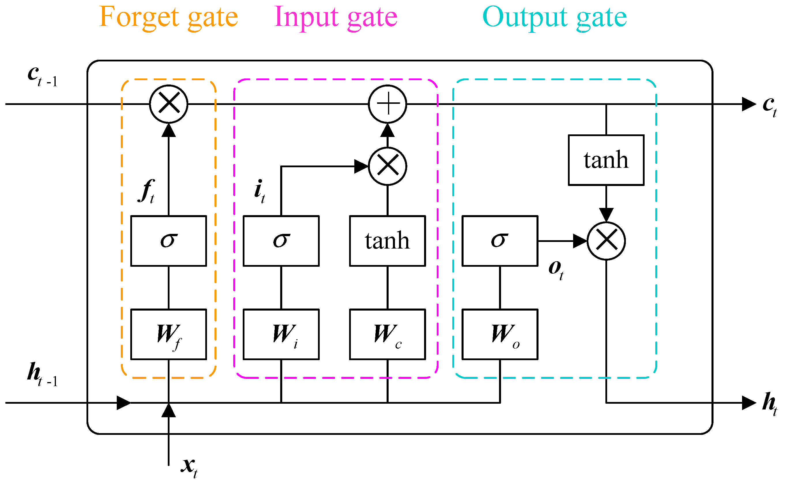
A recurrent neural network (RNN) carries the memory information from prior inputs and outputs, and it is especially suitable for the sequential data or time series data. As a popular variant of RNN, long short-term memory (LSTM) can overcome the problem of gradient disappearance and exploding by fusing self-connected gates in hidden cells. Figure 6 gives the architecture of an LSTM unit. There exist three types of gates in LSTM, i.e., input gate, forgetting gate and output gate. The first gate controls the input of new information in the memory cell. The second gate is response for whether previous information should be forgotten from memory cells. The last gate controls the output of information. The information is transmitted in the following order. The current information is first passed through the input gate to see whether there is input information. The second step is to judge whether the forgetting gate chooses to forget the information in the memory cell. Finally, the available information is further transmitted the output gate to judge whether to output the information at that moment.

Given input vector ${\mathit{x}}_t$ in LSTM unit at time $t$, the calculation process is shown in Equations (13)–(18):

$${\mathit{f}}_t=\sigma ({\mathit{W}}_{fh}{\mathit{h}}_{t-1}+{\mathit{W}}_{fx}{\mathit{x}}_t+{\mathit{b}}_f)$$

(13)

$${\mathit{i}}_t=\sigma ({\mathit{W}}_{ih}{\mathit{h}}_{t-1}+{\mathit{W}}_{ix}{\mathit{x}}_t+{\mathit{b}}_i)$$

(14)

$${\mathit{o}}_t=\sigma ({\mathit{W}}_{oh}{\mathit{h}}_{t-1}+{\mathit{W}}_{ox}{\mathit{x}}_t+{\mathit{b}}_o)$$

(15)

$${\tilde{\mathit{c}}}_t=\tanh ({\mathit{W}}_{ch}{\mathit{h}}_{t-1}+{\mathit{W}}_{cx}{\mathit{x}}_t+{\mathit{b}}_c)$$

(16)

$${\mathit{c}}_t={\mathit{f}}_t\circ {\mathit{c}}_{\mathit{t}-1}+{\mathit{i}}_t\circ {\tilde{\mathit{c}}}_t$$

(17)

$${\mathit{h}}_t={\mathit{o}}_t\circ \tanh (c_t)$$

(18)

where the notation $\circ$ indicates the Hadamard product, $\sigma (\cdot )$ is the sigmoid activation function and $\tanh (\cdot )$ is the hyperbolic tangent activation function. In Equations (13)–(15), ${\mathit{f}}_t$, ${\mathit{i}}_t$ and ${\mathit{o}}_t$ are, respectively, the forget gate, the input gate and the output gate; ${\mathit{W}}_{fh}$, ${\mathit{W}}_{ih}$ and ${\mathit{W}}_{oh}$ are the weight matrices of forget gate, input gate and output gate connecting the output of the previous unit, respectively; ${\mathit{W}}_{fx}$, ${\mathit{W}}_{ix}$ and ${\mathit{W}}_{ox}$ are the weight matrices of aforementioned three gates connecting the input of the current unit, respectively. In Equations (16)–(18), ${\tilde{\mathit{c}}}_t$, ${\mathit{c}}_t$ and ${\mathit{h}}_t$ are, respectively, the candidate values, the state vector and the output vector; ${\mathit{W}}_{ch}$ and ${\mathit{W}}_{cx}$ are the input weight matrices connecting the output of the previous unit, respectively. Moreover, ${\mathit{b}}_f$, ${\mathit{b}}_i$ and ${\mathit{b}}_o$ are the bias vectors of three gates, respectively, and ${\mathit{b}}_c$ is the input bias vector.

3.5. Integration of LSC, CNN and LSTM

LSC classifies the original samples into several groups. In general, samples in each group have lower model complexity than all samples, which means that the trained forecasting model tends to have higher performance. CNN has powerful ability in feature extraction and representation learning. In addition, LSTM has natural advantage to transmitting information in time series data. Combining the advantages of these three methods, this paper presents a hybrid forecasting model, called as LSC–CNN–LSTM. 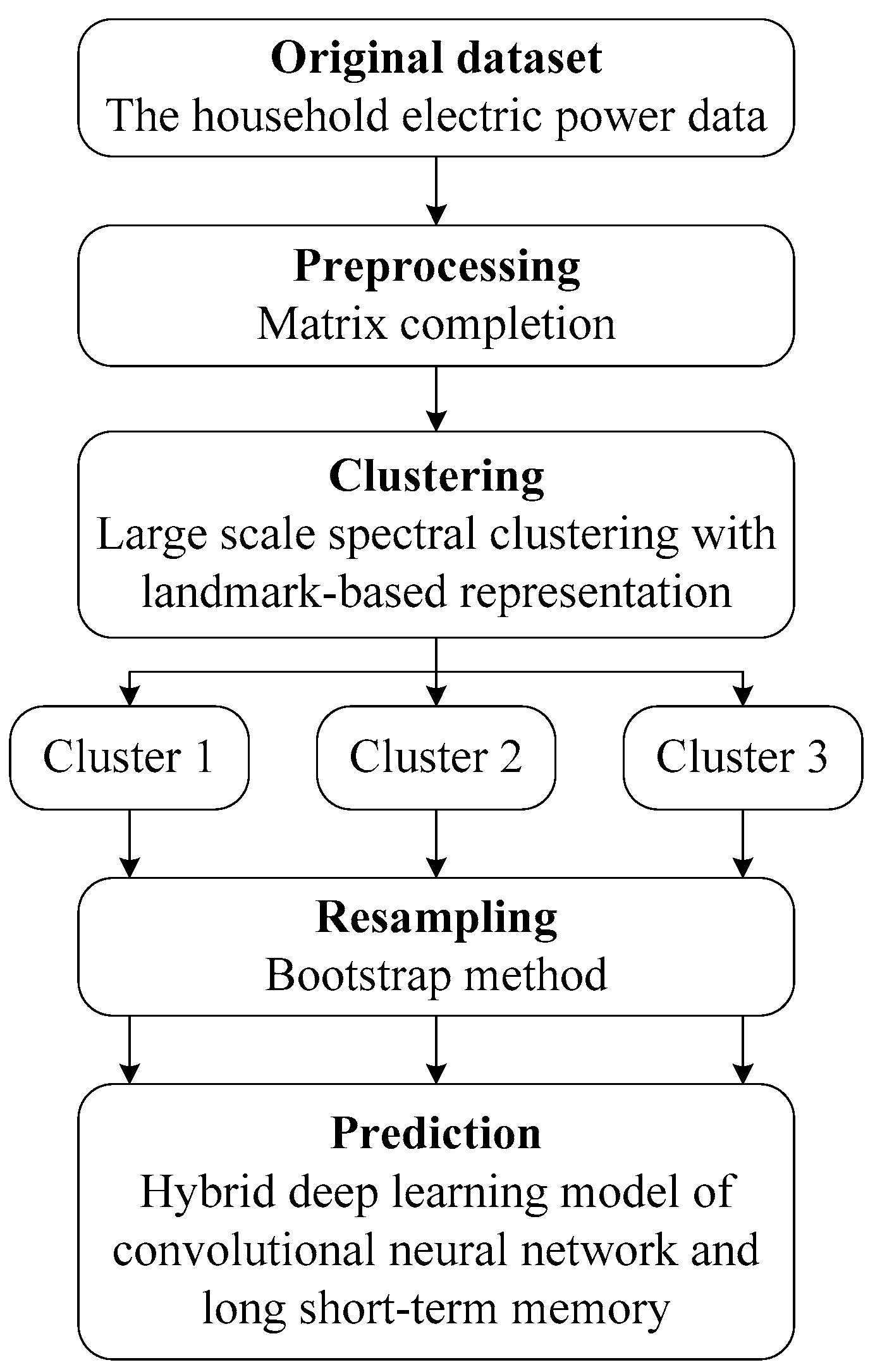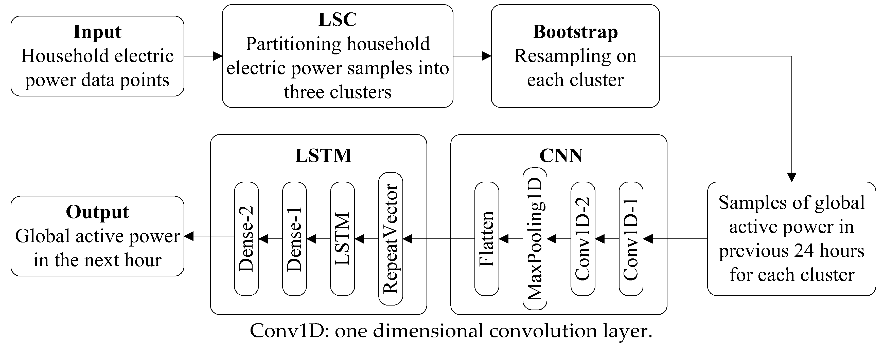Figure 7 sketches the framework of the proposed novel deep learning model. In this figure, the structure of LSC–CNN–LSTM mainly includes input feature vector module, large scale spectral clustering model, resampling module, CNN feature extraction module and sequence training prediction module.

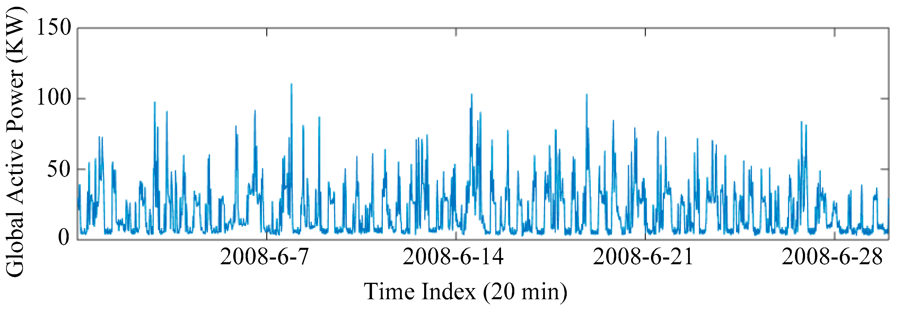
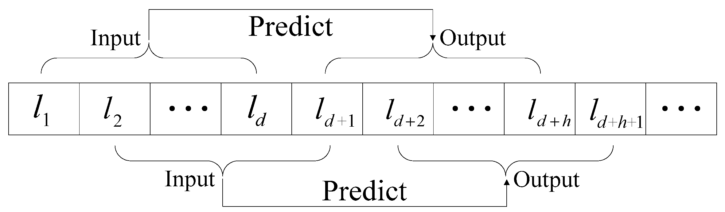
Samples generated by the global active power data are firstly passed on to the input feature vector module, and then all input samples are partitioned into three clusters through LSC. Subsequently, bootstrap aggregating is applied in each cluster to increase the number of samples. For each cluster, the global active power of household electricity in previous 24 h is used as the input of deep neural network. The feature extraction module in CNN mainly includes two one-dimensional convolution layers and a maximum pooling layer. Specifically, one-dimensional convolution can read the sequence input features and automatically learn the latent features. The first convolution layer establishes the feature map from the input sequence, and the second performs the same convolution operation on the feature map created by the first layer to enlarge its salient features. The maximum pooling layer simplifies the feature map obtained by convolution for the sake of dimensionality reduction. Finally, the reduced feature map is flattened into a long vector through leveling.

The purpose of the Repeat Vector is that it repeats the internal representation of the input sequence multiple times, and repeats once for each time step in the output sequence. The output of CNN is input into the LSTM unit. The subsequent sequence prediction module mainly consists of one LSTM layer and two full connection layers. The LSTM layer is connected by two fully connected layers. The fully connected layer makes a nonlinear transformation to the previously extracted features, extracts the correlation between features and maps them to the output space. The global active power of the next hour is ultimately obtained after feature extraction and sequence training prediction.

4. Results and Discussion

In this section, the proposed hybrid model is applied to the IHEPC dataset to realize the one-step prediction of global active power of household electricity. The experimental results are compared with other benchmark neural network models, including FFNN, CNN and LSTM. The prediction accuracies with and without LSC are compared.

4.1. Experimental Preparation and Settings

In matrix completion, $O$ is set to 2. As a result, the size of matrix ${\mathit{V}}^{*}$ is $7O\times P$. The rank of ${\mathit{V}}^{*}$ is assumed to be $r^{\prime }$,where $r^{\prime }\ll \min (7O,P)$. All missing values can be recovered by matrix completion technique since the sampling rate of the dataset is greater than $\left(7O\times P-r^{\prime }\right)\times r^{\prime }/\left(7O\times P\right)$. Taking January 2010 as an example, there are 3129 consecutive missing values between 12 January to 14 January. Figure 8 illustrates the complete data in that month, where the blue stars represent the observed values and the red filled circles are the recovered values. It can be seen from this figure that the matrix completion has preferable performance in recovering missing values. Moreover, this completion technique is conducive to suppressing large noise.

The task in this paper is to predict the global active power of household electricity in the next hour based on the previous 24 h. According to the construction method of samples, a total of 34,416 samples are generated. In the process of the learning model, the first 80% of samples are taken as the training set and the last 20% as the test set. Figure 9 shows the diagrammatic sketch of the division of sample set.

In LSC, all samples are partitioned into three clusters, and $p$ and $r$ are set to 1000 and 5, respectively.

Table 1. Parameter setting of each layer in the proposed hybrid model.

Type	Parameter	Value	Output Size
Conv1D-1	Kernels	32	22 × 32
	Kernel_size	3
	Activation function	relu
Conv1D-2	Kernels	32	20 × 32
	Kernel_size	3
	Activation function	relu
MaxPooling1D	Pooling_size	2	10 × 32
Flatten	-	-	320
RepeatVector	-	-	1 × 320
LSTM	Number of neurons	50	1 × 50
	Activation function	relu
	Return_sequences	True
Dense-1	Number of neurons	10	1 × 10
	Activation function	relu
Dense-2	Number of neurons	1	1 × 1

shows the parameter settings in each layer for the combined deep learning model. An input sample is firstly processed through two successive layers of one-dimensional CNN and one layer of maximum pooling operation is followed. The number of convolution kernels is set to 32, and the size of each kernel is 3. What is more, the rectified linear unit (relu) is chosen as the activation function in the convolutional module. After the first convolution operation, the input sample is converted to a 22 × 32 matrix. Through the second convolution operation, the above matrix is transformed into a 20 × 32 matrix. Ultimately, the feature matrix is further converted to a 10 × 32 matrix via the maximum pooling. The number of neurons in the LSTM unit is set to 50, and the relu is employed as the activation function. The number of neurons in two fully connected layers is set to 10 and 1, respectively.

The parameter settings for solving the deep neural network are shown in

Table 2. Parameter settings for solving the deep neural network.

Parameter	Setting
Optimizer	Adam
Loss function	Mean Square Error (MSE)
Batch size	40
Number of epochs	80

. Adam is selected as the optimizer of the network and mean square error (MSE) is the loss function to evaluate the learning performance. Furthermore, let the batch size be 40 and the number of epochs be 80.

Three commonly used evaluation indexes, the root mean square error (RMSE), the mean absolute error (MAE) and the determination coefficient ${\mathrm{R}}^{\mathrm{2}}$, are employed to quantitatively evaluate the prediction performance of the proposed model. Their calculation formulas are as follows:

$$\mathrm{R}\mathrm{M}\mathrm{S}\mathrm{E}=\sqrt{\frac{1}{n}{\displaystyle \sum _{i=1}^n{({\widehat{y}}_i-y_i)}^2}}$$

(19)

$$\mathrm{M}\mathrm{A}\mathrm{E}=\frac{1}{n}{\displaystyle \sum _{i=1}^n\left|{\widehat{y}}_i-y_i\right|}$$

(20)

$${\mathrm{R}}^{\mathrm{2}}=\frac{{\displaystyle \sum _{i=1}^n(y_i-\overline{y})}({\widehat{y}}_i-\overline{\widehat{y}})}{\sqrt{{\displaystyle \sum _{i=1}^n{(y_i-\overline{y})}^2}}\sqrt{{\displaystyle \sum _{i=1}^n{({\widehat{y}}_i-\overline{\widehat{y}})}^2}}}$$

(21)

where the scalar $y_i$ is the actual value corresponding to the $i$-th input instance, ${\widehat{y}}_i$ is the predicted value of $y_i$, $\overline{y}$ is the average value of the actual values, $\overline{\widehat{y}}$ is the average value of the predicted values and $n$ is the total number of samples.

4.2. Results Comparison without Clustering

This subsection will only consider the prediction performance of the CNN–LSTM model without clustering. FFNN, CNN and LSTM models are compared with the combination of CNN and LSTM. A hidden layer with 10 nodes is set in FFNN. The model of CNN concludes two layers of one-dimensional CNN and one layer of maximum pooling, two fully connected layers are followed. The number of convolution kernels is set to 32, the size of each kernel is 3 and the pooling size is 2. The LSTM model consists of one LSTM layer and two fully connected layers. The number of neurons in the LSTM unit is set to 50, and the activation function is relu. The number of neurons in the two fully connected layers is set to 10 and 1, respectively.

Figure 10 shows the training loss of the aforementioned four models in power consumption prediction. The training loss of FFNN model converges in advance and the iteration is stopped after 19 epochs, which effectively avoids overfitting and keeps the error relatively small. As can be seen from Figure 10, the training loss becomes small with the increasing of the number of epochs, and it drops sharply in the second epoch, which lead to the subsequent fluctuation changes that are relatively small. The higher the number of epochs, the smaller the loss drop. The loss gradually approaches a steady state when the epoch is relatively large. Compared with other methods, CNN–LSTM achieves the optimal RMSE within 80 epochs.

For four single models, three evaluation errors on the test set are shown in the first four rows of

Table 3. RMSE without and with clustering.

Model	Cluster 1	Cluster 2	Cluster 3	Average
FFNN	-	-	-	0.1535
CNN	-	-	-	0.1618
LSTM	-	-	-	0.1564
CNN–LSTM	-	-	-	0.1776
k-means–FFNN	0.1811	0.1506	0.1852	0.1723
k-means–CNN	0.1545	0.1472	0.1636	0.1551
k-means–LSTM	0.1627	0.1490	0.1651	0.1589
k-means–CNN–LSTM	0.0888	0.0995	0.0806	0.0896
LSC–FFNN	0.1294	0.1816	0.1714	0.1608
LSC–CNN	0.1165	0.1702	0.1589	0.1485
LSC–LSTM	0.1223	0.1801	0.1623	0.1549
LSC–CNN–LSTM	0.0392	0.1072	0.1040	0.0835

,

Table 4. MAE without and with clustering.

Model	Cluster 1	Cluster 2	Cluster 3	Average
FFNN	-	-	-	0.1065
CNN	-	-	-	0.1197
LSTM	-	-	-	0.1071
CNN–LSTM	-	-	-	0.1216
k-means–FFNN	0.1254	0.1003	0.1336	0.1198
k-means–CNN	0.1100	0.0999	0.1206	0.1102
k-means–LSTM	0.1126	0.1018	0.1168	0.1104
k-means–CNN–LSTM	0.0513	0.0608	0.0479	0.0533
LSC–FFNN	0.0855	0.1321	0.1131	0.1102
LSC–CNN	0.0773	0.1249	0.1075	0.1032
LSC–LSTM	0.0828	0.1272	0.1116	0.1072
LSC–CNN–LSTM	0.0240	0.0625	0.0622	0.0496

and

Table 5. ${\mathrm{R}}^2$ without and with clustering.

Model	Cluster 1	Cluster 2	Cluster 3	Average
FFNN	-	-	-	0.7406
CNN	-	-	-	0.7190
LSTM	-	-	-	0.7341
CNN–LSTM	-	-	-	0.6646
k-means–FFNN	0.7996	0.7536	0.7755	0.7762
k-means–CNN	0.8609	0.7672	0.8303	0.8195
k-means–LSTM	0.8420	0.7627	0.8290	0.8112
k-means–CNN–LSTM	0.9560	0.9008	0.9621	0.9396
LSC–FFNN	0.7695	0.7752	0.7842	0.7763
LSC–CNN	0.8217	0.8092	0.8188	0.8166
LSC–LSTM	0.8087	0.7878	0.8140	0.8035
LSC–CNN–LSTM	0.9813	0.9285	0.9304	0.9467

. It can be seen from the above tables that the RMSE of FFNN, CNN, LSTM and CNN–LSTM are 0.1535, 0.1618, 0.1564 and 0.1776, respectively; the MAE are 0.1065, 0.1197, 0.1071 and 0.1216, respectively; and the ${\mathrm{R}}^2$ are 0.7406, 0.7190, 0.7341 and 0.6646, respectively. According to these observations, FFNN and LSTM have better prediction performance than CNN and CNN–LSTM.

The last three days of the test set were selected to further compare the forecast results after inverse normalization. The RMSE of FFNN, CNN, LSTM and CNN–LSTM in these three days are 38.2275, 38.2686, 37.0078 and 40.6258, respectively; the MAE are 21.2063, 23.8025, 20.8860 and 23.8505, respectively; and the ${\mathrm{R}}^2$ are 0.6999, 0.7006, 0.7235 and 0.6593, respectively. The experimental results are also visualized in Figure 11. In this figure, the black curve is the actual observed value, and the others are the predicted values. It can be seen that the predicted value curves of these models are consistent with the actual observed value curve to a certain extent. From the evaluation indexes and prediction curves, LSTM yields the best prediction performance, and its prediction curve is closer to the actual curve.

4.3. Results Comparison with Clustering

Both k-means and LSC are adopted during the procedure of clustering, and the samples are classified into three clusters. Bootstrap aggregating is applied to expand samples in each cluster, which avoids overfitting to a certain extent and yields fair comparison. Subsequently, several deep learning models are employed to perform prediction in different clusters. Samples from the same cluster will be easier to train in general. Experiments are carried out separately via fusing the clustering method with machine learning or deep learning techniques. The prediction results with and without clustering are recorded and compared on test set.

For four single models, their combinations with clustering are, respectively, used to predict household electric power, and the evaluation errors are shown in Table 3, Table 4 and Table 5. With k-means clustering, the CNN–LSTM has the best performance among four models. On average, the RMSE of CNN–LSTM is 0.0896, the MAE is 0.0533 and the ${\mathrm{R}}^2$ is 0.9396. Hence, the performance of CNN–LSTM is greatly improved compared with other three models. With LSC, the RMSE values of three clusters in the CNN–LSTM model are 0.0392, 0.1072 and 0.1040, respectively, and the average is 0.0835; the MAE values are 0.0240, 0.0625 and 0.0622, respectively, and the average is 0.0496; and the ${\mathrm{R}}^2$ values are 0.9813, 0.9285 and 0.9304, respectively, and the average is 0.9467. In summary, two error evaluation indexes of CNN–LSTM with LSC are smaller than those without clustering in three clusters, and the ${\mathrm{R}}^2$ obtains the maximum value. As for running time, k-means clustering takes 6.6689 s and LSC is 2.4655 s faster than k-means clustering. Although k-means–CNN–LSTM has a better result in cluster 2 and cluster 3 in terms of RMSE and MAE, it is only slightly better and is not dominant in time. LSC–CNN–LSTM has obvious advantages in cluster 1 and has superiority in the overall accuracy. The experimental results show that the prediction accuracy can be effectively improved by using the CNN–LSTM model with LSC.

Similarly, the forecast results of the last three days (72 samples) for three clusters are, respectively, displayed to visualize the disparity between the actual value and the predicted value under different models with LSC. The evaluation errors of LSC–FFNN, LSC–CNN, LSC–LSTM and LSC–CNN–LSTM in these three days are shown in

Table 6. RMSE of different models with LSC in the last three days.

Model	Cluster 1	Cluster 2	Cluster 3	Average
LSC–FFNN	24.7004	36.1183	33.1139	31.3109
LSC–CNN	26.4603	33.1796	27.7059	29.1153
LSC–LSTM	28.0363	32.0900	32.4298	30.8520
LSC–CNN–LSTM	7.3222	21.3219	23.9670	17.5370

,

Table 7. MAE of different models with LSC in the last three days.

Model	Cluster 1	Cluster 2	Cluster 3	Average
LSC–FFNN	18.2412	27.5652	21.3021	22.3695
LSC–CNN	16.1984	26.1465	19.0166	20.4538
LSC–LSTM	18.3121	23.4432	21.4003	21.0519
LSC–CNN–LSTM	4.5688	12.4394	12.2364	9.7482

and

Table 8. ${\mathrm{R}}^2$ of different models with LSC in the last three days.

Model	Cluster 1	Cluster 2	Cluster 3	Average
LSC–FFNN	0.8424	0.7704	0.8610	0.8246
LSC–CNN	0.8127	0.8043	0.9032	0.8401
LSC–LSTM	0.7879	0.8206	0.8645	0.8243
LSC–CNN–LSTM	0.9866	0.9255	0.9342	0.9488

. The RMSE and MAE of LSC–CNN–LSTM are smaller than other models in three clusters, and the ${\mathrm{R}}^2$ is higher. The corresponding experimental results are illustrated in Figure 12.

In Figure 12, the black curve is the actual power consumption, and other curves represent the prediction results of different models. It can be seen from this figure that the predicted value of LSC–CNN–LSTM model has the similar change trend with the actual value, which is in line with the actual value in most cases. To summarize, the predicted performance of CNN–LSTM with LSC is better than that without clustering.

From the analysis of the above experimental results, the proposed CNN–LSTM model integrating LSC enormously improved the prediction accuracy as a whole. The hybrid model of fusing landmark-based spectral clustering and deep learning is effective and feasible to some extent.

5. Conclusions

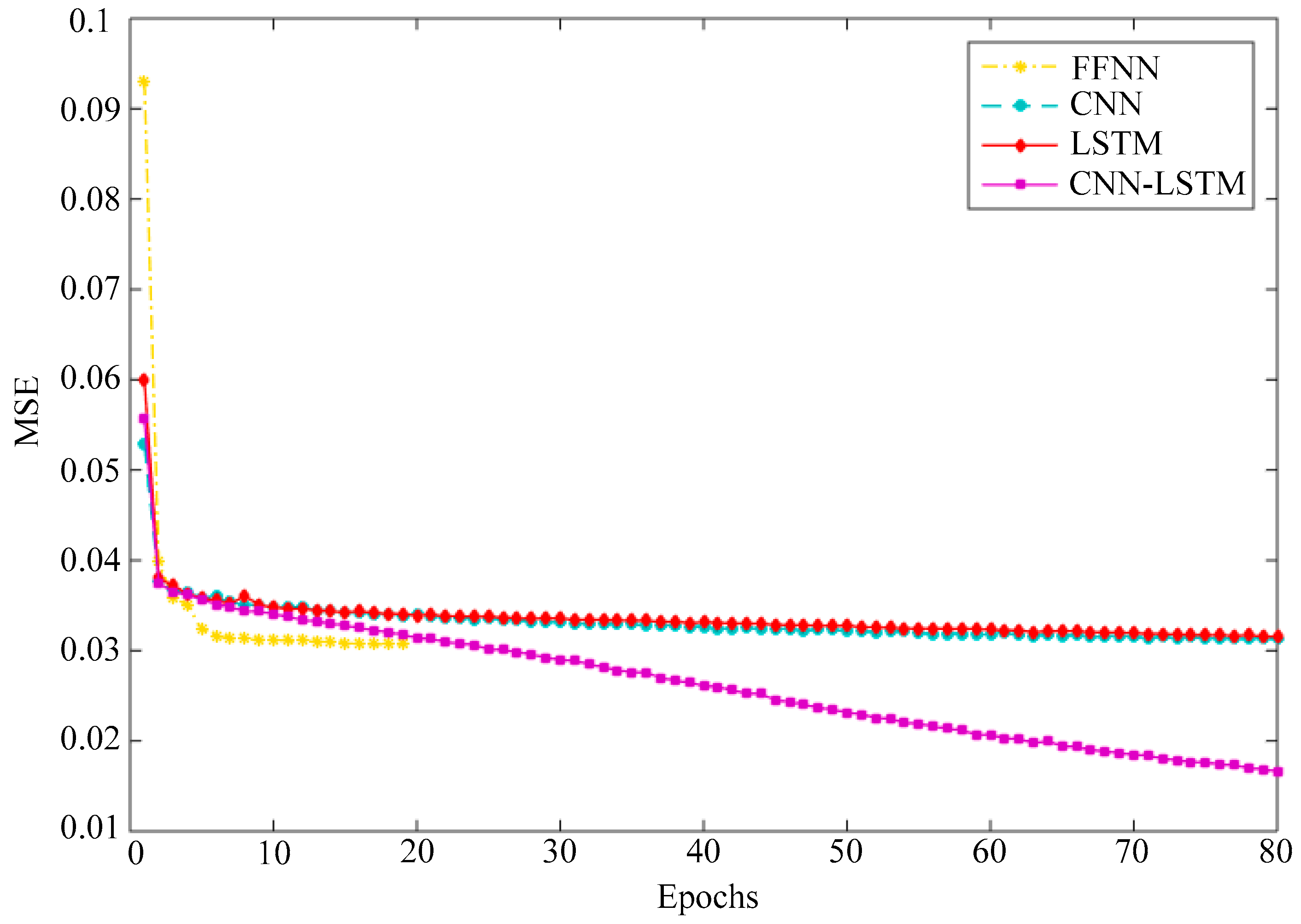
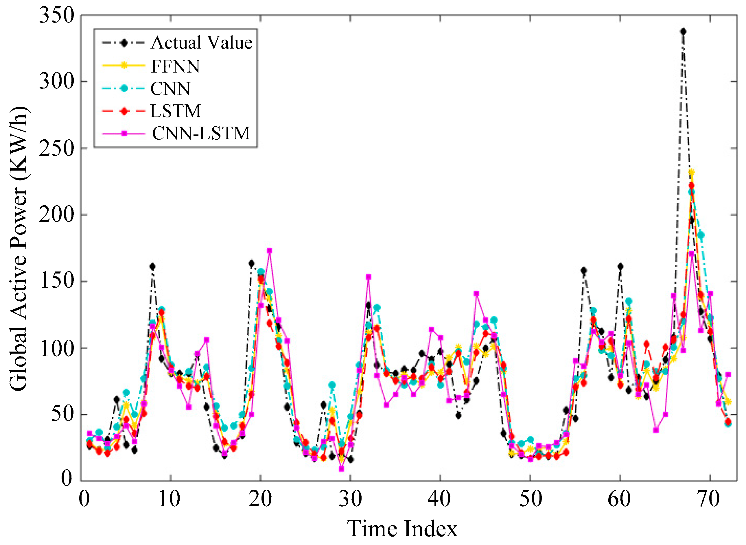
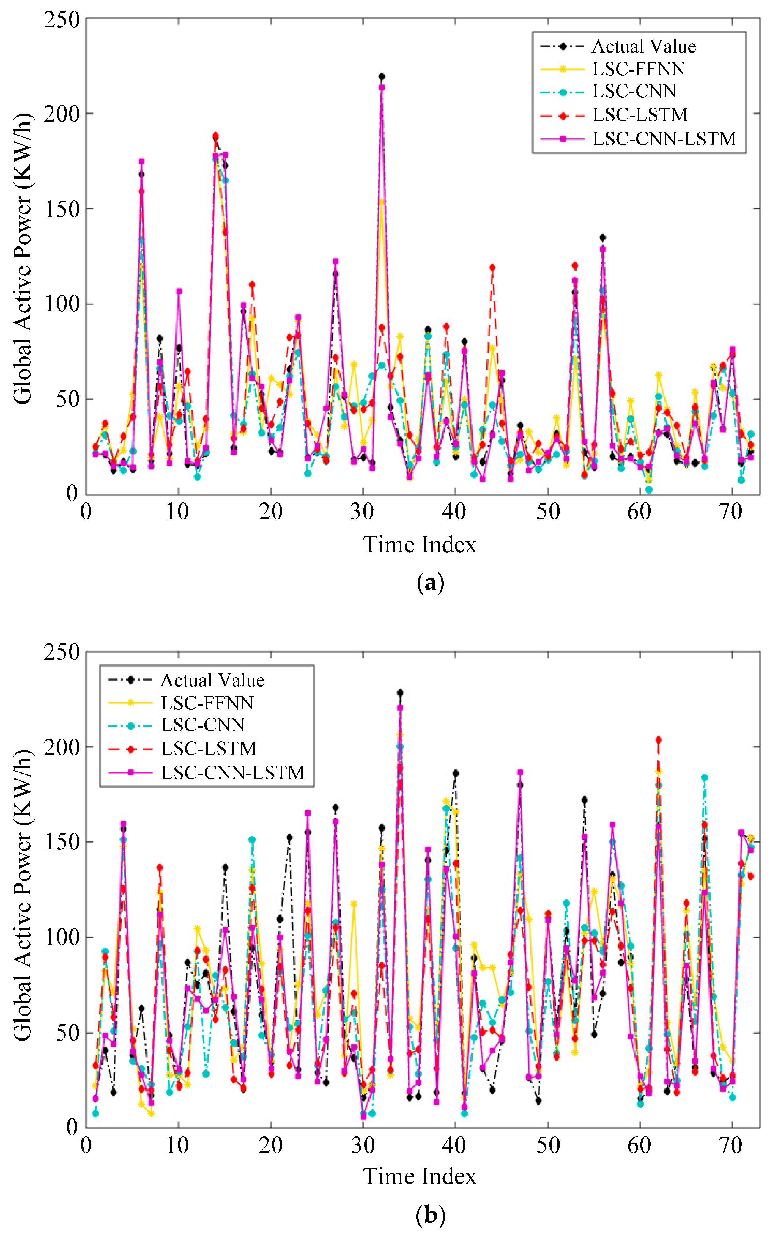
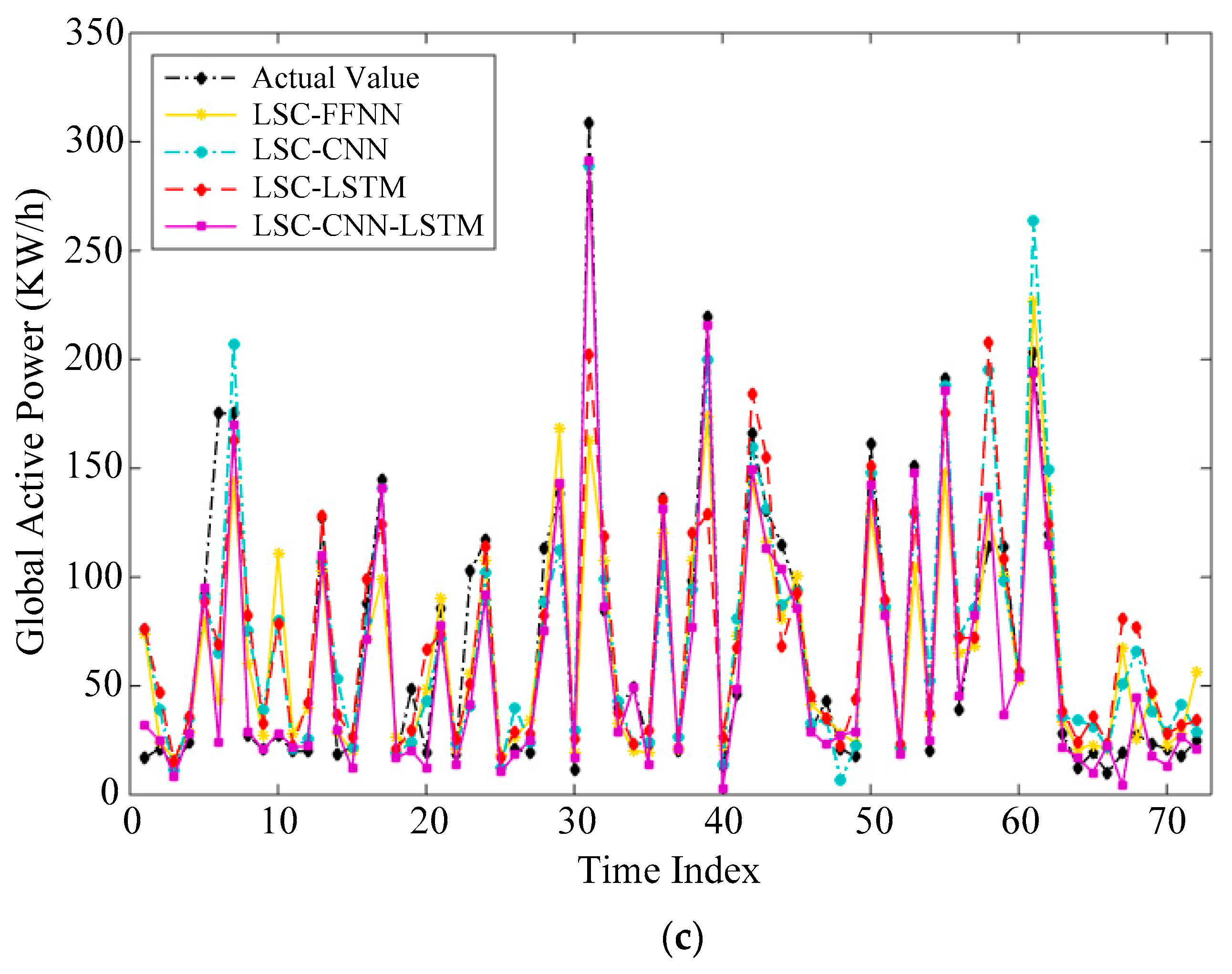
This paper investigates the problem of household electric power prediction. The fluctuation and uncertainty of power consumption bring out great challenges to the prediction of future power consumption. To address these issues, a hybrid forecasting model is proposed by combining LSC, CNN and LSTM. Firstly, the large scale spectral clustering method based on landmarks is employed to cluster all samples according to the periodicity and seasonality of electricity consumption. Then, the samples in each cluster are expanded via the bootstrap aggregating technique. Next, the combined deep learning model is used to accomplish prediction task on all clusters. Finally, the prediction performances of with clustering and without clustering are compared. The experimental results show that the proposed LSC–CNN–LSTM model outperforms other machine learning or deep learning methods in predicting household power consumption. Simultaneously, these results verify the effectiveness of the hybrid deep learning model based on the LSC method and CNN–LSTM.

The combination of clustering and deep learning can effectively deal with the massive samples brought to us in the era of big data and has considerable development prospects in the field of artificial intelligence. This paper only considers one-step prediction and one attribute in household power consumption. Multiple-step prediction involving multiple attributes is quite worthwhile for further research. In addition, although bootstrap aggregating is employed in the proposed method, the ensemble learning technique is not considered. The ensemble of deep learning can yield better generalization performance and provide an interval prediction. Hence, a deep ensemble model will be a promising research subject. All aforementioned models also can be more widely applied in renewable energy fields, such as solar energy, wind energy and geothermal power generation, which is a promising research direction.