
Identifying the Key Driving Factors of Carbon Emissions in ‘Belt and Road Initiative’ Countries

 ,
,
Abstract
:1. Introduction
2. Data and Method
2.1. Data
2.2. The STIRPAT Model
3. Results
3.1. Estimated Coefficients
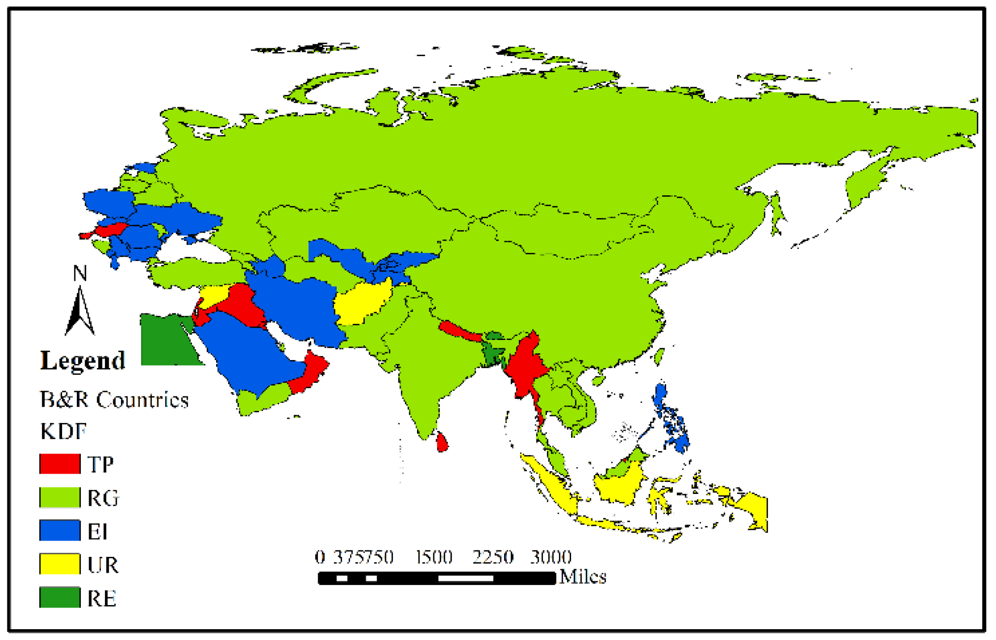
3.2. The KDF in Each B&R Country
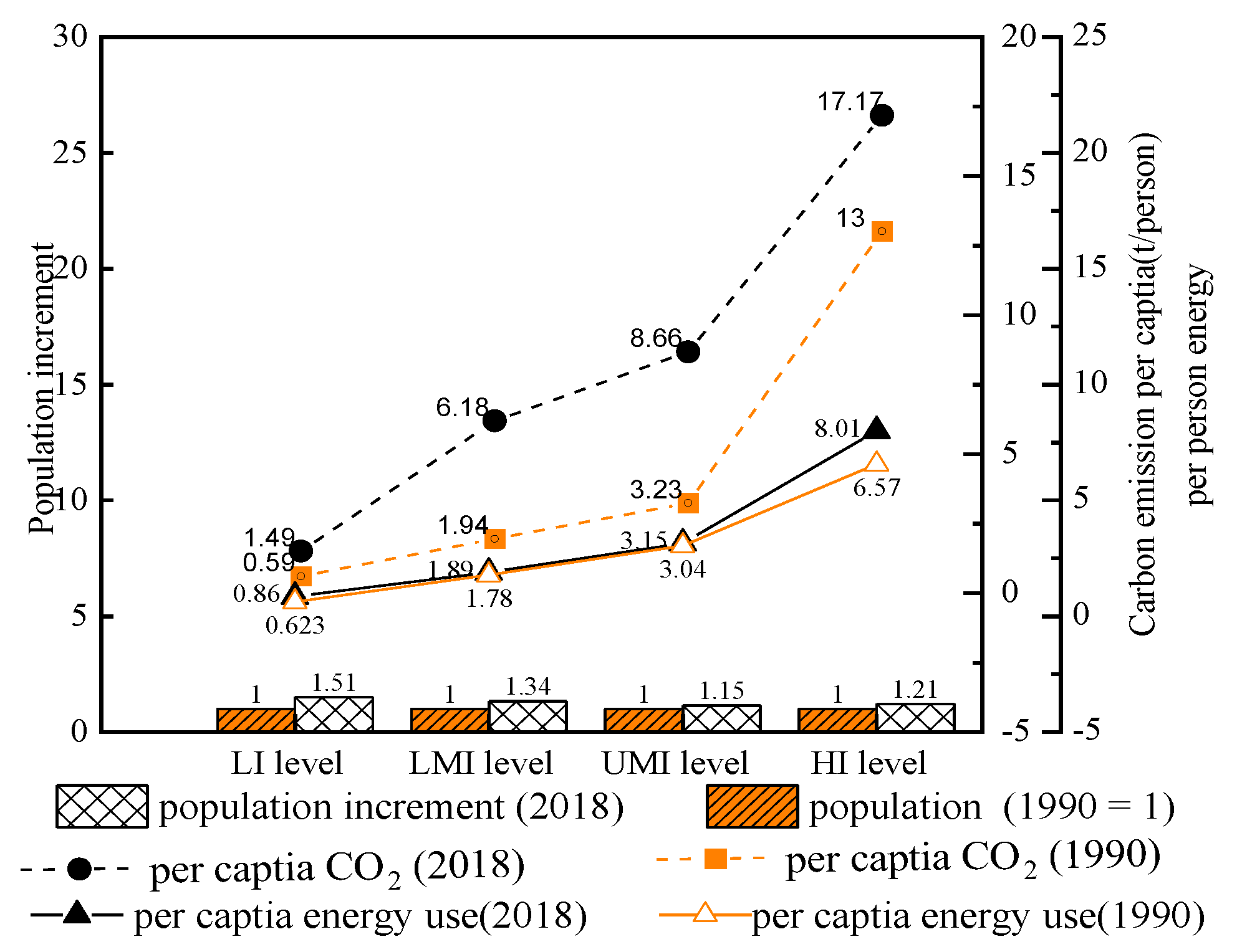
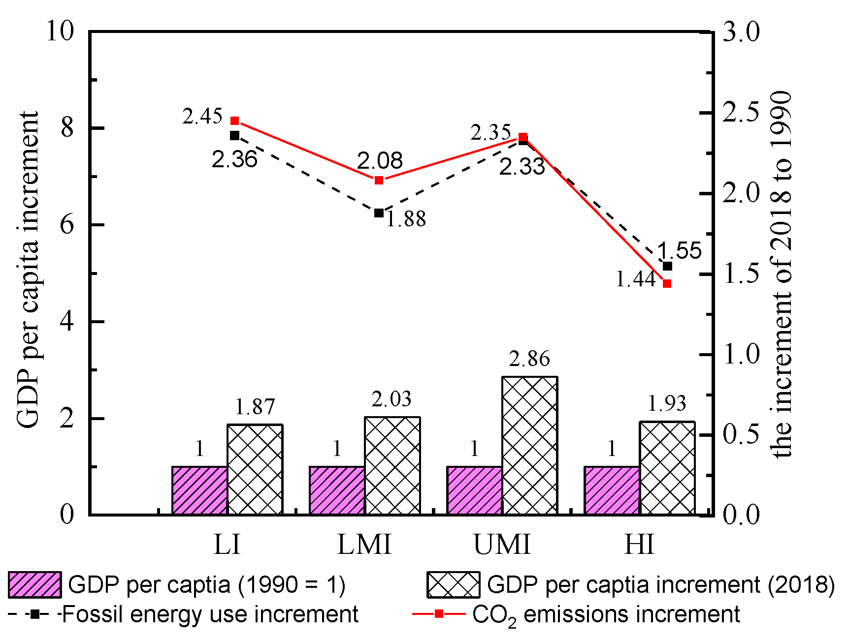
3.3. The KDFs in Different Income Groups
4. Discussion
4.1. Population
4.2. GDP per Capita
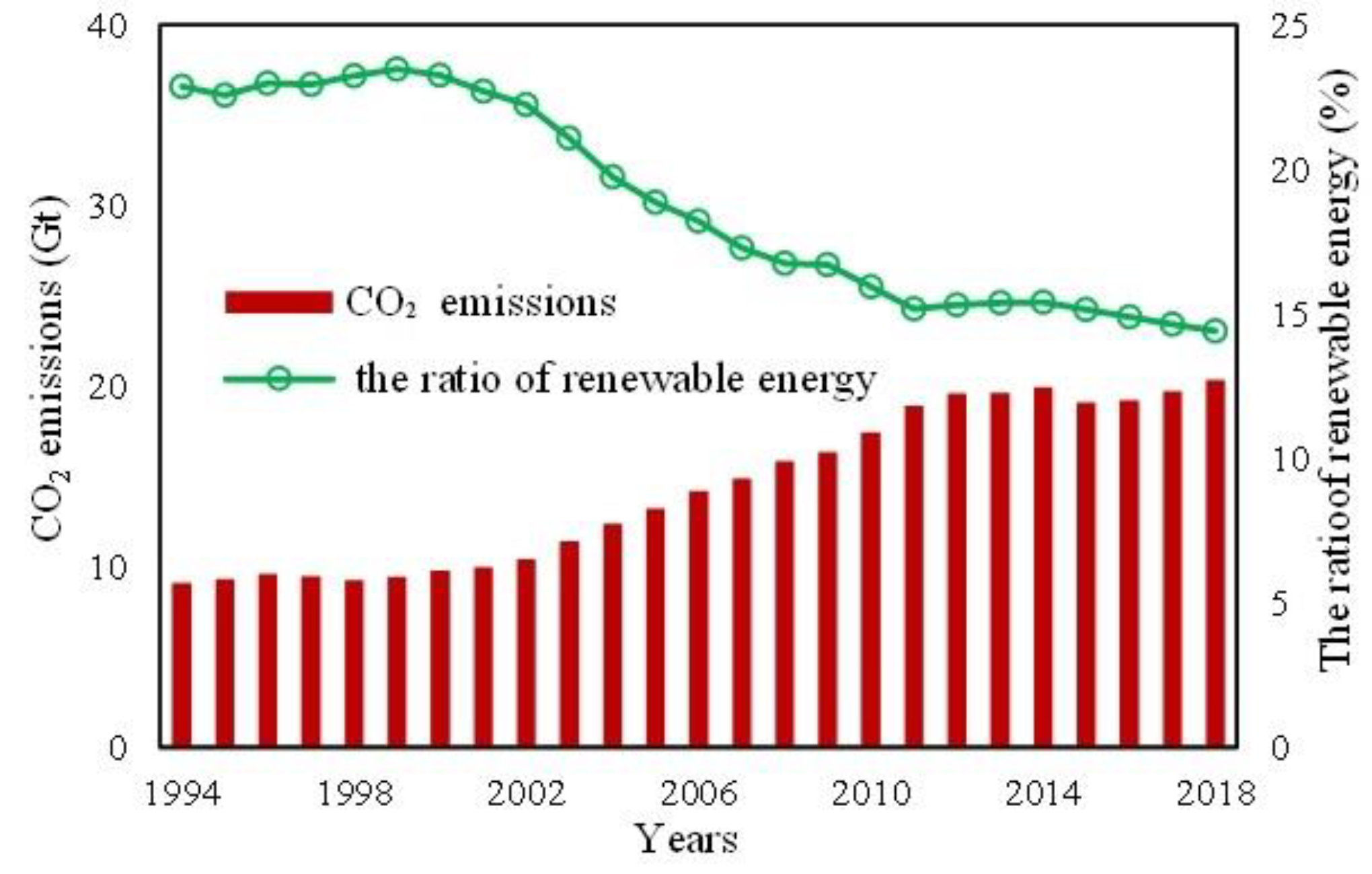
4.3. Energy Intensity
4.4. Urbanization
5. Conclusions and Policy Implications
Author Contributions
Funding
Institutional Review Board Statement
Informed Consent Statement
Data Availability Statement
Conflicts of Interest
Nomenclature
| B&R | Belt and Road Initiative |
| KDFs | key driving factors |
| STIRPAT | Stochastic Impacts by Regression on Population, Affluence, and Technology |
| TP | Total population |
| UR | Urbanization rate |
| RG | GDP per capita FE, RE, IG, RDE, EI, TO, and FDI |
| RDE | Research and development expenditure |
| FDI | Foreign direct investment |
| TO | Trade openness |
| FE | Fossil energy consumption |
| RE | Renewable energy consumption |
| IG | Industry structure |
| EI | Energy intensity |
| HI | High-income level |
| UMI | Upper-middle-income |
| LMI | Low-middle-income |
| LI | Low-income |
Appendix A

| 1 High-income level countries (17 countries with per capita > US$ 12,276 in 2010) |
| Slovenia, Singapore, Saudi Arabia, Qatar, Kuwait, Israel, Brunei, Bahrain, United Arab Emirates, Czech Republic, Hungary, Latvia, Lithuania, Oman, Poland, Slovakia, Estonia |
| 2 Upper-middle-income level groups (16 countries with per capita GNP between US$ 3976 and US$ 12,275 in 2010) |
| Lebanon, Malaysia, Russia, Turkey, Azerbaijani, Belarus, Bulgaria, China, Kazakhstan, Macedonia FTR, Romania, Thailand, Maldives, Serbia, Bosnia and Herzegovina, Montenegro |
| 3 Low-middle-income level groups (19 countries with per capita between US$ 1006 and US$ 3975 in 2010) |
| Albania, Armenia, Georgia, Indonesia, Iran, Iraq, Jordan, Philippines, Sri Lanka, Ukraine, Turkmenistan, Syria Arab Republic, Egypt, India, Moldova, Mongolia, Uzbekistan, Vietnam, Bhutan |
| 4 Low-income level groups (10 countries with per capita GNP < US$ 1005 in 2010) |
| Bangladesh, Cambodia, Kyrgyzstan, Myanmar, Nepal, Pakistan, Tajikistan, Yemen, Afghanistan, Laos |
| Countries | lnC | lnTP | lnUR | lnRG | lnIG | lnFE | lnRE | lnRDE | lnEI | lnTO | LnFDI |
|---|---|---|---|---|---|---|---|---|---|---|---|
| HI group | |||||||||||
| Slovenia | 1 | 0.629 a | −0.795 a | 0.637 a | 0.026 | 0.755 a | −0.271 c | −0.471 | 0.276 b | −0.672 a | 0.002 |
| Singapore | 1 | 0.817 a | - | 0.792 a | −0.039 | −0.166 | −0.128 | −0.581 b | 0.156 b | −0.680 a | −0.288 |
| Saudi Arabia | 1 | 0.904 a | −0.476 b | 0.610 a | 0.402 b | 0.235 | −0.139 | - | 0.832 a | 0.749 a | −0.139 |
| Qatar | 1 | 0.907 a | 0.422 c | 0.936 a | 0.292 c | 0.277 b | −0.038 c | 0.890 a | 0.899 a | 0.540 b | −0.671 a |
| Kuwait | 1 | 0.867 a | −0.792 a | 0.816 a | 0.530 b | 0.458 c | −0.017 | 0.261 c | 0.648 a | −0.448 b | 0.476 c |
| Israel | 1 | 0.927 a | −0.873 a | 0.936 a | 0.430 b | −0.277 | −0.775 a | 0.390 c | 0.857 a | 0.316 | 0.412 |
| Brunei | 1 | 0.605 a | −0.536 a | 0.473 b | 0.400 | 0.273 | −0.640 a | 0.106 | 0.829 a | −0.287 | −0.103 |
| Bahrain | 1 | 0.931 a | −0.837 b | 0.771 a | - | −0.454 b | −0.329 | 0.204 | 0.644 b | −0.139 | −0.109 |
| United Arab Emirates | 1 | 0.621 a | −0.839 a | 0.934 a | 0.502 b | 0.518 b | −0.271 | −0.214 | 0.643 a | 0.743 a | 0.430 b |
| Czech Republic | 1 | −0.712 a | 0.770 a | 0.741 a | −0.358 | 0.889 a | −0.899 a | −0.893 a | 0.764 a | −0.204 | −0.792 a |
| Hungary | 1 | 0.700 a | −0.849 b | 0.420 a | −0.488 b | 0.937 a | −0.933 a | −0.203 | 0.660 a | −0.581 a | 0.087 |
| Latvia | 1 | 0.885 a | 0.635 a | 0.842 a | 0.487 b | 0.603 a | −0.699 a | 0.261 | 0.691 a | −0.201 | 0.371 |
| Lithuania | 1 | 0.589 a | 0.717 a | 0.821 a | −0.745 a | −0.896 a | 0.140 | 0.242 | 0.691 a | −0.501 b | −0.017 |
| Oman | 1 | 0.940 a | 0.683 b | 0.878 a | 0.832 a | 0.194 | 0.152 | −0.139 | 0.914 a | −0.888 a | 0.472 b |
| Poland | 1 | 0.518 a | 0.244 | 0.797 a | −0.669 a | 0.569 a | −0.775 a | 0.500 b | 0.772 a | −0.738 a | −0.431 b |
| Slovakia | 1 | 0.621 b | 0.673 b | 0.910 a | −0.459 b | 0.930 a | −0.490 b | 0.246 | 0.857 a | −0.738 a | −0.103 |
| Estonia | 1 | 0.350 | −0.856 a | 0.730 a | 0.568 b | −0.251 | −0.490 b | 0.012 | 0.548 a | −0.329 | −0.551 a |
| UMI group | |||||||||||
| Lebanon | 1 | 0.842 a | 0.928 b | 0.885 a | 0.294 | 0.749 a | −0.662 b | 0.797 a | 0.246 | −0.699 a | - |
| Malaysia | 1 | 0.771 a | 0.673 b | 0.990 a | 0.633 a | 0.951 a | −0.490 b | 0.106 | 0.229 | −0.078 | −0.368 c |
| Russia | 1 | 0.717 a | −0.573 b | 0.813 a | 0.633 b | 0.724 a | 0.145 | 0.352 c | 0.899 a | −0.873 a | −0.275 |
| Turkey | 1 | 0.684 a | 0.986 a | 0.982 a | −0.639 a | 0.642 b | −0.965 a | −0.551 a | 0.717 a | 0.540 b | 0.525 b |
| Azerbaijani | 1 | 0.737 a | 0.458 b | 0.778 a | −0.214 | 0.547 a | −0.390 c | 0.118 | 0.800 a | 0.418 b | −0.672 a |
| Belarus | 1 | 0.764 a | 0.140 | 0.639 a | −0.169 | 0.071 | 0.145 | 0.012 | 0.718 a | −0.491 b | 0.103 |
| Bulgaria | 1 | 0.717 a | −0.723 a | 0.537 a | 0.672 b | 0.905 a | −0.845 a | 0.576 b | 0.718 a | −0.344 | −0.711 b |
| China | 1 | 0.830 a | 0.974 a | 0.979 a | 0.275 | 0.972 a | −0.994 a | 0.852 a | 0.861 a | −0.738 a | 0.103 |
| Kazakhstan, | 1 | 0.851 a | −0.692 a | 0.715 a | 0.503 b | 0.605 b | −0.724 a | −0.018 | 0.228 | −0.048 | −0.348 |
| Macedonia, FTR | 1 | 0.548 a | 0.624 a | 0.840 a | 0.284 | 0.475 c | −0.857 a | 0.145 | 0.859 a | −0.669 b | 0.012 |
| Romania | 1 | 0.834 a | 0.005 | 0.707 a | 0.672 a | 0.932 a | −0.918 a | 0.810 a | 0.892 a | −0.765 b | −0.652 b |
| Thailand | 1 | 0.976 a | 0.883 a | 0.967 a | 0.282 | 0.879 b | −0.694 a | −0.431 b | 0.878 a | 0.923 a | 0.177 |
| Maldives | 1 | 0.975 a | 0.966 a | 0.622 a | 0.373 | 0.044 | −0.998 a | −0.039 | 0.866 a | 0.486 b | 0.465 b |
| Serbia | 1 | 0.872 a | −0.857 a | 0.642 | −0.919 a | 0.962 a | −0.499 | −0.189 | 0.750 a | −0.763 b | −0.085 |
| Bosnia and Herzegovina | 1 | −0.358 | 0.190 | 0.761 a | −0.092 | 0.882 a | −0.018 | - | 0.619 a | −0.066 | 0.782 a |
| Montenegro | 1 | 0.107 a | 0.901 a | 0.400 a | −0.028 | 0.012 | 0.024 | - | 0.225 a | −0.378 | - |
| LMI group | |||||||||||
| Albania | 1 | −0.611 a | 0.960 a | 0.928 a | 0.546 b | 0.637 a | −0.501 b | 0.104 | 0.838 a | 0.352 | 0.414 b |
| Armenia | 1 | 0.624 a | 0.876 a | 0.944 a | 0.152 | 0.354 | −0.727 a | 0.313 c | 0.691 a | 0.764 a | 0.818 a |
| Georgia | 1 | 0.880 a | −0.886 a | 0.894 a | −0.350 b | 0.916 a | −0.856 a | 0.203 | 0.724 a | 0.022 | −0.293 c |
| Indonesia | 1 | 0.959 a | 0.941 a | 0.950 a | 0.475 b | 0.878 a | −0.931 a | 0.033 | 0.683 a | 0.378 | 0.256 |
| Iran | 1 | 0.993 a | 0.992 b | 0.923 a | 0.666 a | 0.357 | −0.271 | 0.173 | 0.930 a | 0.758 a | 0.409 b |
| Iraq | 1 | 0.901 a | −0.649 a | 0.681 a | −0.149 | −0.672 a | 0.337 | - | 0.501 b | 0.418 b | 0.425 b |
| Jordan | 1 | 0.960 a | 0.899 a | 0.935 a | 0.730 a | 0.200 c | −0.569 a | 0.145 | 0.851 a | −0.105 | 0.676 b |
| Philippines | 1 | 0.936 a | 0.783 a | 0.853 a | −0.444 b | 0.936 a | −0.955 a | 0.044 | 0.743 a | −0.545 b | −0.039 |
| Sri Lanka | 1 | 0.972 a | 0.968 a | 0.946 a | 0.769 a | 0.953 a | −0.952 a | - | 0.811 a | −0.545 a | 0.353 |
| Ukraine | 1 | 0.848 a | 0.758 a | 0.872 a | 0.624 b | 0.921 a | −0.820 a | 0.566 b | 0.750 a | −0.649 b | −0.348 c |
| Turkmenistan | 1 | 0.947 a | 0.973 a | 0.895 a | −0.597 a | 0.145 | 0.336 c | −0.028 | 0.541 a | −0.415 b | 0.450 b |
| Syria Arab Republic | 1 | 0.765 a | 0.875 a | 0.734 a | −0.063 | −0.079 | −0.616 a | −0.075 | 0.372 b | 0.505 a | 0.462 b |
| Egypt | 1 | −0.981 a | 0.828 a | 0.963 a | −0.188 | 0.877 a | −0.947 a | −0.366 c | 0.136 | −0.102 | 0.394 c |
| India | 1 | 0.984 a | 0.994 a | 0.995 a | 0.431 b | 0.985 a | −0.985 a | 0.003 | 0.979 a | 0.961 a | 0.827 a |
| Moldova | 1 | 0.479 b | 0.628 a | 0.734 a | −0.197 | 0.443 c | −0.616 a | 0.254 | 0.529 b | −0.014 | −0.734 a |
| Mongolia | 1 | 0.758 a | 0.791 a | 0.861 a | 0.360 | 0.651 a | −0.297 | −0.366 b | 0.714 a | 0.050 | 0.500 b |
| Uzbekistan | 1 | −0.096 | 0.814 a | 0.654 a | −0.547 a | 0.582 b | −0.484 b | −0.164 | 0.764 a | 0.397 | −0.082 |
| Vietnam | 1 | 0.986 a | 0.984 a | 0.992 a | 0.729 a | 0.991 a | −0.984 a | 0.352 | 0.751 a | 0.355 | −0.819 a |
| Bhutan | 1 | 0.811 a | 0.885 a | 0.893 a | 0.836 a | 0.292 | −0.979 a | 0.246 | 0.857 a | −0.764 a | 0.539 b |
| LI group | |||||||||||
| Bangladesh | 1 | 0.985 a | 0.994 a | 0.987 a | 0.876 a | 0.980 a | −0.996 a | 0.107 | 0.915 a | 0.525 b | −0.849 a |
| Cambodia | 1 | 0.967 a | 0.970 a | 0.976 a | 0.609 b | 0.871 a | −0.944 a | 0.034 | 0.769 a | 0.609 a | 0.651 b |
| Kyrgyzstan | 1 | 0.372 | 0.354 b | 0.712 a | 0.377 c | 0.891 a | 0.208 | −0.085 | 0.819 a | 0.241 | 0.485 b |
| Myanmar | 1 | 0.940 a | 0.922 a | 0.886 a | 0.844 a | 0.880 a | −0.842 a | −0.136 | 0.860 a | 0.448 b | 0.758 a |
| Nepal | 1 | 0.918 a | 0.914 a | 0.921 a | −0.463 c | 0.956 a | −0.942 a | −0.102 | 0.378 | 0.861 a | −0.030 |
| Pakistan | 1 | 0.986 a | 0.987 a | 0.973 a | −0.430 b | 0.939 a | −0.574 b | −0.214 | 0.758 a | −0.515 a | 0.329 |
| Tajikistan | 1 | 0.915 a | 0.754 a | 0.766 a | 0.260 | 0.767 a | −0.527 b | −0.169 | 0.839 a | 0.216 | −0.185 |
| Yemen | 1 | 0.886 a | 0.907 a | 0.973 a | −0.430 b | 0.939 a | −0.474 c | −0.018 | 0.776 a | - | - |
| Afghanistan | 1 | 0.930 a | 0.953 a | 0.975 a | −0.704 b | 0.402 | −0.981 a | - | 0.515 c | 0.529 b | −0.030 |
| Laos | 1 | 0.946 a | 0.950 a | 0.893 a | 0.764 b | 0.230 | 0.747 a | 0.012 | 0.868 a | 0.845 a | 0.255 |
References
- Belt and Road Portal. Belt and Road Report. 2017. Available online: https://www.yidaiyilu.gov.cn/ (accessed on 1 January 2022).
- Han, L.; Han, B.; Shi, X.; Su, B.; Lv, X. Energy efficiency convergence across countries in the context of China’s Belt and Road initiative. Appl. Energy 2018, 213, 112–122. [Google Scholar] [CrossRef] [Green Version]
- Zhang, N.; Liu, Z.; Zheng, X.; Xue, J. Carbon footprint of China’s Belt and Road. Science 2017, 357, 1107. [Google Scholar] [CrossRef]
- World Bank. World Bank Data Indicator (WDI). Available online: https://data.worldbank.org/ (accessed on 1 January 2022).
- Shen, L.; Huang, Y.; Huang, Z.; Lou, Y.; Ye, G.; Wong, S.W. Improved coupling analysis on the coordination between socio-economy and carbon emission. Ecol. Indic. 2018, 94, 357–366. [Google Scholar] [CrossRef]
- De Alegría, I.M.; Basañez, A.; de Basurto, P.D.; Fernández-Sainz, A. Spain’s fulfillment of its kyoto commitments and its fundamental greenhouse gas (ghg) emission reduction drivers. Renew. Sustain. Energy Rev. 2016, 59, 858–867. [Google Scholar] [CrossRef]
- Khan, A.Q.; Saleem, N.; Fatima, S.T. Financial development, income inequality, and CO2emissions in Asian countries using STIRPAT model. Environ. Sci. Pollut. Res. 2018, 25, 6308–6319. [Google Scholar] [CrossRef] [PubMed]
- José, M.; Cansino, R.; Manuel, O. Main drivers of changes in CO2 emissions in the Spanish economy: A structural decomposition analysis. Energy Policy 2016, 89, 150–159. [Google Scholar]
- Diakoulaki, D.; Giannakopoulos, D.; Karellas, S. The driving factors of CO2 emissions from electricity generation in Greece: An index decomposition analysis. Int. J. Glob. Warm. 2017, 13, 382–388. [Google Scholar] [CrossRef]
- Yao, C.; Feng, K.; Hubacek, K. Driving forces of CO2 emissions in the G20 countries: An index decomposition analysis from 1971 to 2010. Ecol. Inf. 2015, 26, 93–100. [Google Scholar] [CrossRef]
- Shuai, C.; Chen, X.; Wu, Y.; Tan, Y.; Zhang, Y.; Shen, L. Identifying the key impact factors of carbon emission in China: Results from a largely expanded pool of potential impact factors. J. Clean. Prod. 2018, 175, 612–623. [Google Scholar] [CrossRef]
- Wang, C.; Wang, F.; Zhang, X.; Yang, Y.; Su, Y.; Ye, Y.; Zhang, H. Examining the driving factors of energy related carbon emissions using the extended STIRPAT model based on IPAT identity in Xinjiang. Renew. Sustain. Energy Rev. 2017, 67, 51–61. [Google Scholar] [CrossRef]
- Xu, B.; Lin, B. Factors affecting carbon dioxide (CO2) emissions in China’s transport sector: A dynamic nonparametric additive regression model. J. Clean. Prod. 2015, 101, 311–322. [Google Scholar] [CrossRef]
- Zhang, C.; Liu, C. The impact of ICT industry on CO2 emissions: A regional analysis in China. Renew. Sustain. Energy Rev. 2015, 44, 12–19. [Google Scholar] [CrossRef]
- Fang, K.; Tang, Y.; Zhang, Q.; Song, J.; Xu, A. Will China peak its energy-related carbon emissions by 2030? lessons from 30 chinese provinces. Appl. Energy 2019, 255, 113852. [Google Scholar] [CrossRef]
- Poumanyvong, P.; Kaneko, S. Does urbanization lead to less energy use and lower CO2 emissions? A cross-country analysis. Ecol. Econ. 2010, 70, 434–444. [Google Scholar] [CrossRef]
- Inmaculada, M.Z.; Antonello, M. The impact of urbanization on CO2 emissions: Evidence from developing countries. Ecol. Econ. 2011, 70, 1344–1353. [Google Scholar]
- Shuai, C.; Shen, L.; Jiao, L.; Wu, Y.; Tan, Y. Identifying key impact factors on carbon emission: Evidences from panel and time-series data of 125 countries from 1990 to 2011. Appl. Energy 2017, 187, 310–325. [Google Scholar] [CrossRef]
- Brizga, J.; Feng, K.; Hubacek, K. Drivers of CO2 emissions in the former soviet union: A country level IPAT analysis from 1990 to 2010. Energy 2013, 59, 743–753. [Google Scholar] [CrossRef]
- Shahbaz, M.; Hye, Q.M.A.; Tiwari, A.K.; Leitão, N.C. Economic growth, energy consumption, financial development, international trade and CO2 emissions in Indonesia. Renew. Sustain. Energy Rev. 2013, 25, 109–121. [Google Scholar] [CrossRef] [Green Version]
- Li, H.; Mu, H.; Zhang, M.; Li, N. Analysis on influence factors of China’s CO2 emissions based on Path–STIRPAT model. Energy Policy 2011, 39, 6906–6911. [Google Scholar] [CrossRef]
- Xiao, B.; Niu, D.; Guo, X. The Driving Forces of Changes in CO2 Emissions in China: A Structural Decomposition Analysis. Energies 2016, 9, 259. [Google Scholar] [CrossRef] [Green Version]
- Fan, Y.; Liuv, L.C.; Wu, G.; Wei, Y.-M. Analyzing impact factors of CO2 emissions using the STIRPAT model. Enviro. Impact Asse. Rev. 2006, 26, 377–395. [Google Scholar] [CrossRef]
- Roula, I.L. Decomposing the South African CO2, emissions within a BRICs countries context: Signalling potential energy rebound effects. Energy 2018, 147, 648–654. [Google Scholar]
- Behera, S.R.; Dash, D.P. The effect of urbanization, energy consumption, and foreign direct investment on the carbon dioxide emission in the ssea (south and southeast asian) region. Renew. Sustain. Energy Rev. 2017, 70, 96–106. [Google Scholar] [CrossRef]
- World Bank. Word band indicator data. Available online: http://data.worldbank.org/indicator (accessed on 1 January 2022).
- Dietz, T.; Rosa, E.A. Rethinking the environmental impacts of population, affluence and technology. Hum. Ecol. Rev. 1994, 1, 277–300. Available online: https://www.jstor.org/stable/24706840 (accessed on 1 January 2022).
- Wang, Y.; Kang, Y.; Wang, J.; Xu, L. Panel estimation for the impacts of population-related factors on CO2 emissions: A regional analysis in China. Ecol. Indic. 2017, 78, 322–330. [Google Scholar] [CrossRef]
- Lu, M. Examining the impact factors of urban residential energy consumption and CO2 emissions in China—Evidence from city-level data. Ecol. Indic. 2017, 73, 29–37. [Google Scholar]
- Wang, Y.N.; Zhao, T. Impacts of energy-related CO2 emissions: Evidence from under developed, developing and highly developed regions in China. Ecol. Indic. 2015, 50, 186–195. [Google Scholar] [CrossRef]
- Abid, M. Does economic, financial and institutional developments matter for environmental quality? a comparative analysis of eu and mea countries. J. Environ. Manag. 2017, 188, 183–194. [Google Scholar] [CrossRef]
- Boutabba, M.A. The impact of financial development, income, energy and trade on carbon emissions: Evidence from the indian economy. Econ. Model. 2014, 40, 33–41. [Google Scholar] [CrossRef] [Green Version]
- Zoundi, Z. CO2 emissions, renewable energy and the environmental kuznets curve, a panel cointegration approach. Renew. Sustain. Energy Rev. 2017, 72, 1067–1075. [Google Scholar] [CrossRef]
- Song, Y.; Zhang, M.; Zhou, Y. Study on the decoupling relationship between CO2 emissions and economic development based on two-dimensional decoupling theory: A case between china and the united states. Ecol. Indic. 2019, 102, 230–236. [Google Scholar] [CrossRef]
- Antonakakisa, N.; Chatziantoniou, I.; Filis, G. Energy consumption, CO2 emissions, and economic growth: An ethical dilemma. Renew. Sustain. Energy Rev. 2017, 68, 808–824. [Google Scholar] [CrossRef] [Green Version]
- Wang, Z.; Yin, F.; Zhang, Y.; Zhang, X. An empirical research on the influencing factors of regional CO2 emissions: Evidence from beijing city, China. Appl. Energy 2012, 100, 277–284. [Google Scholar] [CrossRef]
- Liu, D.; Xiao, B. Can China achieve its carbon emission peaking? a scenario analysis based on stirpat and system dynamics model. Ecol. Indic. 2018, 93, 647–657. [Google Scholar] [CrossRef]
- Zameer, H.; Yasmeen, H.; Zafar, M.W.; Waheed, A.; Sinha, A. Analyzing the association between innovation, economic growth, and environment: Divulging the importance of FDI and trade openness in India. Environ. Sci. Pollut. Res. 2020, 27, 29539–29553. [Google Scholar] [CrossRef]
- Tan, S.; Yang, J.; Yan, J.; Lee, C.; Hashim, H.; Chen, B. A holistic low carbon city indicator framework for sustainable development. Appl. Energy 2017, 185, 1919–1930. [Google Scholar] [CrossRef]
- Dogan, E.; Turkekul, B. CO2 emissions, real output, energy consumption, trade, urbanization and financial development: Testing the EKC hypothesis for the USA. Environ. Sci. Pollut. Res. 2016, 23, 1203–1213. [Google Scholar] [CrossRef]
- Al-Mulali, U.; Tang, C.F.; Ozturk, I. Does financial development reduce environmental degradation? Evidence from a panel study of 129 countries. Environ. Sci. Pollut. Res. 2015, 22, 14891–14900. [Google Scholar] [CrossRef]
- Sharma, S.S. Determinants of carbon dioxide emissions: Empirical evidence from 69 countries. Appl. Energy 2011, 88, 376–382. [Google Scholar] [CrossRef]
- Gullberg, A.T.; Ohlhorst, D.; Schreurs, M. Towards a low carbon energy future—Renewable energy cooperation between Germany and Norway. Renew. Energy 2014, 68, 216–222. [Google Scholar] [CrossRef]
- Shafiei, S.; Salim, R.A. Non-renewable and renewable energy consumption and CO2 emissions in OECD countries: A comparative analysis. Energy Policy 2014, 66, 547–556. [Google Scholar] [CrossRef] [Green Version]
- Balsalobre, L.D.; Shahbaz, M.; Roubaud, D.; Farhanic, S. How economic growth, renewable electricity and natural resources contribute to CO2 emissions? Energy Policy 2018, 113, 356–367. [Google Scholar] [CrossRef] [Green Version]

| Authors | Period | Method | Country | Driving Factor | Result |
|---|---|---|---|---|---|
| Fan et al. (2006) [23] | 1975–2000 | STIRPAT | 208 countries | TP RG EI UR WP | TP→+CO2 (KDF in UMI group) RG→+CO2 (KDF in LMI group) WP→−CO2 (in HI group) WP→+CO2 (in LMI and LI group) UR→+CO2 (KDF in LI group) EI→−CO2 |
| Poumanyvong and Kaneko (2010) [16] | 1975–2005 | STIRPAT | 99 countries | TP UR RG EI IG EC | UR→+CO2 UR→−EI (LI group) UR→+EI (MI and HI group) |
| Brizga et al. (2013) [19] | 1990–2010 | IDA | Former soviet union | TP RG FE IG EI | RG→+CO2 (KDF in 1971–1990, 2001–2010) EI→+CO2 (KDF in 1991–2000) TP→+CO2 (2001–2005) FE→+CO2 (2001–2005) TP &FE→×CO2 (2006–2010) |
| Khan et al.(2018) [7] | 1980–2014 | STIRPAT | Three developing Asian countries | RG FD income inequality EI | EC→+CO2 (KDF) FD→+CO2 financial development Income inequality→+CO2 (Bangladesh) Income inequality→−CO2 (Pakistan and India) |
| Inmaculada et al. (2011) [17] | 1975–2003 | STIRPAT | 93 developing countries | TP RG EI UR WP | TP→+CO2 RG→+ CO2 (KDF in the short term) EI→−CO2 UR→+CO2 (LI group) UR→−CO2 (MI and HI group) |
| Yao et al. (2015) [10] | 1971–2010 | IDA | G20 countries | RG TP IG EI | RG→+CO2 (KDF in China, India, Australia, and Korea) TP→+CO2 (KDF in South Africa, Brazil, Mexico, Argentina, and Turkey) EI→+CO2 (KDF in Saudi Arabia) IG→−CO2 (Saudi Arabia, South Africa, Argentina, Australia) |
| Shuai et al. (2017b) [18] | 1990–2011 | IPAT | 125 countries | RG UR EI | RG→+CO2 (KDF for UMI, LMI, LI) EI→+CO2 (KDF for HI) UR→+CO2 |
| Irziar et al. (2016) [6] | 2005–2012 | STIRPAT | Spain | RG RE EI TP | RG→+CO2 (KDF) RE→−CO2 EI→+CO2 TP→+CO2 |
| Shahbaz et al.(2013) [20] | 1975–2011 | STIRPAT | Indonesia | RG EI TO FD | EI→+CO2 (KDF) RG→+CO2 FD→+CO2 TO→+CO2 |
| Roula Inglesi-Lotz (2018) [24] | 1990–2014 | IDA | South African and BRICS countries | TP EI RG IG | RG→+CO2 (KDFs in Brazil, China, India) TP→+CO2 (KDFs in South Africa) IG→+CO2 (KDFs in Russia) |
| Behera & Dash (2017) [25] | 1980–2012 | STIRPAT | SSEA(South and Southeast Asian | UR FE EC FDI | FE, EC, FDI→+CO2 (in HI and MI group) FE, EC→+CO2 (in LI group) ER, FDI→×CO2 (in LI group) |
| Li et al. (2011) [21] | 1991–2009 | STIRPAT | China | TP RG EI UR | TP→+CO2 RG→+CO2 (KDF) UR→+CO2 EI→+CO2 |
| José M.Cansino (2016) [8] | 1995–2005 | SDA | Spain | ES EI, FDE SE | SE→CO2 (KDF) ES (FE↓, RE↑)→−CO2 EI→−CO2 Policy→FDE |
| Xiao et al. (2016) [22] | 1997–2010 | SDA | China | ES EI, FDE | EI→−CO2 ES (FE↓, RE↑)→−CO2 FDE→+CO2 (KDF) |
| Variable | Short Name | Description | Unit |
|---|---|---|---|
| C | Carbon emissions | Carbon emissions from energy-relate | Kt |
| TP | population | total population | Ten thousand person |
| UR | Urbanization | The ratio of urban population to total population | % |
| RG | GDP per capita | Real GDP per capita | % |
| RDE | Research and development expenditure | The ratio of the Research and development expenditure over the total GDP | % of GDP |
| FDI | foreign direct investment | The ratio of total foreign direct investment in GDP | % of GDP |
| TO | Trade openness | The total export and import goods and services in GDP | % of GDP |
| FE | fossil energy consumption | The ratio of fossil energy in total energy consumption | % |
| RE | renewable energy consumption | The ratio of renewable energy in total energy consumption | % |
| IG | Industry structure | The industrial value-added over the total GDP | constant 2011 US (% of GDP) |
| EI | Energy intensity | Energy consumption per GDP | kg of oil equivalent per constant 2010 PPP$ |
| Countries | Optimal STIRPAT Model | R2 | Residual |
|---|---|---|---|
| HI level | |||
| Slovenia | lnC = 10.282 a + 0.811 a lnTP − 0.753 a LnUR + 0.69 a lnRG + 0.171 a lnFE − 0.48 a lnTO | 0.887 | 0.0263 |
| Singapore | lnC = 10.684 b + 0.63 a lnTP − 0.475 a lnRG − 0.121 b lnTO | 0.82 | 0.07197 |
| Saudi Arabia | lnC = 12.739 a + 0.068 b lnTP + 0.107 a lnRG + 0.229 a lnEI + 0.109 a lnTO | 0.967 | 0.09436 |
| Qatar | lnC = 10.828 b + 0.067 a lnTP + 0.098 a lnRG + 0.096 a lnEI − 0.015 a lnFDI | 0.989 | 0.0132 |
| Kuwait | lnC = 10.641 b + 0.374 a lnTP − 0.314 a lnUR + 0.219 a lnRG + 0.151 a lnEI | 0.994 | 0.0225 |
| Israel | lnC = 10.713 a + 0.475 a lnTP − 0.414 a lnUR + 0.22 a lnRG − 0.013 a lnRE + 0.119 a lnEI | 0.992 | 0.01939 |
| Brunei | lnC = 8.678 a + 0.234 a lnTP − 0.354 a lnUR + 0.377 a lnEI | 0.933 | 0.1122 |
| Bahrain | lnC = 9.744 a + 0.266 a lnTP − 0.085 b lnUR + 0.037 b lnRG + 0.055 b lnEI | 0.889 | 0.11917 |
| United Arab Emirates | lnC = 11.496 b − 0.010 a lnUR + 0.44 a lnRG + 0.479 a lnEI | 0.937 | 0.17732 |
| Czech Republic | lnC = 11.676 a − 0.038 a lnUR + 0.168 a lnRG + 0.088 a lnFE + 0.012 a lnEI − 0.012 a lnFDI | 0.973 | 0.01783 |
| Hungary | lnC = 10.399 b + 0.359 a lnTP + 0.097 a lnRG + 0.101 a lnFE + 0.131 a lnEI | 0.987 | 0.01687 |
| Latvia | lnC = 8.189 a + 0.047 a lnTP + 0.024 b lnUR + 0.412 a lnRG − 0.036 a lnRE + 0.371 a lnEI | 0.99 | 0.01178 |
| Lithuania | lnC = 8.971 b + 0.132 a lnTP − 0.033 a lnUR + 0.327 a lnRG + 0.107 a lnFE + 0.284 a lnEI | 0.967 | 0.01873 |
| Oman | lnC = 10.164 a + 0.33 a lnTP + 0.127 a lnRG + 0.256 a lnEI − 0.097 a lnTO | 0.966 | 0.1148 |
| Poland | lnC = 12.198 a + 0.009 a lnTP + 0.227 a lnRG + 0.019 a lnFE + 0.245 a lnEI | 0.995 | 0.00451 |
| Slovakia | lnC = 9.846 b + 0.199 a lnRG + 0.065 a lnFE + 0.235 a lnEI + 0.017 a lnTO | 0.973 | 0.01538 |
| Estonia | lnC = 4.914 a − 0.022 a lnUR + 0.005 a lnRG + 0.05 a lnEI | 0.983 | 0.00362 |
| UMI level | |||
| Lebanon | lnC = 9.650 a + 0.158 a lnTP + 0.093 a lnRG + 0.06 a lnFE − 0.058 b lnTO | 0.951 | 0.06774 |
| Malaysia | lnC = 11.85 a + 0.293 a lnRG + 0.108 a lnFE − 0.022 b lnGI | 0.993 | 0.05212 |
| Russia | lnC = 13.892 a + 0.049 a lnTP − 0.019 a lnUR + 0.3 ln a RG + 0.216 a lnEI − 0.004 b lnTO | 0.995 | 0.00658 |
| Turkey | lnC = 12.208 a + 0.082 b lnUR + 0.209 a lnRG − 0.024 a lnRE + 0.051 b lnEI − 0.004 b lnIG | 0.999 | 0.00864 |
| Azerbaijani | lnC = 10.437 a + 0.696 a lnRG + 0.699 a lnEI − 0.018 b lnFDI | 0.947 | 0.0419 |
| Belarus | lnC = 11.023 a + 0.232 a lnTP + 0.499 a lnRG + 0.271 a lnEI − 0.024 b lnTO | 0.938 | 0.0313 |
| Bulgaria | lnC = 10.816 a + 0.227 a lnRG + 0.077 a lnFE + 0.270 a lnEI | 0.959 | 0.032 |
| China | lnC = 14.743 a + 0.786 a lnRG − 0.027 b lnRE + 0.320 a lnEI − 0.01 b lnTO | 0.998 | 0.02014 |
| Kazakhstan, | lnC = 12.11 a + 0.213 a lnTP − 0.644 a lnUR + 0.71 a lnRG − 0.051 a lnRE | 0.979 | 0.04586 |
| Macedonia, FTR | lnC = 9.239 a + 0.115 a lnTP + 0.37 a lnRG − 0.058 a lnRE + 0.534 b lnEI | 0.964 | 0.05432 |
| Romania | lnC = 11.52 a + 0.053 a lnTP + 0.272 a lnRG + 0.101 a lnFE +0.298 a lnEI | 0.998 | 0.01045 |
| Thailand | lnC = 12.19 a + 0.106 a lnTP + 0.038 b lnUR + 0.234 a lnRG − 0.056 b lnRE + 0.045 a lnEI − 0.02 b lnTO | 0.997 | 0.0213 |
| Maldives | lnC = 6.413 a + 0.177 a lnTP + 0.13 b lnUR + 0.093 a lnRG − 0.093 b lnRE + 0.069 b lnEI | 0.999 | 0.01506 |
| Serbia | lnC = 10.651 a + 0.121 a lnTP − 0.013 b lnIG + 0.054 a lnFE + 0.06 a lnEI | 0.996 | 0.0068 |
| Bosnia and Herzegovina | lnC = 9.082 a + 0.47 a lnRG + 0.197 a lnFE + 0.136 a lnEI + 0.014 b lnFDI | 0.999 | 0.01093 |
| Montenegro | lnC = 7.744 a + 0.071 b lnUR + 0.105 a lnRG + 0.205 a lnEI − 0.059 b lnTO | 0.984 | 0.02048 |
| LMI level | |||
| Albania | lnC = 7.132 a + 0.306 a lnUR + 0.411 a lnRG + 0.51 a lnEI | 0.945 | 0.09761 |
| Armenia | lnC = 7.955 a + 0.374 a lnUR + 0.654 a lnRG − 0.11 a lnRE + 0.166 a lnEI + 0.15 a lnTO + 0.147 a lnFDI | 0.97 | 0.05471 |
| Georgia | lnC = 8.628 a − 0.249 a lnUR + 0.747 a lnRG − 0.206 a lnRE + 0.511 a lnEI | 0.955 | 0.0233 |
| Indonesia | lnC = 12.64 a + 0.847 a lnUR + 0.231 b lnRE − 0.097 a lnEI + 0.066 a lnTO + 0.322 b lnRG | 0.949 | 0.09458 |
| Iran | lnC = 12.872 a + 0.253 a lnTP + 0.046 a lnRG + 0.066 a lnEI + 0.017 a lnTO | 0.99 | 0.04029 |
| Iraq | lnC = 11.107 a + 0.357 a lnTP + 0.043 b lnUR + 0.099 a lnRG − 0.062 b lnRE + 0.526 a lnEI | 0.895 | 0.06551 |
| Jordan | lnC = 9.619 a + 0.246 a lnTP + 0.103 a lnRG − 0.032 a lnRE + 0.061 a lnEI | 0.99 | 0.02983 |
| Philippines | lnC = 10.61 a + 0.209 a lnTP + 0.196 a lnRG − 0.072 a lnFE + 0.266 a lnEI − 0.032 b lnTO | 0.99 | 0.02666 |
| Sri Lanka | lnC = 8.771 b + 0.322 a lnTP + 0.191 a lnRG − 0.101 a lnRE + 0.187 a lnEI | 0.99 | 0.04897 |
| Ukraine | lnC = 12.211 a + 0.11 a lnTP + 0.103 a lnUR + 0.216 a lnRG + 0.123 a lnFE + 0.226 a lnEI | 0.988 | 0.02896 |
| Turkmenistan | lnC = 10.321 a + 0.099 a lnUR + 0.326 a lnRG − 0.024 b lnIG + 0.184 a lnEI | 0.998 | 0.01199 |
| Syria Arab Pepublic | lnC = 10.776 a + 0.084 a lnTP + 0.126 a lnUR − 0.058 b lnRE | 0.868 | 0.08974 |
| Egypt | lnC = 11.833 a + 0.049 a lnUR + 0.148 a lnRG − 0.208 a lnRE | 0.976 | 0.0596 |
| India | lnC = 13.564 a + 0.136 a lnUR + 0.317 a lnRG + 0.103 a lnFE + 0.19 a lnEI + 0.016 a lnFDI | 0.998 | 0.01731 |
| Moldova | lnC = 8.554 a + 0.315 a lnUR + 0.344 a lnRG − 0.125 a lnRE − 0.11 b lnFDI | 0.951 | 0.03236 |
| Mongolia | lnC = 9.174 a +0.253 a lnRG + 0.154 b lnFE + 0.004 a lnEI | 0.897 | 0.05987 |
| Uzbekistan | lnC = 9.043 a + 0.077 a lnUR + 0.29 a lnRG + 0.315 a lnFE − 0.045 a lnRE + 1.32 a lnEI | 0.934 | 0.02114 |
| Vietnam | lnC = 11.059 a + 0.664 a lnUR + 1.088 a lnRG − 0.283 a lnRE−0.067 b lnFDI | 0.997 | 0.01433 |
| Bhutan | lnC = 5.917 a + 0.037 b lnRG − 0.42 a lnRE + 0.068 a lnTO | 0.98 | 0.07517 |
| LI level | |||
| Bangladesh | lnC = 10.419 a + 0.216 a lnTP + 0.031 b lnRG − 0.289 a lnRE − 0.046 b lnFDI | 0.998 | 0.02146 |
| Cambodia | lnC = 7.344 a + 0.539 a lnRG + 0.231 a lnFE + 0.321 a lnEI | 0.995 | 0.03316 |
| Kyrgyzstan | lnC = 8.344 a + 0.133 a lnRG + 0.09 a lnFE + 0.215 a lnEI + 0.014 b lnFDI | 0.988 | 0.03076 |
| Myanmar | lnC = 8.771 a + 0.473 a lnTP − 0.093 a lnRE + 0.173 b lnEI | 0.938 | 0.05651 |
| Nepal | lnC = 7.952 a + 1.135 b lnTP + 0.237 a lnUR + 0.397 a lnRG +0.287 a lnFE + 0.073 a lnTO | 0.986 | 0.01761 |
| Pakistan | lnC = 11.492 a + 0.164 a lnTP + 0.213 a lnRG + 0.084 a lnEI | 0.995 | 0.02122 |
| Tajikistan | lnC = 7.94 a + 0.622 a lnTP + 0.128 b lnUR + 0.499 a lnRG + 0.908 a lnEI | 0.938 | 0.02081 |
| Yemen | lnC = 11.492 a + 0.342 a lnRG + 0.032 b lnFE + 0.083 a lnEI | 0.979 | 0.04076 |
| Afghanistan | lnC = 8.196 a + 0.16 b lnRG + 0.283 a lnUR − 0.191 a lnRE | 0.998 | 0.05743 |
| Laos | lnC = 6.672 a + 0.73 a lnTP + 1.954 a lnRG + 0.392 a lnRE + 0.655 a lnEI | 0.984 | 0.01191 |
| B&R Countries | TP | RG | EI | UR | RE |
|---|---|---|---|---|---|
| HI | |||||
| Number of countries with KDF (percentage) | 7 (41%) | 4 (24%) | 6 (35%) | ||
| Coefficient (median) | 0.374 | 0.262 | 0.351 | ||
| UMI | |||||
| Number of countries with KDF (percentage) | 3 (19%) | 8 (50%) | 5 (31%) | ||
| Coefficient (median) | 0.158 | 0.346 | 0.27 | ||
| LMI | |||||
| Number of countries with KDF (percentage) | 3 (16%) | 7 (37%) | 5 (26%) | 2 (11%) | 2 (11%) |
| Coefficient (median) | 0.322 | 0.353 | 0.266 | 0.236 | −0.372 |
| LI | |||||
| Number of countries with KDF (percentage) | 2 (20%) | 4 (40%) | 2 (20%) | 1 (10%) | 1 (10%) |
| Coefficient (median) | 0.352 | 0.369 | 0.235 | 0.183 | −0.289 |
Publisher’s Note: MDPI stays neutral with regard to jurisdictional claims in published maps and institutional affiliations. |
© 2022 by the authors. Licensee MDPI, Basel, Switzerland. This article is an open access article distributed under the terms and conditions of the Creative Commons Attribution (CC BY) license (https://creativecommons.org/licenses/by/4.0/).
Share and Cite
Sun, L.; Yu, H.; Liu, Q.; Li, Y.; Li, L.; Dong, H.; Adenutsi, C.D. Identifying the Key Driving Factors of Carbon Emissions in ‘Belt and Road Initiative’ Countries. Sustainability 2022, 14, 9104. https://doi.org/10.3390/su14159104
Sun L, Yu H, Liu Q, Li Y, Li L, Dong H, Adenutsi CD. Identifying the Key Driving Factors of Carbon Emissions in ‘Belt and Road Initiative’ Countries. Sustainability. 2022; 14(15):9104. https://doi.org/10.3390/su14159104
Chicago/Turabian StyleSun, Lili, Hang Yu, Qiang Liu, Yanzun Li, Lintao Li, Hua Dong, and Caspar Daniel Adenutsi. 2022. "Identifying the Key Driving Factors of Carbon Emissions in ‘Belt and Road Initiative’ Countries" Sustainability 14, no. 15: 9104. https://doi.org/10.3390/su14159104
APA StyleSun, L., Yu, H., Liu, Q., Li, Y., Li, L., Dong, H., & Adenutsi, C. D. (2022). Identifying the Key Driving Factors of Carbon Emissions in ‘Belt and Road Initiative’ Countries. Sustainability, 14(15), 9104. https://doi.org/10.3390/su14159104