An Assessment of the Impact of Temperature Rise Due to Climate Change on Asphalt Pavement in China

Abstract

In the global warming context, understanding the impact of temperature rise on asphalt pavement is the basis for making adaptation strategies. An approach based on historical climate data and pavement performance models was employed to assess the potential impact of temperature rise on asphalt pavement in China. It is shown that permanent deformation is one sensitive aspect of asphalt pavement performance, which increased on average by 20.70% from 1992 to 2019. Another one is low-temperature cracking, which decreased by 20.99% from 1970 to 1997, but has remained almost unchanged since 1997. Global mean surface temperature anomalies of 1.5 °C and 2.0 °C will increase the permanent deformation of asphalt pavement by 18.63% and 36.71%, respectively, compared to 2019. Global warming is bringing serious challenges to the structure and material design of asphalt pavement due to the increasing service temperature range.

1. Introduction

There is a lot of evidence showing that the climate is changing at an alarming rate [1]. The rising global mean surface temperature (GMST) is one of the typical features of climate change according to the sixth assessment report of the Intergovernmental Panel on Climate Change (IPCC) [2]. The performance of asphalt pavement depends on the temperature of its service environment since asphalt binder is temperature sensitive. It is necessary to quantitatively assess the potential effects of temperature rise due to climate change on asphalt pavement, which helps understand what the temperature rise means exactly for asphalt pavement and developing adaptation strategies. The assessment mainly involves two issues: (1) climatic conditions and their future changes, and (2) prediction of asphalt pavement performance under given climatic conditions.

In past decades, many models have been proposed to simulate future global or regional climate [3,4,5,6,7,8]. The projections of these models provide data support for assessing the potential effects of climate change on asphalt pavement. However, the spatial and temporal resolutions of these projections and the included indicators usually could not directly meet the requirements of asphalt pavement performance evaluation [8]. A lot of research focuses on bridging these gaps. Austroads [9,10] developed a climate tool according to the needs of the pavement performance prediction model, which includes the historical and simulated climate data of Australia between 1960 and 2099. The simulated climate data were developed based on the projections of the atmosphere-ocean global climate model (AOGCM) and the conformal-cubic general circulation model (GCM) proposed by the Commonwealth Scientific and Industrial Research Organisation (CSIRO). Many researchers also obtained local climate data to assess asphalt pavement performance by downscaling the projections of global or regional climate models [11,12,13,14]. Since the projections of different climate models are significantly different from each other, incorporating multiple models is a common strategy to improve the assessment reliability [15,16,17,18]. The Coupled Model Intercomparison Project (CMIP) has brought much convenience for doing that [3].

Greenhouse gas (GHG) emissions are considered the major contributor to climate change. In 2000, the IPCC [19] released a special report on emissions scenarios (SRES), in which a series of future scenarios was described and the potential GHG emissions corresponding to each scenario were predicted. In 2007, the IPCC [20] released the Representative Concentration Pathways (RCPs) to replace the SRES scenarios. The SRES scenarios and RCPs have been the most frequently referenced emission-level systems in the assessment of climate change on asphalt pavement [21,22,23,24].

Though the projections of climate models provide a foundation for quantitatively assessing the impact of climate change on asphalt pavement, there are also some problems that are difficult to deal with. The first is the mismatch of spatial and temporal resolutions between projections and needs. Downscaling the projections is one approach to make up for the mismatch, but it is at the expense of reliability, which increases the uncertainty of the assessment based on the projections. The second is the differences in projections between various climate models. It is difficult to find an objective basis for processing and screening the projections derived from various models. The historical observational climate data imply rich information, which have important reference value for asphalt pavement, whose life cycle is about 10 to 20 years. In the research based on the projections of climate models, the historical climate data were usually used as baselines only. The implied information has not been well mined and utilized. Viola and Celauro [25] investigated the effects of climate change on asphalt binder selection based on the observational climate data of Italy from 1984 to 2013. They employed the non-parametric Mann-Kendall test to detect the trend of considered climate indicators and extrapolated their values in 2033. However, work based on historical climate data is still rarely reported.

Pavement performance prediction is one of the most important tasks in pavement design and management. Many methods and models have been proposed for asphalt pavement performance prediction, and most of them take the influence of climatic conditions into account. They provide good options for evaluating the performance of asphalt pavement under projected future climatic conditions. The mechanistic empirical pavement design guide (MEPDG), released by the American Association of State Highway and Transportation Officials (AASHTO), are often used with the AASHTOWare Pavement ME software tool in assessing the potential effects of climate change [26,27,28,29]. Many other design methods and tools, such as CHAUSSEE 2 [30], MnPAVE [12], and mePADS [31], are also employed. The models and tools for pavement management are also widely applied to assess the effects of climate change. Among them, the highway development and management tool version 3 and version 4 (HDM-3 and HDM-4) are the most commonly used [11,32]. Moreover, field inspection, laboratory tests, and numerical simulation are commonly used methods to evaluate pavement performance [33]. Based on these or existing knowledge, many researchers have constructed models with regression analysis [34], artificial neural networks (ANN) [34,35], fuzzy inferences [36], systems dynamics [18,37], etc. The life cycle cost analysis (LCCA) and risk assessment (RA) are often incorporated in the assessment to quantify the potential loss and risk [17,23,38,39].

Previous studies provide many perspectives for understanding the potential effects of climate change on asphalt pavement. However, most of them were performed based on the projections of climate models. It is necessary to explore the potential impact with the information implied in historical climate data. This will not only enhance the understanding of possible future impacts, but also enrich the toolbox for dealing with such issues.

The objective of this paper is to quantitatively assess the impact of climate change on asphalt pavement in China at a macro (national) level to support adaptation policy formulation. An assessment was carried out using the meteorological data of 699 meteorological stations around China from 1961 to 2019 and the prediction models of asphalt pavement performance in the Specifications for Design of Highway Asphalt Pavement (JTG D50-2017) of China [40]. Firstly, the temperature-related parameters for asphalt pavement performance prediction were calculated year by year from 1970 to 2019. The changes in these parameters were employed to quantify the impact on asphalt pavement in the past. Then, the relationships between those parameters and the GMST anomaly were established using the regression method, based on which the potential impact of global warming of 1.5 °C and 2.0 °C on asphalt pavement in China was quantitatively assessed.

2. Temperature-Related Parameters for Asphalt Pavement Performance Prediction

The impact of temperature conditions was systematically considered in JTG D50-2017 [40]. Three temperature calibration coefficients were defined for characterizing the impact of temperature conditions on the fatigue lives of asphalt layers (FLAL) and inorganic binder stabilized layers (FLIBSL), and the allowable vertical compressive strain of subgrade surface (AVCSSS). The high-temperature condition was expressed with a parameter of equivalent temperature in the model of predicting the permanent deformation of asphalt layers (PDAL). The pavement design low-temperature was included in the model of the low-temperature cracking index of the asphalt surface layer (LTCIASL).

2.1. Temperature Calibration Coefficients

The formulas for predicting the FLAL, FLIBSL, and AVCSSS in JTG D50-2017 [40] are shown in Equations (1)–(3), respectively.

$$N_{f1}=6.32\times {10}^{15.96-0.29\beta }{k}_a{k}_b{k}_{T1}^{-1}{(\frac{1}{{\epsilon }_a})}^{3.97}{(\frac{1}{E_a})}^{1.58}{(VFA)}^{2.72}$$

(1)

$$N_{f2}=k_a{k}_{T2}^{-1}{10}^{a-b\frac{{\sigma }_t}{R_s}+k_c-0.57\beta }$$

(2)

$$[{\epsilon }_z]=1.25\times {10}^{4-0.1\beta }{(k_{T3}{N}_{e4})}^{-0.21}$$

(3)

where N_f1 is the FLAL (the number of equivalent single axle loads), β is the target reliability index, k_a is the calibration coefficient of seasonal frozen soil area, k_b is the fatigue loading mode coefficient, k_T1 is the temperature calibration coefficient for the FLAL, E_a is the dynamic compression modulus of the asphalt mixture at 20 °C (MPa), VFA is the percent of voids filled with asphalt (%), ε_a is the tensile strain at the bottom of asphalt layers (10⁻⁶), N_f2 is the FLIBSL (the number of equivalent single-axle loads), k_T2 is the temperature calibration coefficient for the FLIBSL, R_s is the flexural tensile strength of inorganic binder stabilized material (MPa), a and b are the regression parameters of the fatigue test, k_c is the on-site comprehensive correction factor, σ_t is the tensile stress at the bottom of the inorganic binder stabilized layers (MPa), [ε_z] is the AVCSSS (10⁻⁶), N_e4 is the cumulative equivalent single axle loads on the design lane during the design service life, and k_T3 is the temperature calibration coefficient for [ε_z].

The temperature calibration coefficients can be obtained by Equations (4)–(6) [40].

$$k_{T1}=1.14{\left(\frac{h_a^{\ast }}{h_b^{\ast }}\right)}^{0.17}\times 0.76{\left(\frac{E_a^{\ast }}{E_b^{\ast }}\right)}^{0.09}\times {\widehat{k}}_{T1}{}^{1+0.23\ln \left(\frac{h_a^{\ast }}{0.45h_b^{\ast }}\right)+0.14\ln \left(\frac{E_a^{\ast }}{20E_b^{\ast }}\right)}$$

(4)

$$k_{T2}=\left(0.73\frac{h_a^{\ast }}{h_b^{\ast }}+0.67\right)\times \left(0.10\frac{E_a^{\ast }}{E_b^{\ast }}+0.89\right)\times {\widehat{k}}_{T2}{}^{1+0.44\ln \left(\frac{h_a^{\ast }}{0.45h_b^{\ast }}\right)+0.15\ln \left(\frac{E_a^{\ast }}{1.14E_b^{\ast }}\right)}$$

(5)

$$k_{T3}=\left(\frac{0.67h_a^{\ast }}{h_b^{\ast }}+0.70\right)\times \left(\frac{0.006E_a^{\ast }}{E_b^{\ast }}+0.89\right)\times {\widehat{k}}_{T3}{}^{1+0.38\ln \left(\frac{h_a^{\ast }}{0.45h_b^{\ast }}\right)+0.12\ln \left(\frac{E_a^{\ast }}{20E_b^{\ast }}\right)}$$

(6)

$${\widehat{k}}_{Ti}=a_i{x}^2+b_{i}x+c_i$$

(7)

$$x=\mu T_a+d_i\Delta T_{a,mon}$$

(8)

where $h_a^{\ast }$ is the equivalent depth of the asphalt layers (mm), $h_b^{\ast }$ is the equivalent depth of the base courses (mm), $E_a^{\ast }$ is the equivalent modulus of the asphalt layers (MPa), $E_b^{\ast }$ is the equivalent modulus of the base courses (MPa), ${\widehat{k}}_{Ti}$ are the temperature calibration coefficients for the benchmark asphalt pavement structure, μT_a is the annual mean temperature of the project site (°C) (an average of 10 consecutive years should be used), ΔT_a,mon is the annual range of the monthly mean temperature of the project site (°C) (an average of 10 consecutive years should be used), and a_i, b_i, c_i, and d_i are related regression parameters, which are 0.0006, 0.027, 0.71, and 0.05, respectively, when i = 1 or 2, and 0.0013, 0.003, 0.73, and 0.08, respectively, when i = 3. It is shown in Equations (4)–(6) that the temperature calibration coefficients depend on the designed pavement structure. There are two types of benchmark pavement structures proposed in JTG D50-2017 [40], inorganic binder stabilized material based asphalt pavement and granular material based asphalt pavement. In China, the inorganic binder stabilized material base is a dominant base type in asphalt pavement. Thus, the benchmark asphalt pavement structure with an inorganic binder stabilized material base is selected for the following analysis. This pavement structure has an asphalt layer with a depth of 180 mm and a dynamic modulus of 8000 MPa, an inorganic binder stabilized material base with a depth of 400 mm and a modulus of 7000 MPa, and a subgrade with a resilient modulus of 100 MPa.

2.2. Equivalent Temperature

The prediction model of the PDAL in JTG D50-2017 [40] is shown in Equations (9) and (10).

$$R_a={\displaystyle \sum _{i=1}^n{R}_{ai}}$$

(9)

$$R_{ai}=2.31\times {10}^{-8}{k}_{Ri}{T}_{pef}^{2.93}{P}_i^{1.80}{N}_{e3}^{0.48}(h_i/h_0)R_{0i}$$

(10)

where R_a is the PDAL (mm), R_ai is the permanent deformation of the ith asphalt layer (mm), k_Ri is the comprehensive correction factor, T_pef is the equivalent temperature (°C), P_i is the vertical compressive stress of the ith asphalt layer surface (MPa), n is the number of asphalt layers, N_e3 is the cumulative equivalent single axle loads on the design lane during the design service life or before the first repair for rutting, h_i is the depth of the ith asphalt layer (mm), h₀ is the depth of rutting test specimen (mm), and R_0i is the permanent deformation of the asphalt mixture used in the ith asphalt layer in the rutting test at a temperature of 60 °C, a vertical pressure of 0.7 MPa, and a loading number of 2520 (mm).

The equivalent temperature can be determined by Equations (11) and (12) [40].

$$T_{pef}=T_{\xi }+0.016h_a$$

(11)

$$T_{\xi }=1.04\mu T_a+0.22\Delta T_{a,mon}$$

(12)

where T_ξ is the benchmark equivalent temperature (°C), and h_a is the total depth of the asphalt layers (mm). It can be seen from Equation (11) that the T_pef is related to the total depth of the asphalt layers of the designed pavement structure.

2.3. Design Low-Temperature

The LTCIASL can be calculated by Equation (13) in accordance with JTG D50-2017 [40].

$$CI=1.95\times {10}^{-3}{S}_t\lg b-0.075(T+0.07h_a)\lg S_t+0.15$$

(13)

where CI is the LTCIASL; T is the pavement design low-temperature of asphalt pavement, which is the mean annual extreme low temperature for 10 consecutive years (°C); S_t is the creep stiffness of the asphalt binder used in the asphalt surface layer measured by the bending beam rheological test at a temperature of 10 °C above T and a loading time of 180 s (MPa); and b is the subgrade type factor, with 5 for sand, 3 for silt clay, and 2 for clay.

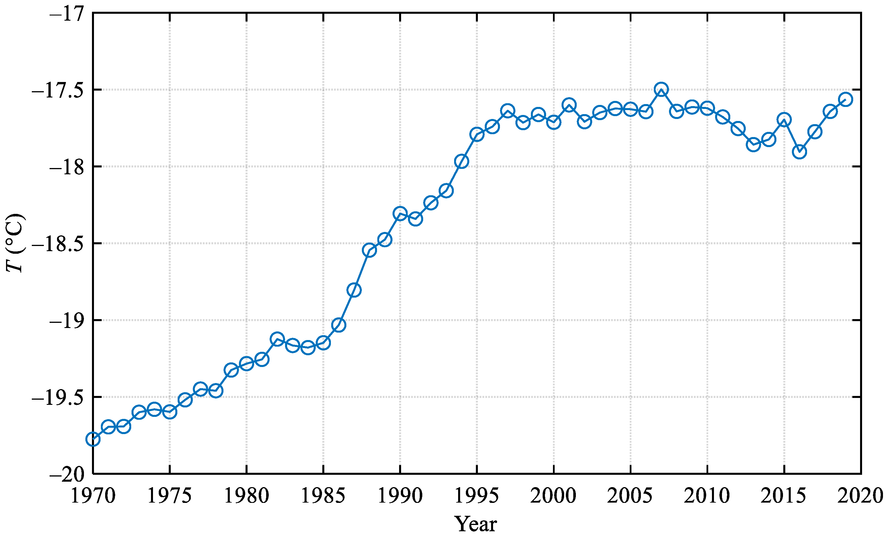
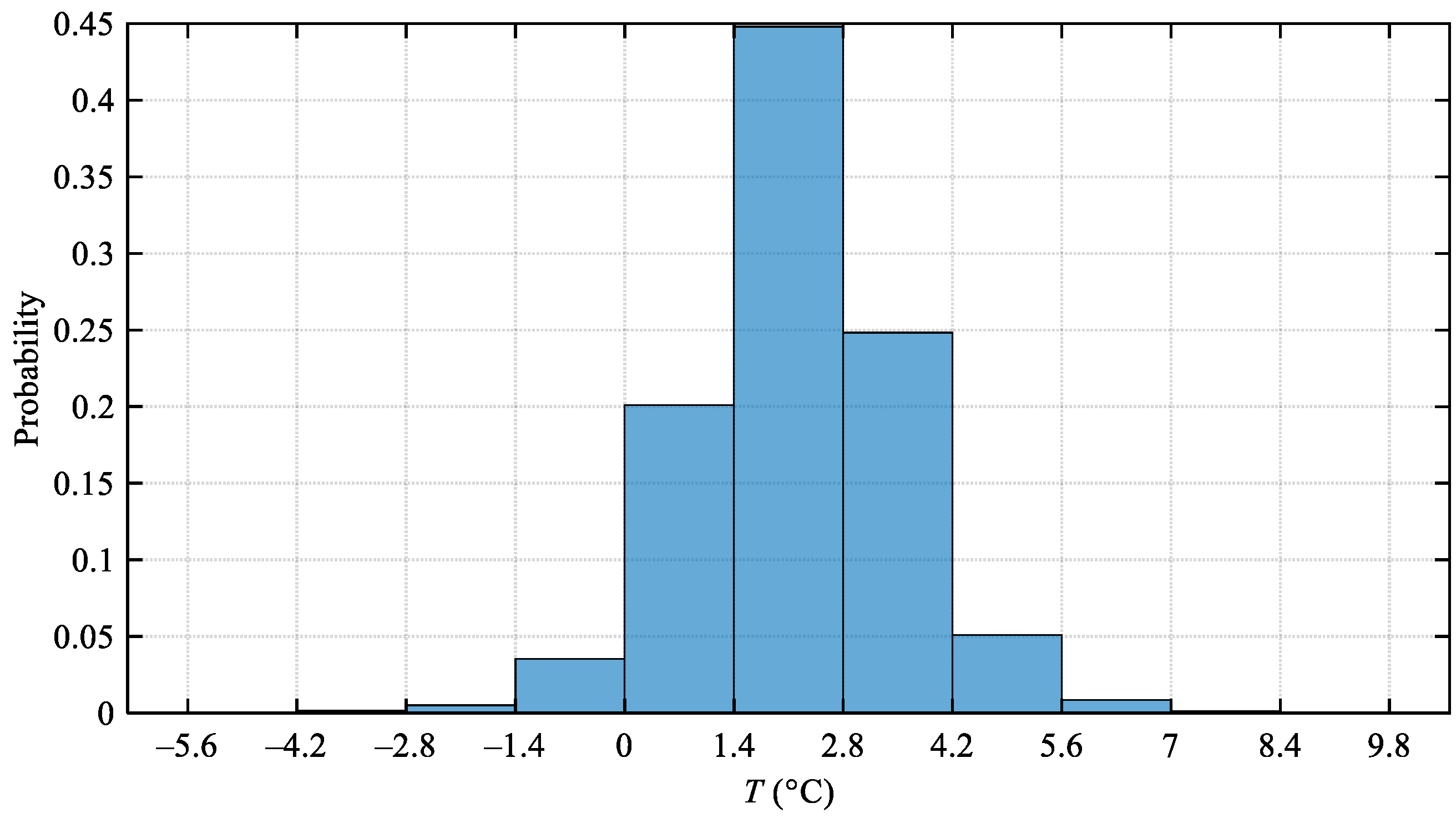
3. Impact of Temperature Rise on Asphalt Pavement in China from 1970 to 2019

3.1. Data Basis

The meteorological data used in this paper were provided by the China Meteorological Data Service Centre, which include data collected from 699 meteorological stations around China from 1961 to 2019. Firstly, the five temperature-related parameters, k_T1, k_T2, k_T3, T_pef, and T, were calculated according to the data of each 10 consecutive years for each station. Then, the spatial interpolation method of CoKriging was employed with consideration of the station elevation to interpolate the parameters year-by-year. Finally, the 5 km × 5 km grid data covering China corresponding to each parameter and each year were obtained, which are the data basis of this study.

It should be noted that the number of meteorological stations with complete data is not entirely consistent across years. The difference in the number of included meteorological stations will affect the local spatial interpolation results, thereby compromise the reliability of change analysis to a certain extent. For example, a station has the observations of relevant indicators in a certain year. It will dominate the interpolations of that year in nearby areas. If in the following year, the observations of this station are missing. The interpolations in the areas around the station will be dominated by the other nearby stations. In this case, the changes of the indicators between the two years can’t be fully attributed to climate change because the data process is also a source of the changes. Therefore, only the stations with complete observations from 1961 through 2019 were retained in the analysis. Finally, 600 stations were included in the analysis of k_T1, k_T2, k_T3, and T_pef, and 597 stations were included in the analysis of T.

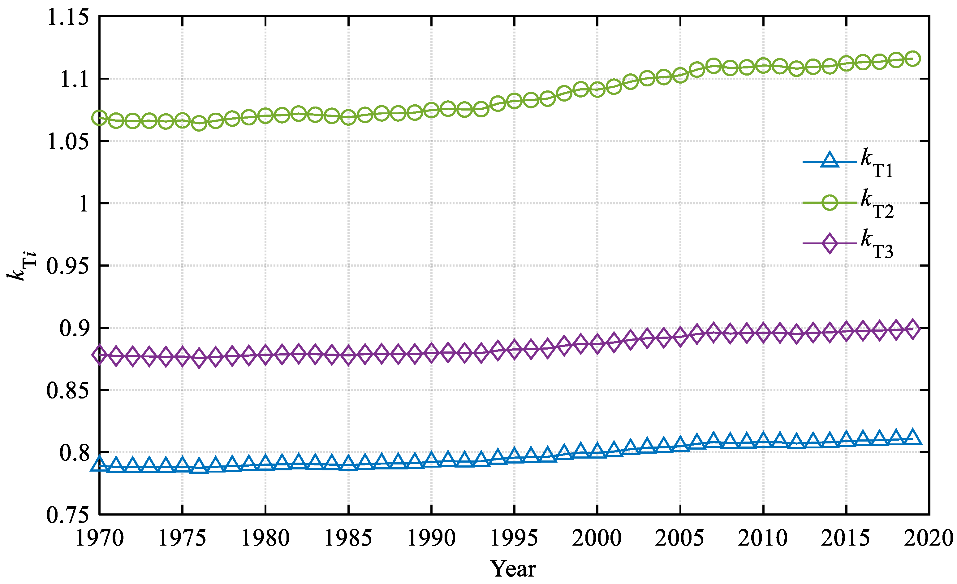
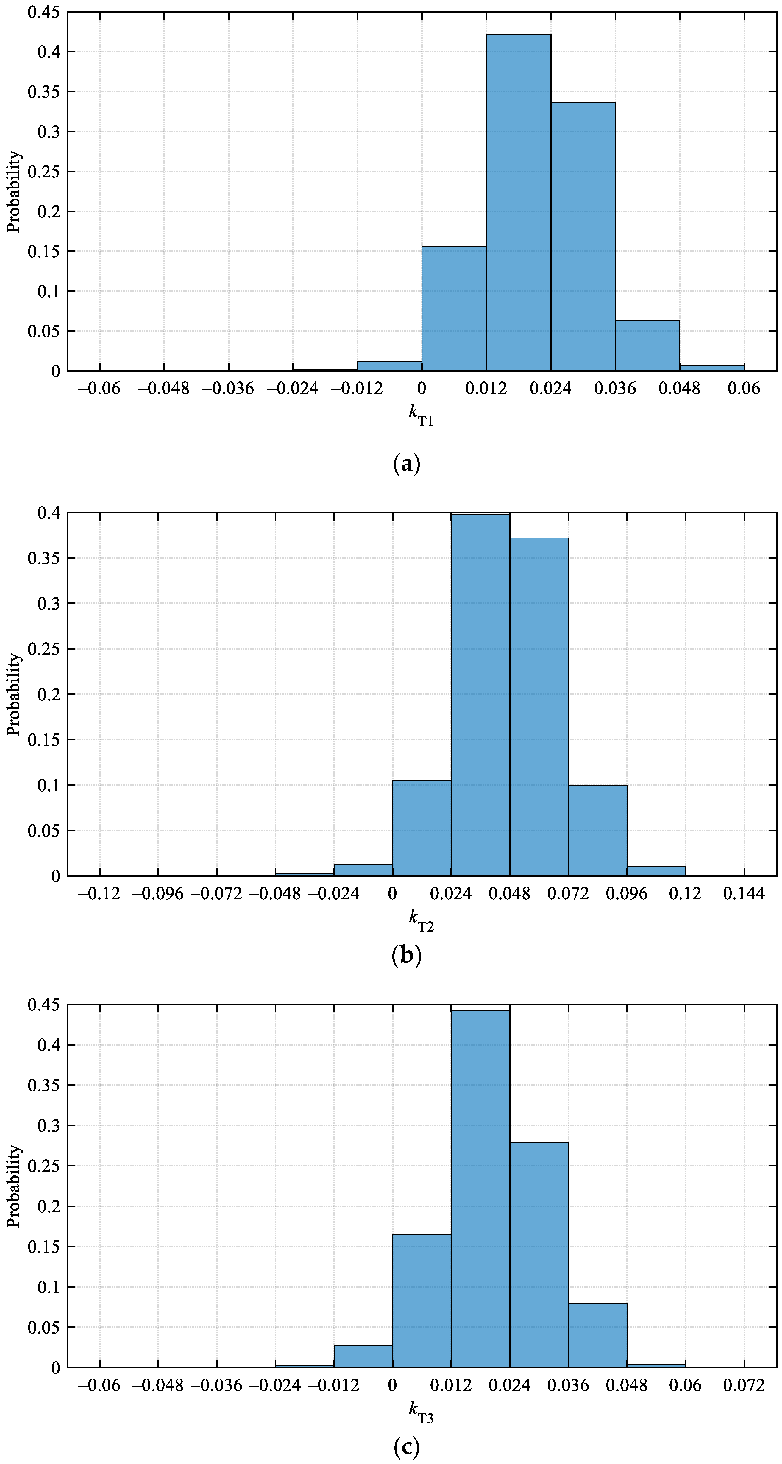
3.2. Impact on the FLAL, FLIBSL, and AVCSSS

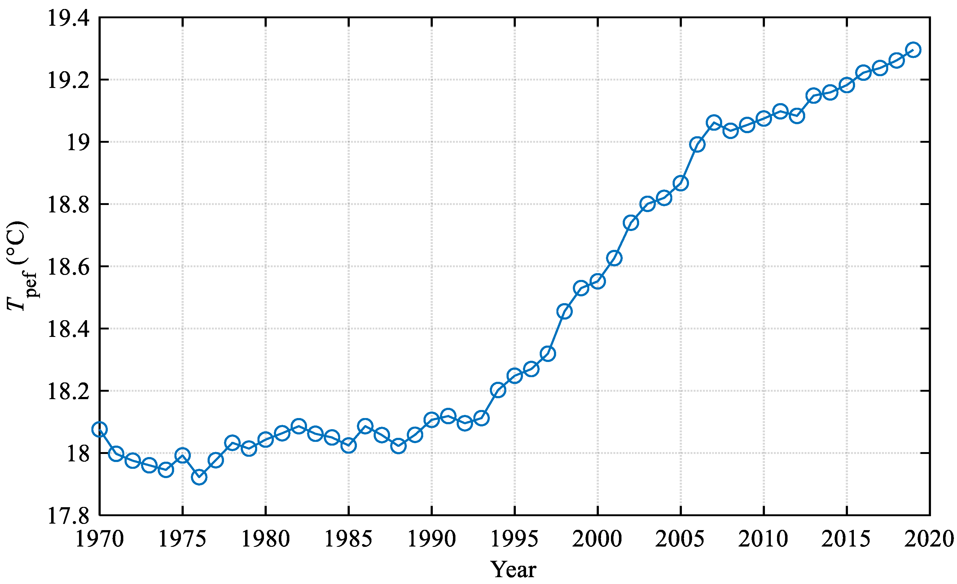
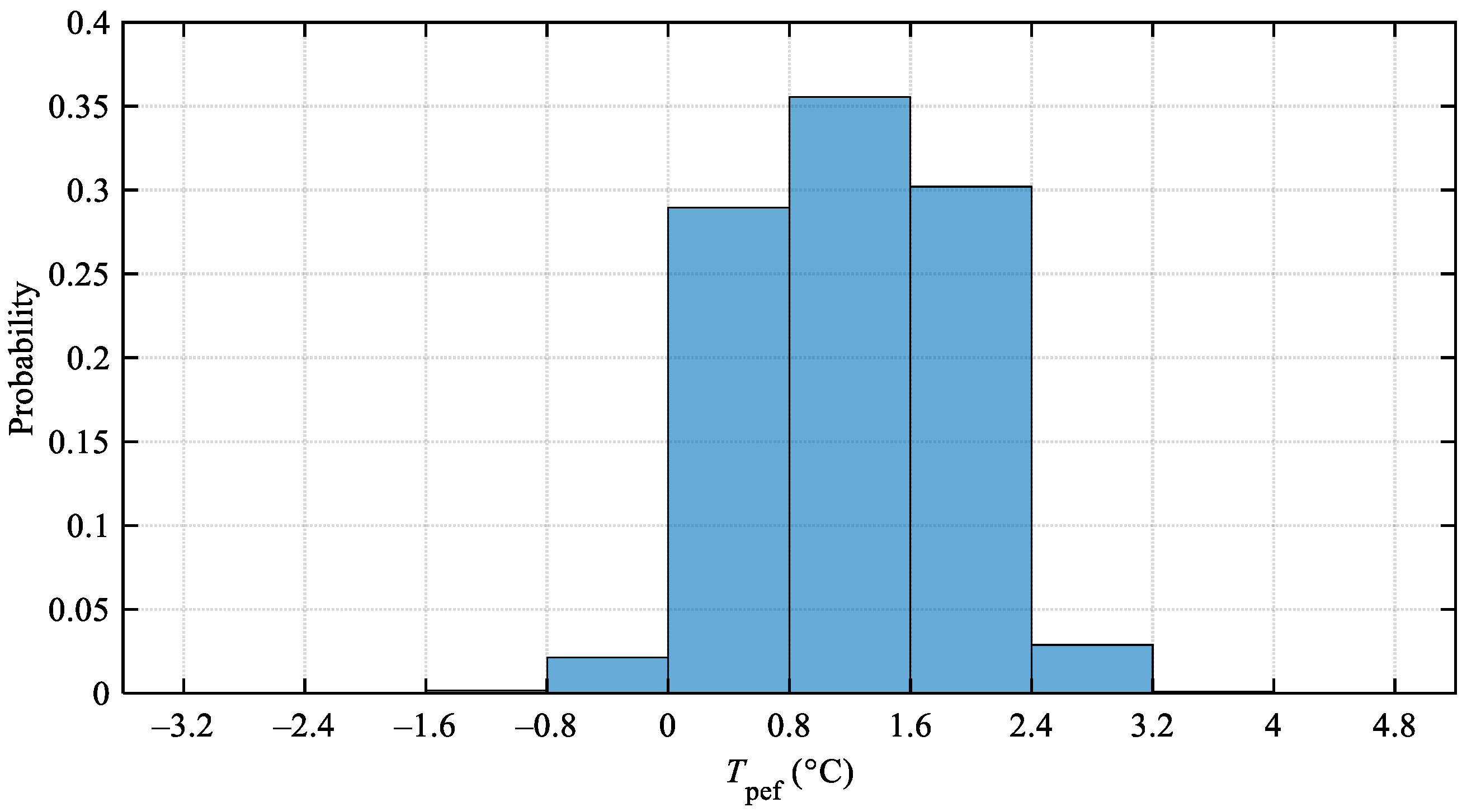
Figure 1 depicts the trend of China national means of k_T1, k_T2, and k_T3 from 1970 to 2019. As can be seen, all the three temperature calibration coefficients kept relatively stable before 1992, and increased year by year after that. From 1970 to 2019, the total increase in k_T1 is 0.0216. The increase by 1992 is only 0.003. The corresponding increase percentages in 1992 and 2019 are 0.43% and 2.74% respectively. The total increase in k_T2 is 0.0475 from 1970 to 2019. The increase from 1992 to 2019 is 0.0409. The k_T2 increased by 0.62% and 4.45% in 1992 and 2019, respectively, compared to 1970. The total increase in k_T3 was 0.0205 from 1970 to 2019, including 0.0014 from 1970 to 1992. In 1992 and 2019, it increased by 0.16% and 2.33%, respectively, compared to 1970.

The histograms of the differences in k_T1, k_T2, and k_T3 between 1970 and 2019 for China are depicted in Figure 2, which helps understand the change distribution of the three coefficients around China. As can be seen from Figure 2a, in 2019, only 1.41% of regions of China had a decrease or no change in k_T1 compared to 1970, and the decreases were mainly between 0 and 0.012. A total of 98.59% of the regions of China experienced an increase to various degrees. The increases of most regions were between 0.012 and 0.036. The regions with increases between 0.012 and 0.024 and between 0.024 and 0.036 accounted for 44.20% and 33.70% of China’s land, respectively. A total of 7.08% of regions of China even had a rise of more than 0.036.

It is shown in Figure 2b that only 1.38% of the regions of China experienced a decrease or no change in k_T2 from 1970 to 2019, of which the decreases were mainly between 0 and 0.024. A total of 98.62% of the regions of China showed different degrees of increase, of which the regions with increases between 0.024 and 0.048 and between 0.048 and 0.072 accounted for 39.75% and 37.25% of China’s land, respectively. There was also 11.07% of China’s land with an increase of more than 0.072.

It can be seen from Figure 2c that k_T3 decreased or remained unchanged in only 3.01% of the regions of China from 1970 to 2019. Most of the decreases were between 0 and 0.012. A total of 96.99% of the regions of China experienced an increase. The increases mainly ranged from 0 to 0.036. The regions with increases between 0 and 0.012, 0.012 and 0.024, and 0.024 and 0.036 accounted for 16.54%, 44.24%, and 27.84% of China’s total land, respectively. Some regions even saw an increase of more than 0.036, which accounted for 8.37% of the total land of China.

In the prediction models of the FLAL, FLIBSL, and AVCSSS, shown in Equations (1)–(3), the impact of temperature conditions is represented by a linear coefficient, which is a power function of the corresponding temperature calibration coefficient. Thus, by fixing the parameters except for the temperature calibration coefficients, the impact of the changes of temperature conditions on the FLAL, FLIBSL, and AVCSSS can be quantitatively evaluated by Equations (14)–(16), respectively.

$$\mathrm{The}\mathrm{impact}\mathrm{of}{k}_{T1}\mathrm{change}\mathrm{on}\mathrm{FLAL}=\left(\frac{k_{T1\cdot Year2}^{-1}-k_{T1\cdot Year1}^{-1}}{k_{T1\cdot Year1}^{-1}}\right)\times 100\%$$

(14)

$$\mathrm{The}\mathrm{impact}\mathrm{of}{k}_{T2}\mathrm{change}\mathrm{on}\mathrm{FLIBSL}=\left(\frac{k_{T2\cdot Year2}^{-1}-k_{T2\cdot Year1}^{-1}}{k_{T2\cdot Year1}^{-1}}\right)\times 100\%$$

(15)

$$\mathrm{The}\mathrm{impact}\mathrm{of}{k}_{T3}\mathrm{change}\mathrm{on}\mathrm{AVCSSS}=\left(\frac{k_{T3\cdot Year2}^{-0.21}-k_{T3\cdot Year1}^{-0.21}}{k_{T3\cdot Year1}^{-0.21}}\right)\times 100\%$$

(16)

The FLAL decreased on average by 0.43% from 1970 to 1992 and by 2.66% from 1970 to 2019 due to the increase in national mean k_T1. With the increase in national mean k_T2, the FLIBSL decreased on average by 0.62% from 1970 to 1992 and by 4.26% from 1970 to 2019. Due to the increase in k_T3, the AVCSSS decreased by 0.03% on average from 1970 to 1992, and by 0.48% from 1970 to 2019. The above data show that the change in temperature conditions since 1961 in China has had a slight influence on the fatigue life of asphalt pavement. The influence degrees are within 5%. The AVCSSS decreased by less than 0.5%, which means the change in temperature conditions has had no obvious effect on it.

3.3. Impact on PDAL

Figure 3 shows the variation in China’s national mean T_pef from 1970 to 2019. As shown, the increasing trend was very obvious. From 1970 to 1992, the T_pef was relatively stable. After 1992, the T_pef showed rapid growth. The growth rate slowed down after 2007. From 1970 to 2019, the total increase in T_pef was 1.22 °C. The increases before and after 1992 were 0.02 °C and 1.2 °C, respectively. The T_pef increased by 6.63% in 2019 compared to 1992.

Figure 4 is the histogram of the difference in T_pef between 1970 and 2019 for China. As can be seen, the T_pef showed a decrease or no change in 2019 compared to 1970 in only 2.26% of the regions of China. The decreases were mainly between 0 °C and 0.8 °C. A total of 97.74% of the regions of China experienced various degrees of increase. The increases in most regions were between 0 °C and 2.4 °C. The regions with increases between 0.8 °C and 1.6 °C and between 1.6 °C and 2.4 °C accounted for 35.52% and 30.22% of China’s land, respectively. The regions with an increase of more than 2.4 °C accounted for 2.98%.

As shown in Equations (9) and (10), a power function of T_pef is included as a linear coefficient in the PDAL prediction model to reflect the impact of temperature conditions. Then the impact of the change of temperature conditions on the PDAL can be qualified according to Equation (17).

$$\mathrm{The}\mathrm{impact}\mathrm{of}{T}_{pef}\mathrm{change}\mathrm{on}\mathrm{PDAL}=\left(\frac{T_{pef\cdot Year2}^{2.93}-T_{pef\cdot Year1}^{2.93}}{T_{pef\cdot Year1}^{2.93}}\right)\times 100\%$$

(17)

It was calculated that the PDAL increased on average by 20.70% from 1992 to 2019 due to the increase in national mean T_pef. It is shown that the change in temperature conditions from 1983 to 2019 resulted in a very significant impact on the PDAL, which should attract more attention.

3.4. Impact on LTCIASL

Figure 5 depicts the variation of T from 1970 to 2019. Although the T showed slight fluctuations with year, its general increasing trend was very obvious. The T increased rapidly from 1970 to 1997, but remained stable after 1997. From 1970 to 2019, the total increase in T was 2.21 °C. The increase before 1997 was 2.14 °C. The T increased by 10.81% in 1997 compared to 1970. After 1997, the T kept relatively stable. It seems that the trend of T is not consistent with that of the national average winter temperature, which has been increasing since 1961 [41]. However, it should be noted that the increase in extreme weather events is a typical feature of climate change [2]. The pavement design low-temperature, T, is defined based on the annual extreme low temperature. Although the average winter temperature has been increasing since 1997, the extreme low temperature has not increased obviously. As a result, the pavement design low-temperature has remained relatively stable since 1997.

Figure 6 is the histogram of the difference in T between 1970 and 2019 for China. As can be seen, only 4.03% of the regions of China had a decrease or no change in T from 1970 to 2019. The decreases were between 0 °C and 1.4 °C. A total of 98.59% of the regions of China showed an increase in T to various extents. The regions with increases between 1.4 °C and 2.8 °C and between 2.8 °C and 4.2 °C accounted for 44.86% and 24.86% of China’s land, respectively. The regions with an increase of more than 4.2 °C accounted for 6.09%.

There is not a simple linear relationship between T and CI, in accordance with Equation (13). The impact of the change of climatic conditions on LTCIASL depends on some parameters of pavement structure, asphalt binder, and subgrade type. Take the benchmark asphalt pavement structure with an inorganic binder stabilized material base and sandy soil subgrade into consideration, where h_a is 180 mm, and b is 5. Take S_t as 300 MPa, and according to Equation (13), the value of CI is 1.89 with the national mean T of −19.8 °C in 1970, which meets the requirement of no larger than 3 for expressways and first-grade highways in JTG D50-2017 [40]. Based on this, when the national mean T reached −17.6 °C in 1997, the CI decreased to 1.49, by 20.99% compared to 1970. Although this result will change with different parameters, it can be concluded that the change in temperature conditions from 1970 to 1997 significantly alleviated the low-temperature cracking of asphalt pavement. However, there was almost no impact on the LTCIASL after 1997 since the national mean T remained stable.

4. Potential Impact of Global Warming on Asphalt Pavement in China in the Future

Although it is a widespread concern, climate change is still difficult to control. According to the sixth assessment report of the IPCC [2], the GMST is very likely to reach 1.5 °C above pre-industrial levels before 2040 even under the very low emission scenarios (the Shared Socio-economic Pathway 1–1.9 (SSP1-1.9)). The GMST anomaly is very likely to reach 2.0 °C before 2060 under the intermediate scenario (SSP2-4.5) [2]. Therefore, it is necessary to evaluate the potential impact of global warming of 1.5 °C and 2.0 °C on asphalt pavement.

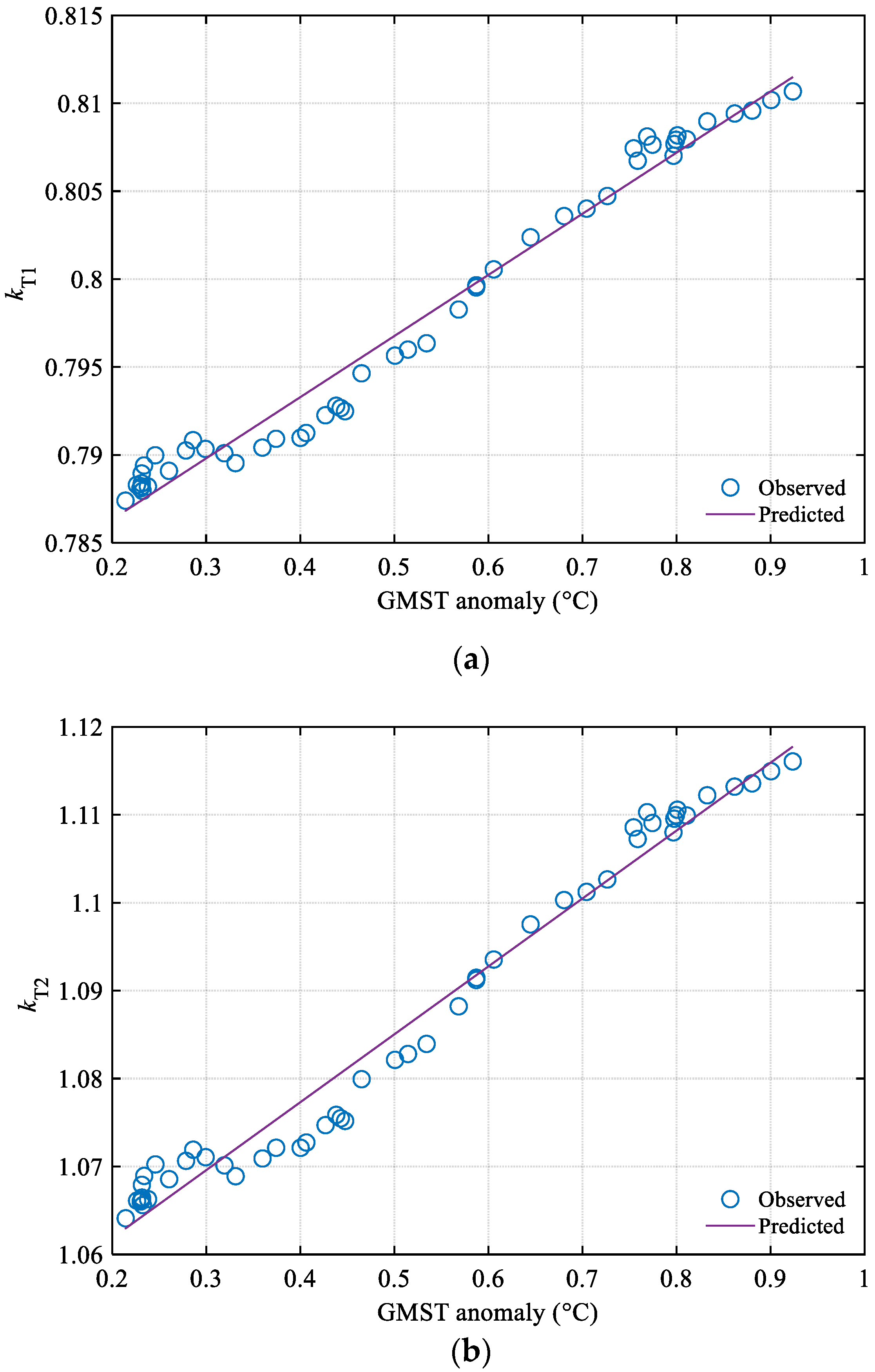
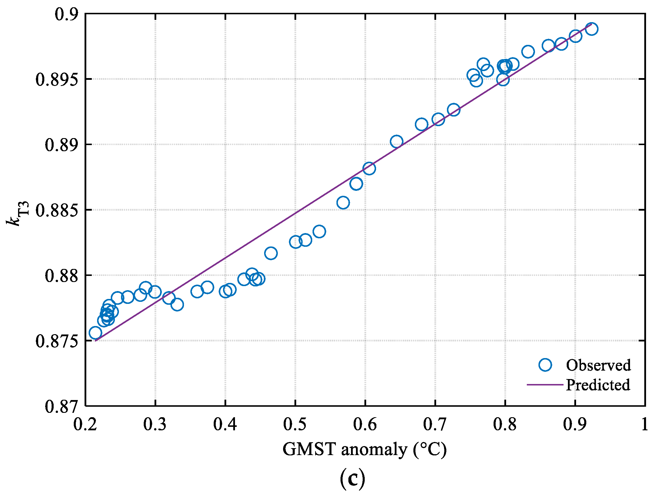
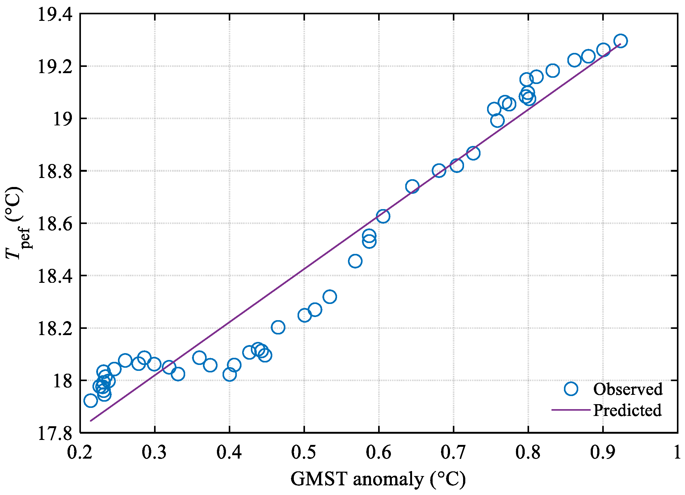
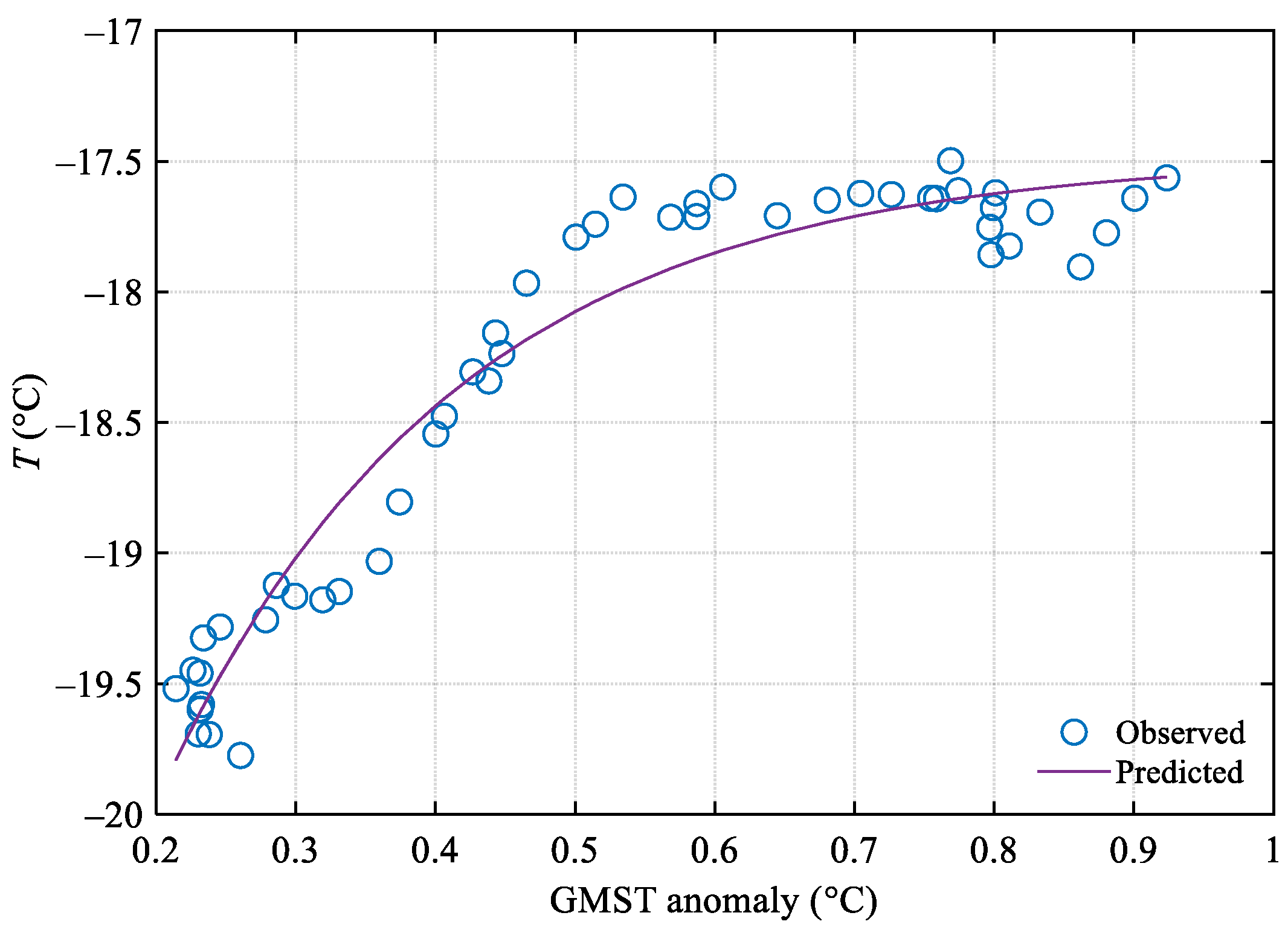
4.1. Relationship between GMST Anomaly and Temperature-Related Parameters for Asphalt Pavement Performance Prediction in China

The GMST anomaly is a commonly used parameter representing the level of global warming. Many agencies have constructed GMST models and release relevant data regularly, which include the Met Office Hadley Centre and the Climatic Research Unit of the University of East Anglia (UK), the National Oceanic and Atmospheric Administration (USA), the Goddard Institute for Space Studies of the National Aeronautics and Space Administration (USA), the European Centre for Medium-Range Weather Forecasts, and the Japan Meteorological Agency [42]. The data released by the Met Office Hadley Centre and the Climatic Research Unit of the University of East Anglia, HadCRUT4, have a relatively long time span, which include the GMST data since 1850. The HadCRUT4 was employed in this paper to calculate the GMST anomaly to pre-industrial (1850–1900) levels. Then, the relationships between GMST anomaly and temperature-related parameters for asphalt pavement performance prediction were investigated by using statistical regression analysis. It should be noted that the averages of 10 consecutive years of the GMST anomaly were used in the analysis to match the temperature-related parameters.

It was found that there are good linear relationships between GMST anomaly and China national means of k_T1, k_T2, k_T3, and T_pef. The relationship between GMST anomaly and China national mean T can be presented well by an exponential model. Figure 7, Figure 8 and Figure 9 depict the relationships between GMST anomaly and China national means of k_T1, k_T2, k_T3, T_pef, and T, and

Table 1. Regression analysis results and models between temperature-related parameters and GMST anomaly.

Parameter	Regression Model	R Square	F Value	p <
kT1	$y=0.0348x+0.7794$	0.9770	2078.5	0.0001
kT2	$y=0.0772x+1.0464$	0.9747	1887.2	0.0001
kT3	$y=0.0341x+0.8677$	0.9603	1187.6	0.0001
Tpef	$y=2.0291x+17.4106$	0.9464	865.9	0.0001
T	$y=-6.3934e^{\frac{-x}{0.2105}}-17.4810$	0.9441	396.6	0.0001

lists the corresponding regression models and statistical analysis results. In the regression models, x and y represent the GMST anomaly (°C) and the corresponding temperature-related parameter, respectively. As shown in Table 1, the significant levels of all models are higher than 0.0001 and all the R-square values are above 0.94, which indicates that all the models have high reliability.

4.2. Potential Impact of 1.5 °C and 2 °C Global Warming on Asphalt Pavement in China in the Future

The changes to each temperature-related parameter for asphalt pavement performance prediction in China corresponding to the GMST anomaly of 1.5 °C or 2.0 °C can be estimated according to the models listed in Table 1. Then, the potential impact of the GMST anomaly of 1.5 °C or 2.0 °C on asphalt pavement in China can be assessed by using the methods presented in Section 3.

Table 2. Potential changes in asphalt pavement performance compared to 2019.

Design Indicator	1.5 °C GMST Anomaly	2 °C GMST Anomaly
Nf1	−2.52%	−4.51%
Nf2	−3.98%	−7.06%
[εz]	−0.46%	−0.85%
Ra	18.63%	36.71%
CI	−0.97%	−1.03%

lists the potential changes in asphalt pavement performance compared to 2019 when the GMST anomaly reaches 1.5 °C or 2.0 °C. It is shown that the most significant impact is on the PDAL. The 1.5 °C GMST anomaly means a PDAL increase of 18.63% compared to 2019, whereas 2.0 °C means 36.71%. When the GMST anomaly reaches 2.0 °C, the FLIBSL will be reduced by 7.06% compared to 2019, and the FLAL will decrease by 4.51%. The potential impacts of the GMST anomaly of 2.0 °C on the AVCSSS and the LTCIASL are about 1%, which are negligible.

It should be noted that the estimates here are based on China’s national means of k_T1, k_T2, k_T3, T_pef, and T. As shown in Figure 2, Figure 4 and Figure 6, these parameters have significant spatial variability. Therefore, some regions will experience more serious impacts.

In addition, according to the results listed in Table 2, the PDAL becomes more severe with the rise of GMST, but the LTCIASL remains almost unchanged. This means that the service temperature range of asphalt pavement will become wider in the future, which will bring severe challenges to the structure and material design of asphalt pavement.

5. Discussion

According to Equations (4)–(6) and Equation (11), k_T1, k_T2, k_T3, and T_pef are related not only to climatic conditions, but also to pavement structure. Though T is just a climatic indicator, the change in CI caused by the change in T also depends on pavement structure and material, in accordance with Equation (13). It should be noted that the preceding analysis is based on the benchmark asphalt pavement structure with an inorganic binder stabilized material base proposed in JTG D50-2017 [40]. The impact of the GMST anomaly may be different for various pavement structures. It is necessary to discuss it further.

The assessment presented in Section 4 was expanded through a series of trial calculations according to various reasonable pavement structures so that the influence of pavement structure on the assessment results can be understood. As shown in Equations (4)–(6), the temperature calibration coefficients of k_T1, k_T2, and k_T3 depend on the pavement structure parameters of $h_a^{\ast }/h_b^{\ast }$ and $E_a^{\ast }/E_b^{\ast }$. The trial calculations show that compared with 2019, the variation range of FLAL due to 1.5 °C and 2.0 °C GMST anomalies is about −1% to −3% and −3% to −5%, respectively. For the FLIBSL, the variation range is about 3% to 5.5% and 6% to 9%, respectively. For the AVCSSS, the variation ranges corresponding to 1.5 °C and 2.0 °C GMST anomalies are all below 1%. According to Equation (11), the T_pef shows a positive linear relationship with the total depth of asphalt layers, h_a. When h_a decreases from 400 mm to 40 mm, compared with 2019, the increase rate of PDAL corresponding to 1.5 °C GMST anomaly will increase from 15.62% to 21.24%. That corresponding to a 2.0 ˚C GMST anomaly will increase from 30.55% to 42.10%. Though the LTCIASL is related to S_t, b, and h_a besides T, the changes in S_t, b, and h_a have little impact on the preceding analysis result.

6. Conclusions

The impact of temperature rise on asphalt pavement in China in past decades was assessed by the performance prediction models for asphalt pavement based on the historical climate data. Furthermore, the relationships between temperature-related parameters and the GMST anomaly were established. The potential impact of 1.5 °C and 2.0 °C global warming on asphalt pavement in China was assessed accordingly. Some findings can be concluded as follows.

(1) The various aspects of asphalt pavement performance are significantly different in sensitivity to global warming. The PDAL increased on average by 20.70% from 1992 to 2019. The LTCIASL decreased on average by 20.99% in 1997 compared to 1970, but has remained almost unchanged since 1997. The FLAL and FLIBSL decreased by 0.43% and 0.62% from 1970 to 1992 and by 2.66% and 4.26% from 1970 to 2019, respectively. The AVCSSS decreased by less than 0.5% from 1970 to 2019.

(2) All the temperature-related parameters for asphalt pavement performance prediction in China have a good correlation with the GMST anomaly. The regression models between those parameters and GMST anomaly can be employed to estimate the potential impact of global warming on asphalt pavement in the future.

(3) When the GMST anomaly reaches 1.5 °C, the FLIBSL will be reduced by 3.98% compared to 2019, and the FLAL will decrease by 2.52%. The GMST anomaly of 2.0 °C will bring a decrease of 7.06% to the FLIBSL and a decrease of 4.51% to the FLAL. The GMST anomaly of 2.0 °C will bring only about 1% variations to the AVCSSS and LTCIASL, which are negligible.

(4) The PDAL will increase on average by 18.63% compared to 2019 when the GMST anomaly reaches 1.5 °C in the future. The GMST anomaly of 2.0 °C will bring the PDAL an increase of 36.71%. However, the increase in GMST in the future will not further alleviate the LTCIASL, which indicates a wider service temperature range of asphalt pavement and brings severe challenges to the structure and material design of asphalt pavement.

References

1. The National Academy of Sciences; The Royal Society. Climate Change: Evidence and Causes, Update 2020; The National Academy of Sciences: Washington, DC, USA; The Royal Society: London, UK, 2020. [Google Scholar]
2. IPCC. Climate Change 2021: The Physical Science Basis; Intergovernmental Panel on Climate Change: Geneva, Switzerland, 2021. [Google Scholar]
3. Taylor, K.E.; Stouffer, R.J.; Meehl, G.A. An Overview of CMIP5 and the Experiment Design. Bull. Am. Meteorol. Soc. 2012, 93, 485–498. [Google Scholar] [CrossRef] [Green Version]
4. Giorgi, F.; Coppola, E.; Solmon, F.; Mariotti, L.; Sylla, M.B.; Bi, X.; Elguindi, N.; Diro, G.T.; Nair, V.; Giuliani, G.; et al. RegCM4: Model description and preliminary tests over multiple CORDEX domains. Clim. Res. 2012, 52, 7–29. [Google Scholar] [CrossRef] [Green Version]
5. Mearns, L.O.; Sain, S.; Leung, L.R.; Bukovsky, M.S.; McGinnis, S.; Biner, S.; Caya, D.; Arritt, R.W.; Gutowski, W.; Takle, E.; et al. Climate change projections of the North American Regional Climate Change Assessment Program (NARCCAP). Clim. Chang. 2013, 120, 965–975. [Google Scholar] [CrossRef] [Green Version]
6. Scinocca, J.F.; Kharin, V.V.; Jiao, Y.; Qian, M.W.; Lazare, M.; Solheim, L.; Flato, G.M.; Biner, S.; Desgagne, M.; Dugas, B. Coordinated global and regional climate modeling. J. Clim. 2016, 29, 17–35. [Google Scholar] [CrossRef]
7. Morice, C.P.; Kennedy, J.J.; Rayner, N.A.; Jones, P.D. Quantifying uncertainties in global and regional temperature change using an ensemble of observational estimates: The HadCRUT4 data set. J. Geophys. Res. Atmos. 2012, 117, D08101. [Google Scholar] [CrossRef]
8. Daniel, J.S.; Jacobs, J.M.; Douglas, E.; Mallick, R.B.; Hayhoe, K. Impact of climate change on pavement performance: Preliminary lessons learned through the infrastructure and climate network (ICNet). In Climatic Effects on Pavement and Geotechnical Infrastructure; Liu, J., Li, P., Zhang, X., Huang, B., Eds.; American Society of Civil Engineers (ASCE): Reston, VA, USA, 2014; pp. 1–9. [Google Scholar]
9. Austroads. Impact of Climate Change on Road Infrastructure; Austroads Incorporated: Sydney, Australia, 2004. [Google Scholar]
10. Austroads. Impact of Climate Change on Road Performance: Updating Climate Information for Australia; Austroads Incorporated: Sydney, Australia, 2010. [Google Scholar]
11. Valle, O.; Qiao, Y.; Dave, E.; Mo, W. Life cycle assessment of pavements under a changing climate. In Pavement Life-Cycle Assessment; Al-Qadi, I.L., Ozer, H., Harvey, J., Eds.; CRC Press: London, UK, 2017; pp. 241–250. [Google Scholar]
12. Knott, J.F.; Sias, J.E.; Dave, E.V.; Jacobs, J.M. Seasonal and Long-Term Changes to Pavement Life Caused by Rising Temperatures from Climate Change. Transp. Res. Rec. 2019, 2673, 267–278. [Google Scholar] [CrossRef]
13. Stoner, A.M.K.; Daniel, J.S.; Jacobs, J.M.; Hayhoe, K.; Scott-Fleming, I. Quantifying the Impact of Climate Change on Flexible Pavement Performance and Lifetime in the United States. Transp. Res. Rec. 2019, 2673, 110–122. [Google Scholar] [CrossRef]
14. Zareie, A.; Amin, M.S.R.; Amador-Jimenez, L.E. Thornthwaite Moisture Index Modeling to Estimate the Implication of Climate Change on Pavement Deterioration. J. Transp. Eng. 2016, 142, 04016007. [Google Scholar] [CrossRef]
15. Tighe, S.L.; Smith, J.; Mills, B.; Andrey, J. Evaluating Climate Change Impact an Low-Volume Roads in Southern Canada. Transp. Res. Rec. 2008, 2053, 9–16. [Google Scholar] [CrossRef]
16. Chen, X.; Wang, H.; Horton, R.; DeFlorio, J. Life-cycle assessment of climate change impact on time-dependent carbon-footprint of asphalt pavement. Transp. Res. Part D Transp. Environ. 2021, 91, 102697. [Google Scholar] [CrossRef]
17. Lu, D.; Tighe, S.L.; Xie, W. Pavement Risk Assessment for Future Extreme Precipitation Events under Climate Change. Transp. Res. Rec. 2018, 2672, 122–131. [Google Scholar] [CrossRef]
18. Mallick, R.B.; Jacobs, J.M.; Miller, B.J.; Daniel, J.S.; Kirshen, P. Understanding the impact of climate change on pavements with CMIP5, system dynamics and simulation. Int. J. Pavement Eng. 2018, 19, 697–705. [Google Scholar] [CrossRef]
19. Nakicenovic, N.; Alcamo, J.; Davis, G.; de Vries, B.; Fenhann, J.; Gaffin, S.; Gregory, K.; Griibler, A.; Jung, T.Y.; Kram, T.; et al. Special Report on Emissions Scenarios; Intergovernmental Panel on Climate Change: Geneva, Switzerland, 2000. [Google Scholar]
20. Moss, R.; Babiker, M.; Brinkman, S.; Calvo, E.; Carter, T.; Edmonds, J.; Elgizouli, I.; Emori, S.; Erda, L.; Hibbard, K.; et al. Towards New Scenarios for Analysis of Emissions, Climate Change, Impacts, and Response Strategies; Intergovernmental Panel on Climate Change: Geneva, Switzerland, 2008. [Google Scholar]
21. Wistuba, M.P.; Walther, A. Consideration of climate change in the mechanistic pavement design. Road Mater. Pavement 2013, 14, 227–241. [Google Scholar] [CrossRef]
22. Gudipudi, P.P.; Underwood, B.S.; Zalghout, A. Impact of climate change on pavement structural performance in the United States. Transp. Res. Part D Transp. Environ. 2017, 57, 172–184. [Google Scholar] [CrossRef]
23. Qiao, Y.; Santos, J.; Stoner, A.M.K.; Flinstch, G. Climate change impacts on asphalt road pavement construction and maintenance: An economic life cycle assessment of adaptation measures in the State of Virginia, United States. J. Ind. Ecol. 2020, 24, 342–355. [Google Scholar] [CrossRef]
24. Daniel, J.S.; Jacobs, J.M.; Miller, H.; Stoner, A.; Crowley, J.; Khalkhali, M.; Thomas, A. Climate change: Potential impacts on frost-thaw conditions and seasonal load restriction timing for low-volume roadways. Road Mater. Pavement 2018, 19, 1126–1146. [Google Scholar] [CrossRef]
25. Viola, F.; Celauro, C. Effect of climate change on asphalt binder selection for road construction in Italy. Transp. Res. Part D Transp. Environ. 2015, 37, 40–47. [Google Scholar] [CrossRef]
26. Li, Q.J.; Mills, L.; McNeil, S.; Attoh-Okine, N.O. Integrating potential climate change into the mechanistic-empirical based pavement design. Can. J. Civ. Eng. 2013, 40, 1173–1183. [Google Scholar] [CrossRef]
27. Mills, B.N.; Tighe, S.L.; Andrey, J.; Smith, J.T.; Huen, K. Climate change implications for flexible pavement design and performance in Southern Canada. J. Transp. Eng. 2009, 135, 773–782. [Google Scholar] [CrossRef]
28. Guest, G.; Zhang, J.; Maadani, O.; Shirkhani, H. Incorporating the impacts of climate change into infrastructure life cycle assessments: A case study of pavement service life performance. J. Ind. Ecol. 2020, 24, 356–368. [Google Scholar] [CrossRef]
29. Qiao, Y.; Dawson, A.R.; Parry, T.; Flintsch, G.W. Evaluating the effects of climate change on road maintenance intervention strategies and Life-Cycle Costs. Transp. Res. Part D Transp. Environ. 2015, 41, 492–503. [Google Scholar] [CrossRef]
30. Bilodeau, J.; Dore, G.; Drolet, F.P.; Chaumont, D. Correction of air freezing index for pavement frost protection design to consider future climate changes. Can. J. Civ. Eng. 2016, 43, 312–319. [Google Scholar] [CrossRef]
31. Steyn, W.J.M.; Pretorius, T. The potential effects of climate change on selected flexible South African pavements. In Sustainability, Eco-Efficiency, and Conservation in Transportation Infrastructure Asset Management; Losa, M., Papagiannakis, T., Eds.; CRC Press: London, UK, 2014; pp. 469–477. [Google Scholar]
32. Chai, G.; Van Staden, R.; Guan, H.; Kelly, G.; Chowdhury, S. The impacts of climate change on pavement maintenance in Queensland, Australia. In Materials and Infrastructures 2, 5B; Torrenti, J.M., La Torre, F., Eds.; ISTE Ltd.: London, UK, 2016; pp. 207–221. [Google Scholar]
33. Jiang, X.; Gabrielson, J.; Titi, H.; Huang, B.; Bai, Y.; Polaczyk, P.; Hu, W.; Zhang, M.; Xiao, R. Field investigation and numerical analysis of an inverted pavement system in Tennessee, USA. Transp. Geotech. 2022, 35, 100759. [Google Scholar] [CrossRef]
34. Qiao, Y.; Zhang, Y.; Zhu, Y.; Lemkus, T.; Stoner, A.M.K.; Zhang, J.; Cui, Y. Assessing impacts of climate change on flexible pavement service life based on Falling Weight Deflectometer measurements. Phys. Chem. Earth 2020, 120, 102908. [Google Scholar] [CrossRef]
35. Qiao, Y.; Zhang, Y.; Elshaer, M.; Daniel, J.S. A method to assess climate change induced damage on flexible pavements with machine learning. In Bearing Capacity of Roads, Railways and Airfields; Loizos, A., Al-Qadi, I.L., Scarpas, A.T., Eds.; CRC Press: London, UK, 2017; pp. 2103–2108. [Google Scholar]
36. Jeong, H.; Kim, H.; Kim, K.; Kim, H. Prediction of flexible pavement deterioration in relation to climate change using fuzzy logic. J. Infrastruct. Syst. 2017, 23, 04017008. [Google Scholar] [CrossRef]
37. Mallick, R.B.; Radzicki, M.J.; Daniel, J.S.; Jacobs, J.M. Use of system dynamics to understand long-term impact of climate change on pavement performance and maintenance cost. Transp. Res. Rec. 2014, 2455, 1–9. [Google Scholar] [CrossRef] [Green Version]
38. Chang, C.M.; Ortega, O. A methodology to quantify the impact of climate change on the state of good repair of pavements. In Bituminous Mixtures and Pavements VII; Nikolaides, A.F., Manthos, E., Eds.; CRC Press: London, UK, 2019; pp. 399–410. [Google Scholar]
39. Wang, Y.; Huang, Y.; Rattanachot, W.; Lau, K.K.; Suwansawas, S. Improvement of pavement design and management for more frequent flooding caused by climate change. Adv. Struct. Eng. 2015, 18, 487–496. [Google Scholar] [CrossRef]
40. Ministry of Transport, China. Specifications for Design of Highway Asphalt Pavement (JTG D50-2017); China Communications Press: Beijing, China, 2017. [Google Scholar]
41. Climate Change Center of China Meteorological Administration. The Blue Paper of Climate Change in China 2020; Science Press: Beijing, China, 2020. [Google Scholar]
42. World Meteorological Organization. WMO Statement on the State of the Global Climate in 2019; World Meteorological Organization: Geneva, Switzerland, 2020. [Google Scholar]
Figure 1. Trend of China’s national means of the 3 temperature calibration coefficients with year.
Sustainability 14 09044 g001
Figure 2. Histograms of the differences of the 3 temperature calibration coefficients between 1970 and 2019: (a) kT1; (b) kT2; (c) kT3.
Sustainability 14 09044 g002
Figure 3. Trend of China’s national mean of the equivalent temperature with year.
Sustainability 14 09044 g003
Figure 4. Histogram of the difference of the equivalent temperature between 1970 and 2019.
Sustainability 14 09044 g004
Figure 5. Trend of China’s national mean of the pavement design low-temperature with year.
Sustainability 14 09044 g005
Figure 6. Histogram of the difference in the pavement design low-temperature between 1970 and 2019.
Sustainability 14 09044 g006
Figure 7. Correlations between temperature calibration coefficients and GMST anomaly: (a) kT1; (b) kT2; (c) kT3.
Sustainability 14 09044 g007aSustainability 14 09044 g007b
Figure 8. Correlation between equivalent temperature and GMST anomaly.
Sustainability 14 09044 g008
Figure 9. Correlation between pavement design low-temperature and GMST anomaly.
Sustainability 14 09044 g009