
HLNet Model and Application in Crop Leaf Diseases Identification


Abstract
:1. Introduction
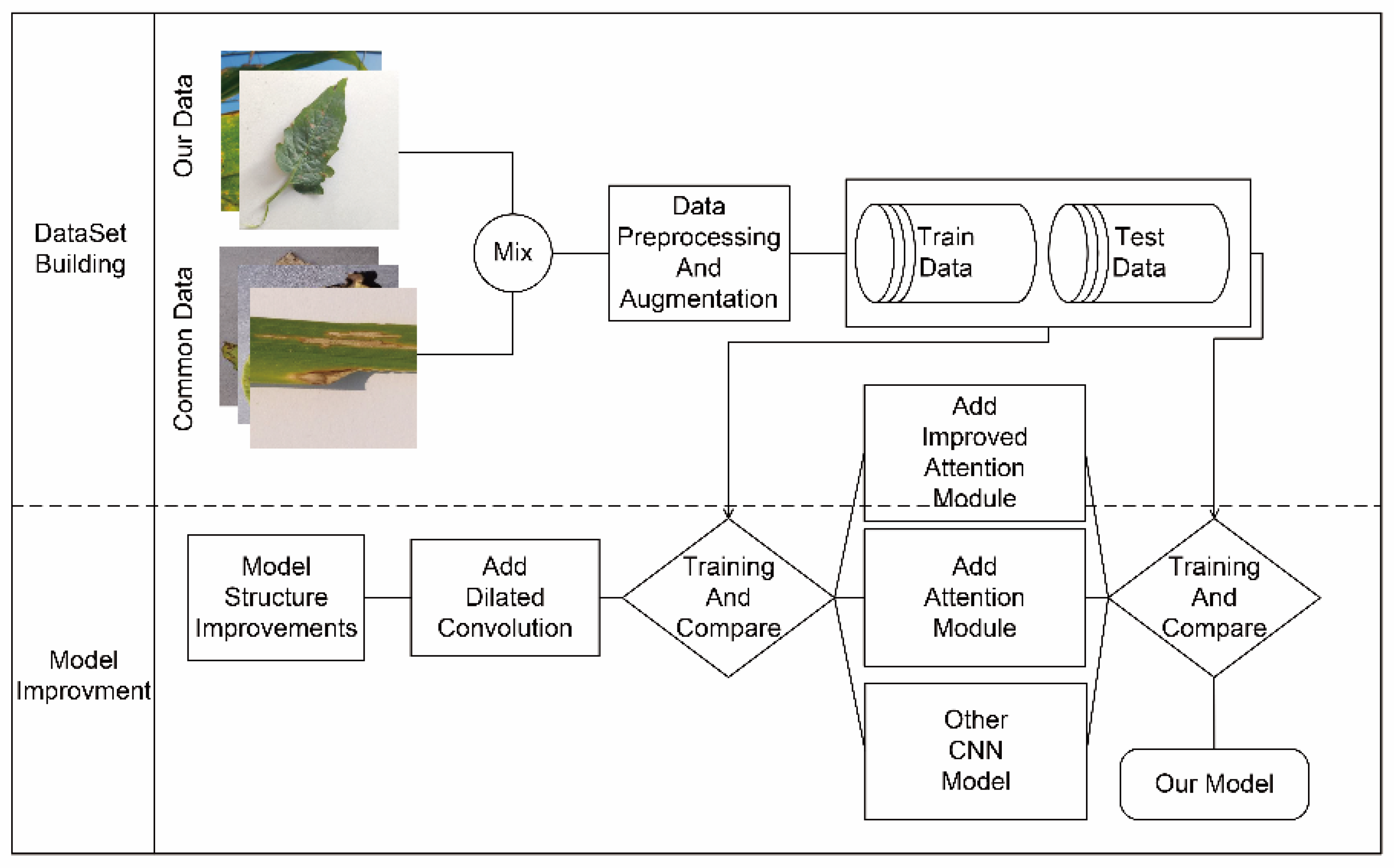
2. Materials and Methods
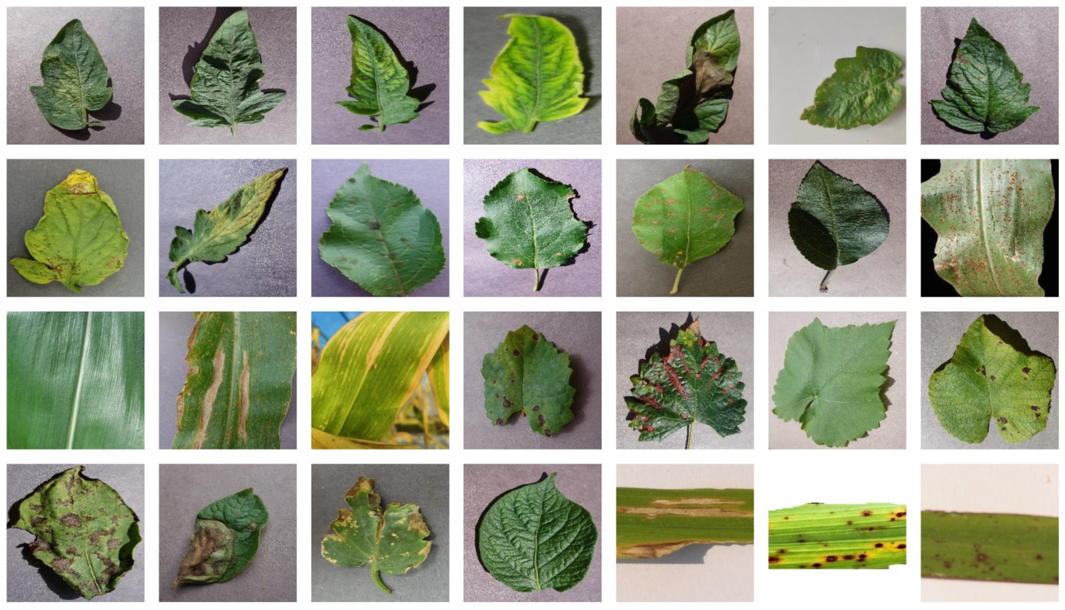
2.1. Dataset and Expansion
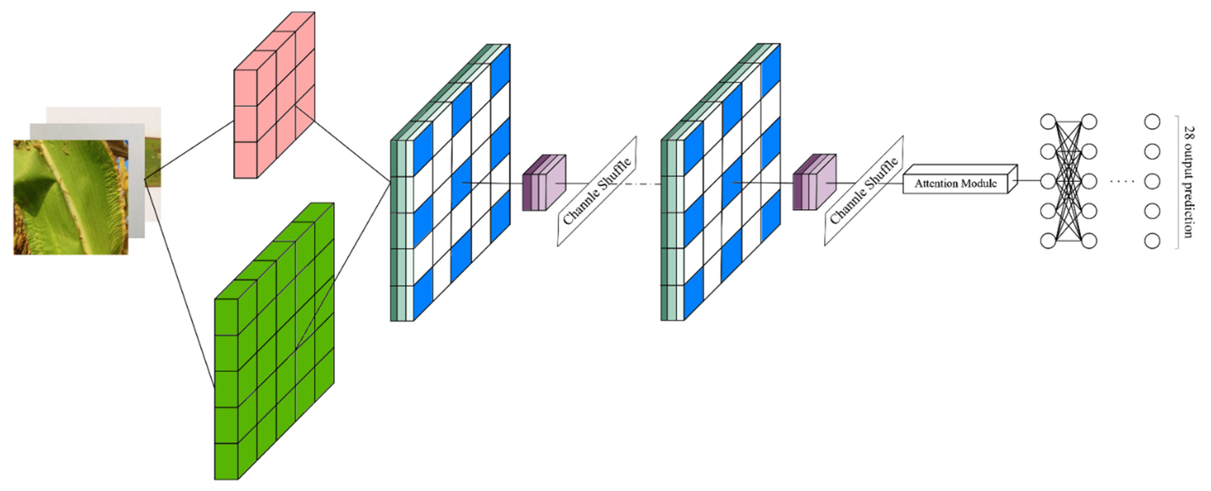
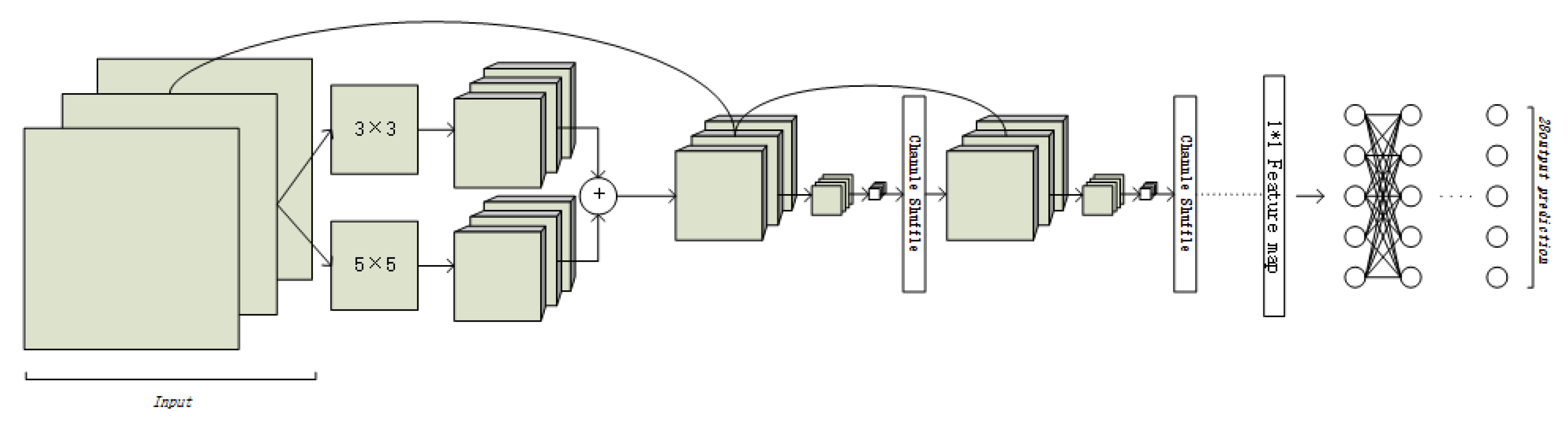
2.2. HLNet
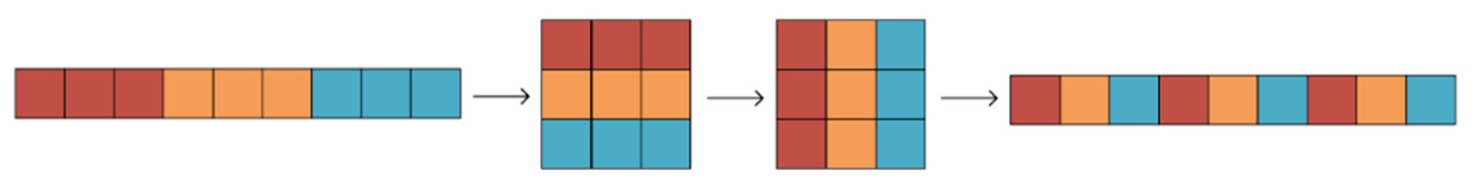
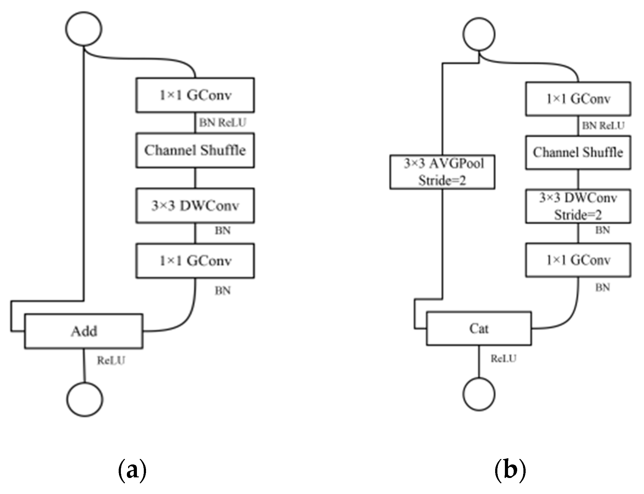
2.3. ShuffleNetV1
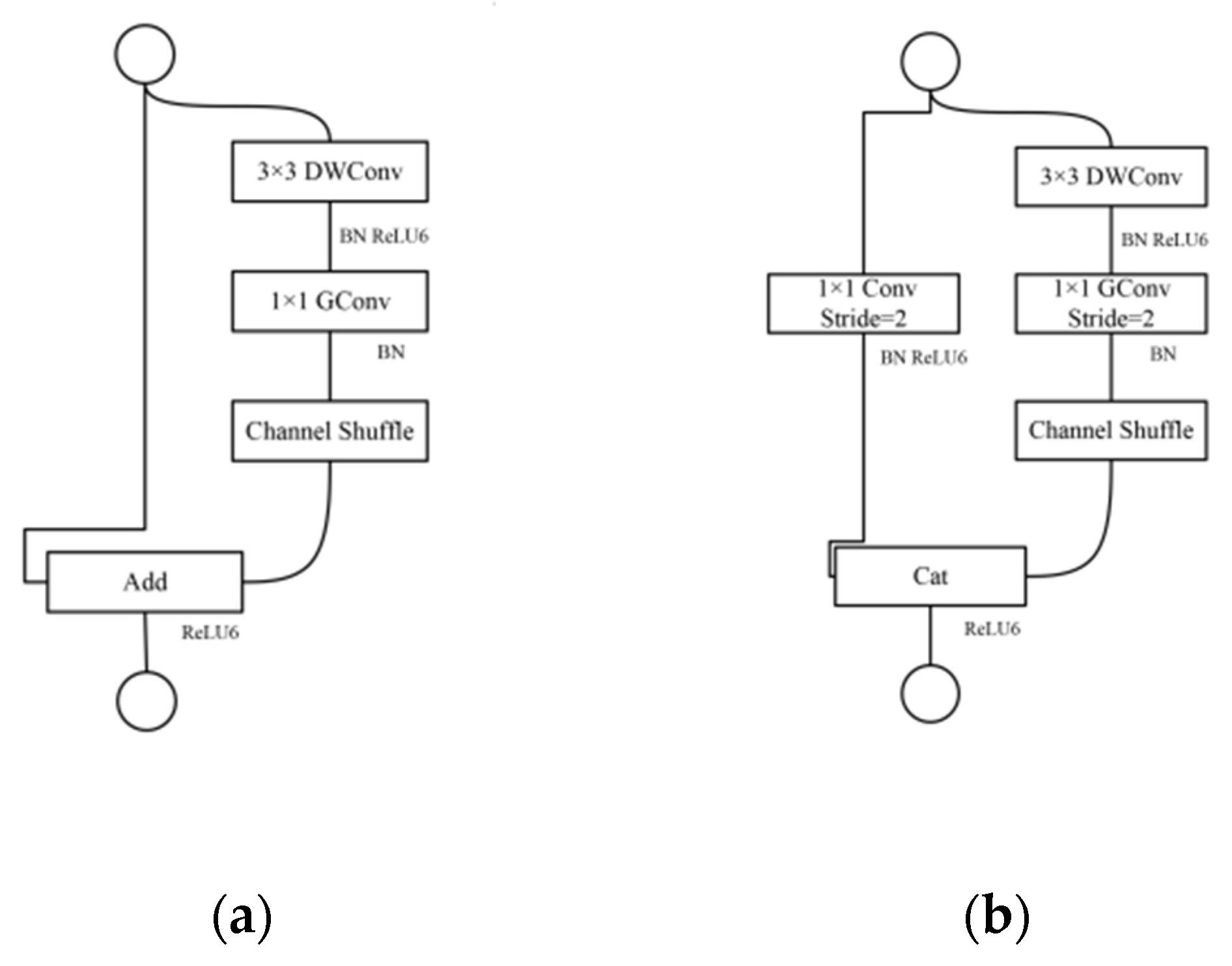
2.4. Improvements of ShuffleNetV1 Model
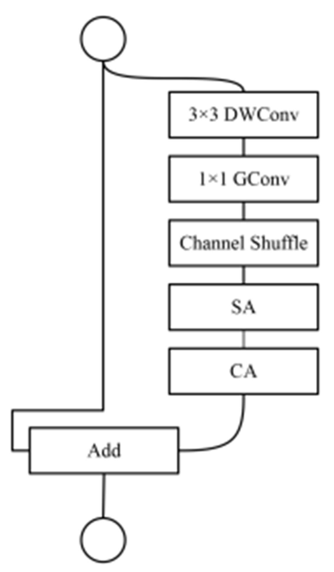
2.4.1. Block Improvement
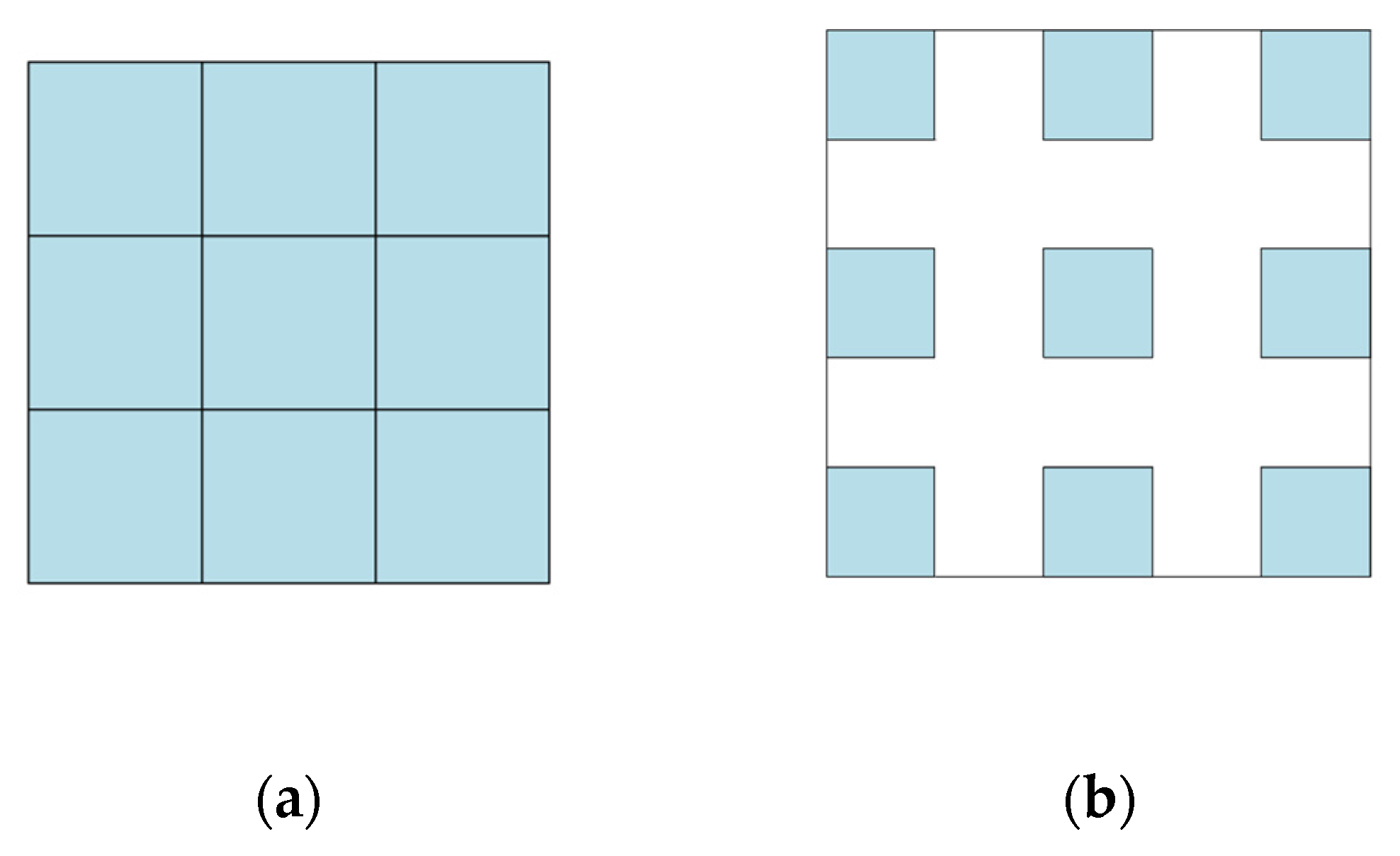
2.4.2. Dilated Convolution
2.5. Attention Module Improvements
2.5.1. Channel Attention and Spatial Attention
2.5.2. Model Based on Improved Attention
2.6. Experimental Environment Parameter Settings
3. Experimental Results and Analysis
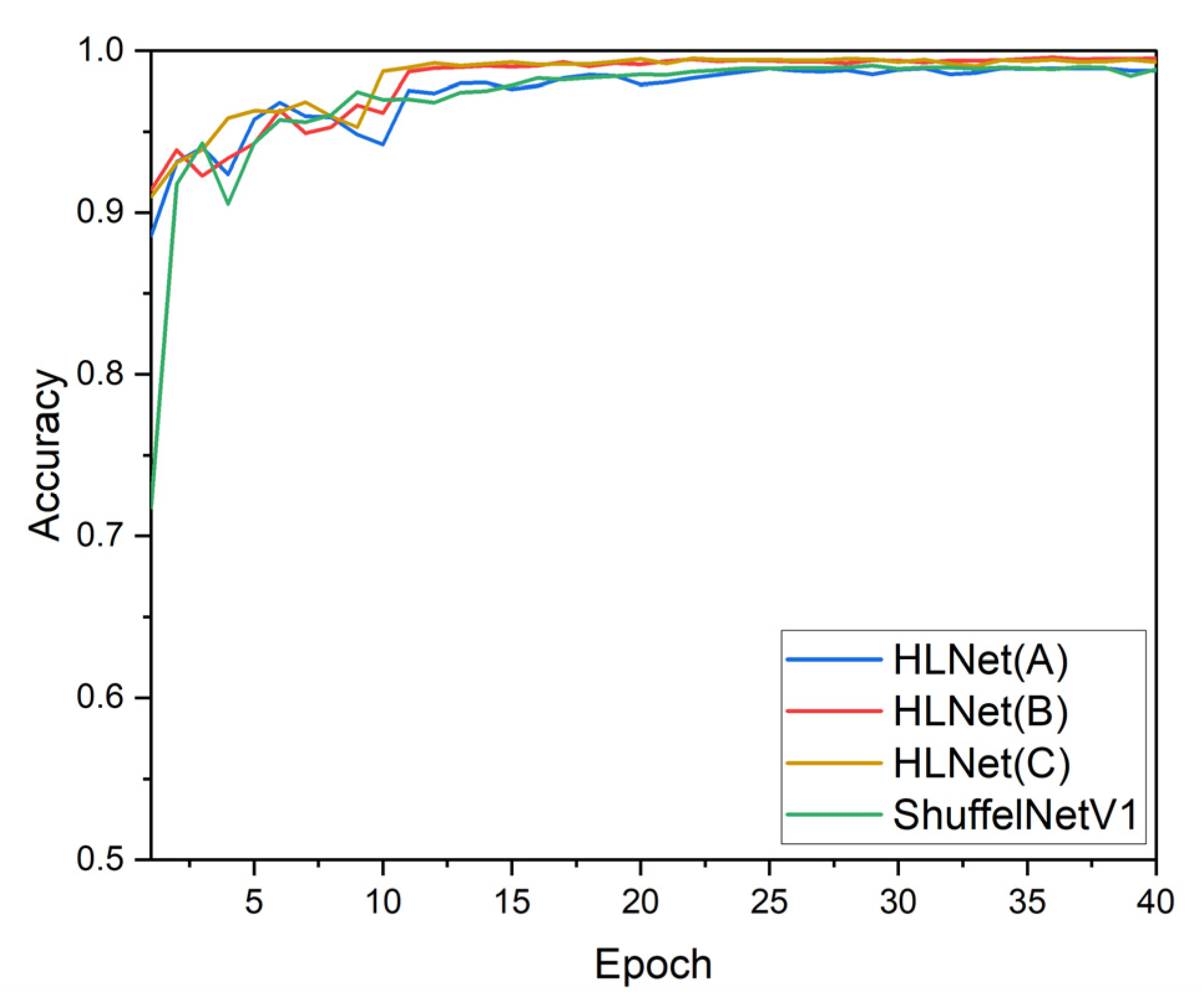
3.1. Improved ShuffleNetV1 Experimental Results and Analysis
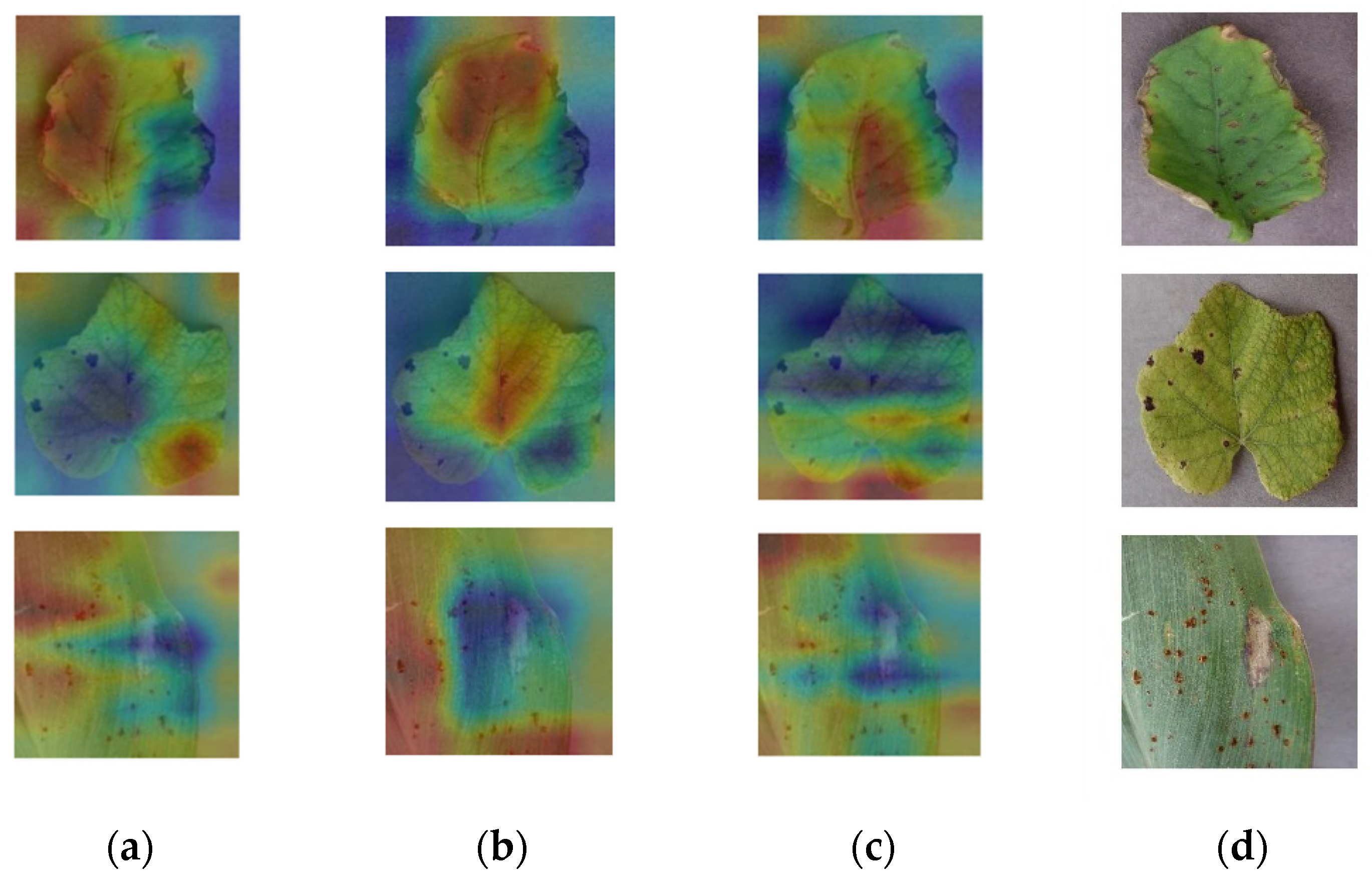
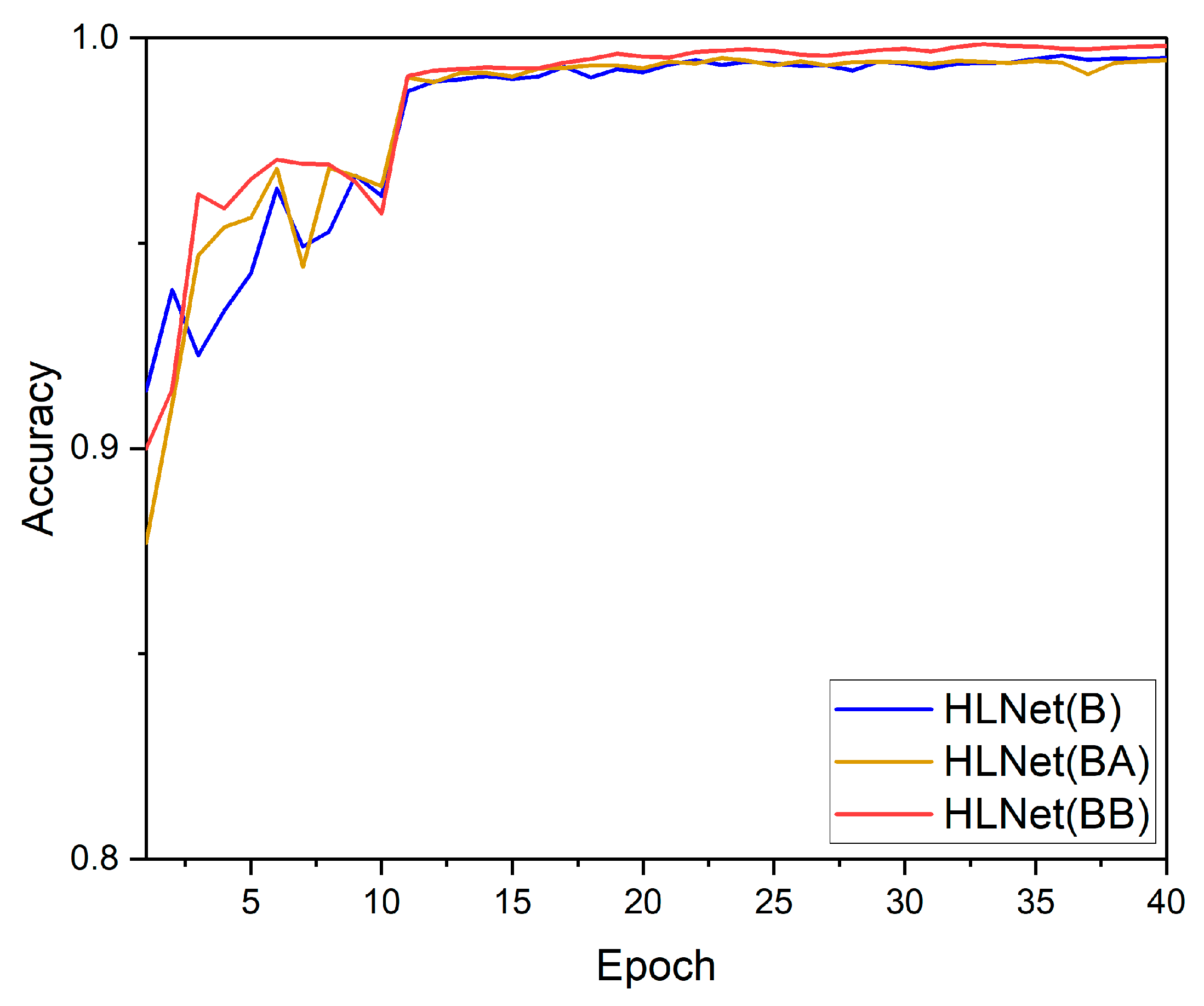
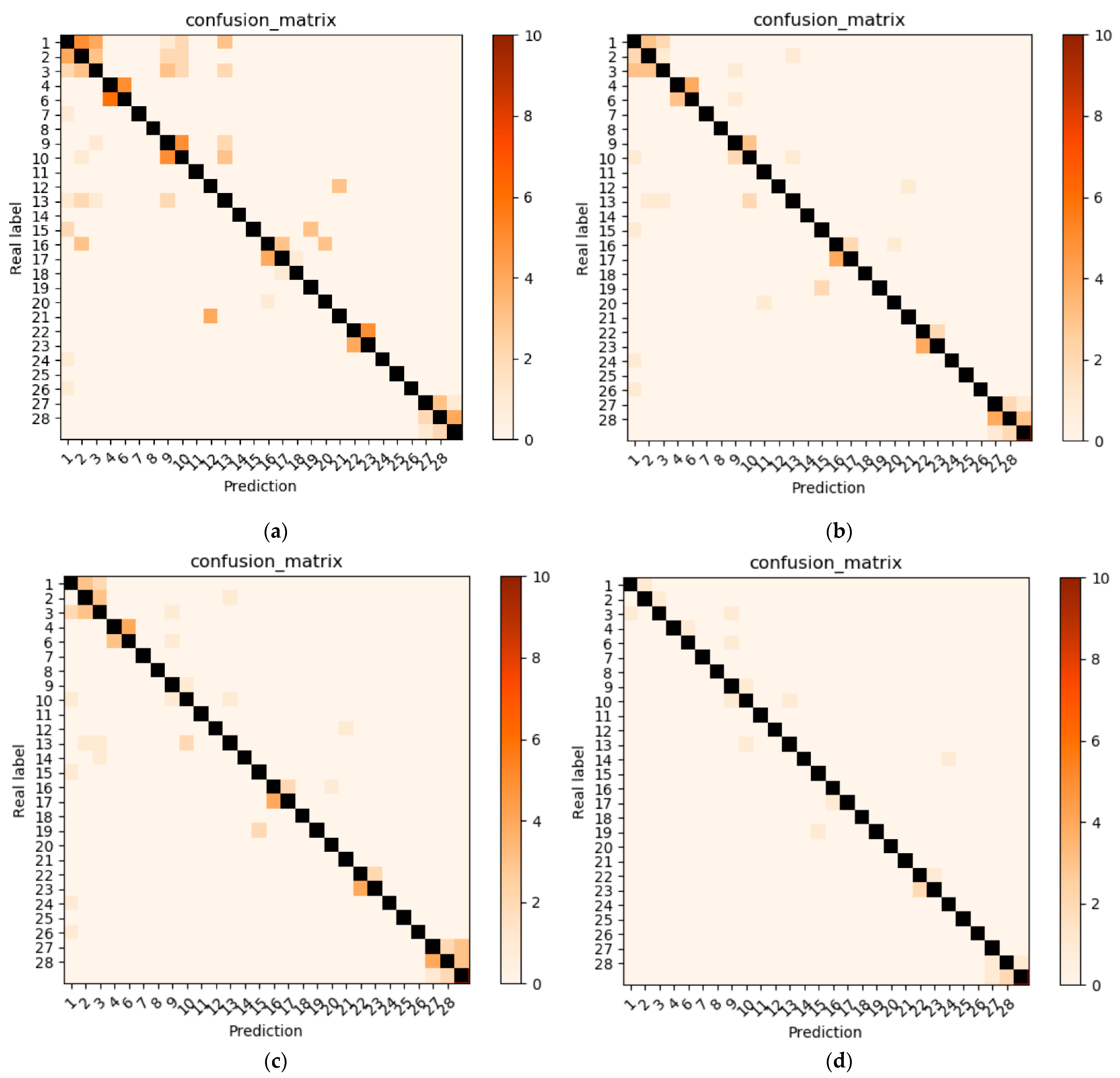
3.2. Attention Module Experimental Results and Analysis
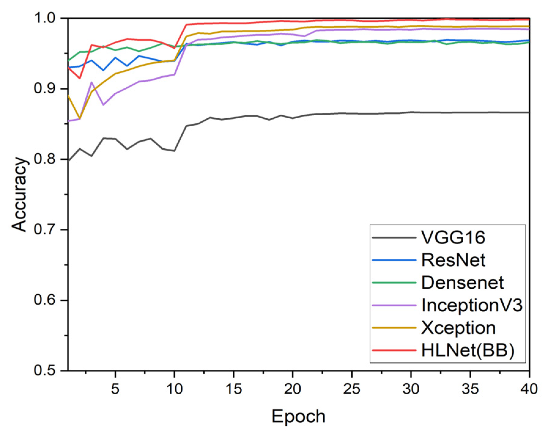
3.3. Comparison of Various Backbone Models
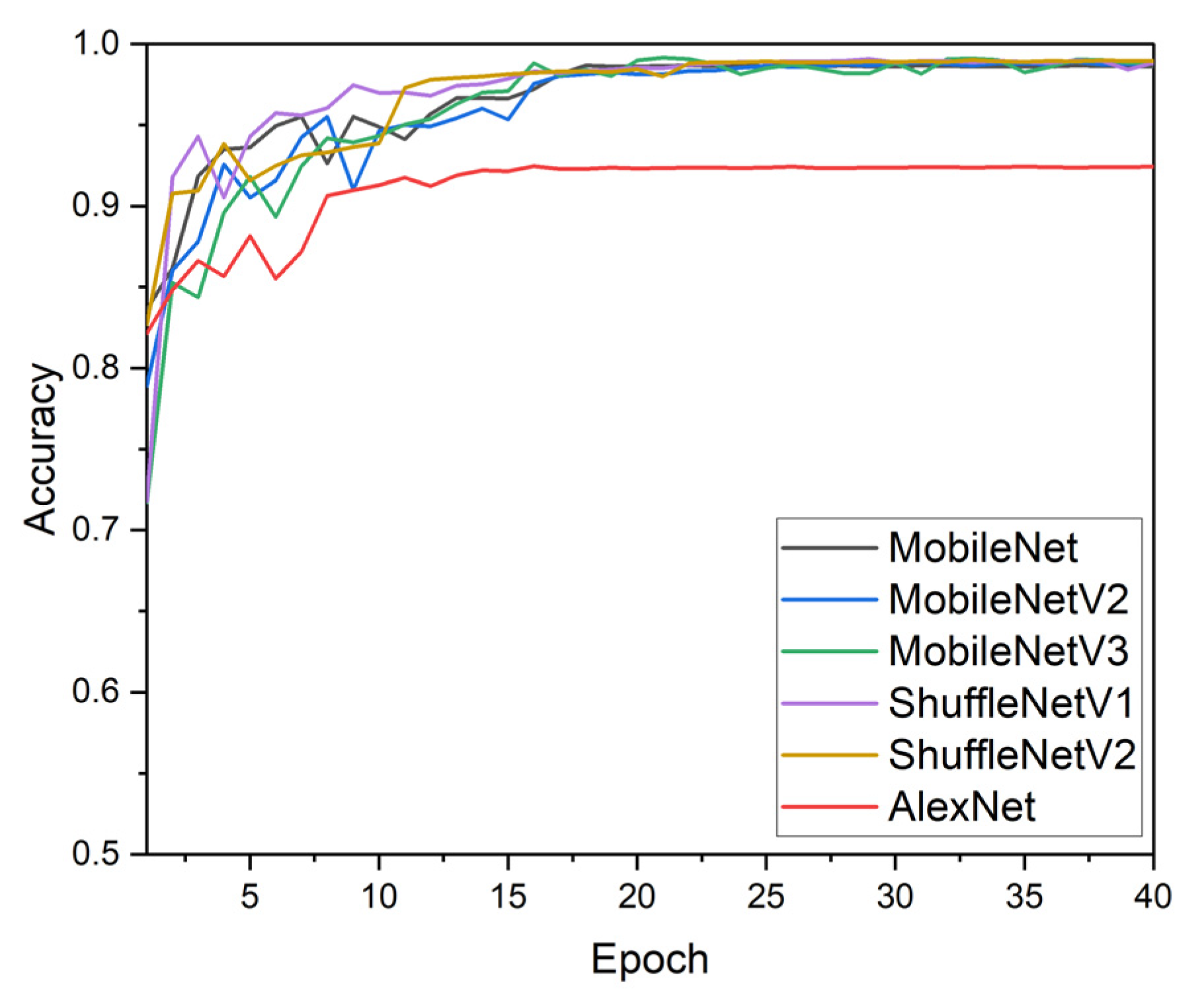
3.4. Comparison of Latest Lightweight Models
4. Conclusions
Author Contributions
Funding
Data Availability Statement
Conflicts of Interest
Appendix A

| Classes Num | Variety | Disease | Image Num |
|---|---|---|---|
| 1 | Apple | Apple_scab | 2016 |
| 2 | Black_rot | 1987 | |
| 3 | Cedar_apple_rust | 1760 | |
| 4 | Healthy | 2008 | |
| 5 | Corn | Gray_leaf_spot | 1642 |
| 6 | Common_rust | 1907 | |
| 7 | Northern_leaf_Blight | 1907 | |
| 8 | Healthy | 1859 | |
| 9 | Potato | Early_blight | 1939 |
| 10 | Late_blight | 1939 | |
| 11 | Healthy | 1824 | |
| 12 | Grape | Black_rot | 1888 |
| 13 | Black_Measles | 1920 | |
| 14 | Leaf_blight | 1722 | |
| 15 | Healthy | 1692 | |
| 16 | Tomato | Bacterial_spot | 1702 |
| 17 | Early_blight | 1920 | |
| 18 | Late_blight | 1851 | |
| 19 | Leaf_mold | 1882 | |
| 20 | Septoria_leaf_spot | 1745 | |
| 21 | Spider_mites | 1741 | |
| 22 | Target_Spot | 1827 | |
| 23 | Tomato_mosaic_virus | 1790 | |
| 24 | Yellow_Leaf_Curl_Virus | 1961 | |
| 25 | Healthy | 1920 | |
| 26 | Rice | Bacterial leaf blight | 1438 |
| 27 | Brown spot | 1072 | |
| 28 | Leaf smut | 1016 |
References
- Tilman, D.; Balzer, C.; Hill, J.; Befort, B.L. Global food demand and the sustainable intensification of agriculture. Proc. Natl. Acad. Sci. USA 2011, 108, 20260–20264. [Google Scholar] [CrossRef] [Green Version]
- Pantazi, X.E.; Moshou, D.; Tamouridou, A.A. Automated leaf disease detection in different crop species through image features analysis and One Class Classifiers. Comput. Electron. Agric. 2019, 156, 96–104. [Google Scholar] [CrossRef]
- Schwarzenbach, R.P.; Egli, T.; Hofstetter, T.B.; Von Gunten, U.; Wehrli, B. Global water pollution and human health. Annu. Rev. Environ. Resour. 2010, 35, 109–136. [Google Scholar] [CrossRef]
- Bock, C.H.; Poole, G.H.; Parker, P.E.; Gottwald, T.R. Plant disease severity estimated visually, by digital photography and image analysis, and by hyperspectral imaging. Crit. Rev. Plant Sci. 2010, 29, 59–107. [Google Scholar] [CrossRef]
- Ghosal, S.; Blystone, D.; Singh, A.K.; Ganapathysubramanian, B.; Singh, A.; Sarkar, S. An explainable deep machine vision framework for plant stress phenotyping. Proc. Natl. Acad. Sci. USA 2018, 115, 4613–4618. [Google Scholar] [CrossRef] [Green Version]
- Kumar, S.D.; Esakkirajan, S.; Bama, S.; Keerthiveena, B. A microcontroller based machine vision approach for tomato grading and sorting using SVM classifier. Microprocess. Microsyst. 2020, 76, 103090. [Google Scholar] [CrossRef]
- Goel, N.; Sehgal, P. Fuzzy classification of pre-harvest tomatoes for ripeness estimation—An approach based on automatic rule learning using decision tree. Appl. Soft Comput. 2015, 36, 45–56. [Google Scholar] [CrossRef]
- Ai, L.; Fang, N.F.; Zhang, B.; Shi, Z.H. Broad area mapping of monthly soil erosion risk using fuzzy decision tree approach: Integration of multi-source data within GIS. Int. J. Geogr. Inf. Sci. 2013, 27, 1251–1267. [Google Scholar] [CrossRef]
- Marconi, T.G.; Oh, S.; Ashapure, A.; Chang, A.; Jung, J.; Landivar, J.; Enciso, J. Application of unmanned aerial system for management of tomato cropping system. In Autonomous Air and Ground Sensing Systems for Agricultural Optimization and Phenotyping IV; International Society for Optics and Photonics: Bellingham, WA, USA, 2019; p. 11008. [Google Scholar] [CrossRef]
- Mohanty, S.P.; Hughes, D.P.; Salathé, M. Using deep learning for image-based plant disease detection. Front. Plant Sci. 2016, 7, 1419. [Google Scholar] [CrossRef] [Green Version]
- Zhang, X.; Qiao, Y.; Meng, F.; Fan, C.; Zhang, M. Identification of maize leaf diseases using improved deep convolutional neural networks. IEEE Access 2018, 6, 30370–30377. [Google Scholar] [CrossRef]
- Zhang, Y.; Wa, S.; Liu, Y.; Zhou, X.; Sun, P.; Ma, Q. High-Accuracy Detection of Maize Leaf Diseases CNN Based on Multi-Pathway Activation Function Module. Remote Sens. 2021, 13, 4218. [Google Scholar] [CrossRef]
- Liu, B.; Zhang, Y.; He, D.; Li, Y. Identification of apple leaf diseases based on deep convolutional neural networks. Symmetry 2018, 10, 11. [Google Scholar] [CrossRef] [Green Version]
- Deng, R.; Tao, M.; Xing, H.; Yang, X.; Liu, C.; Liao, K.; Qi, L. Automatic diagnosis of rice diseases using deep learning. Front. Plant. Sci. 2021, 12, 1691. [Google Scholar] [CrossRef]
- Oppenheim, D.; Shani, G.; Erlich, O.; Tsror, L. Using deep learning for image-based potato tuber disease detection. Phytopathology 2019, 109, 1083–1087. [Google Scholar] [CrossRef]
- Iandola, F.N.; Han, S.; Moskewicz, M.W.; Ashraf, K.; Dally, W.J.; Keutzer, K. SqueezeNet: AlexNet-level accuracy with 50x fewer parameters and <0.5 MB model size. arXiv 2016, arXiv:1602.07360. [Google Scholar]
- Howard, A.G.; Zhu, M.; Chen, B.; Kalenichenko, D.; Wang, W.; Weyand, T.; Adam, H. Mobilenets: Efficient convolutional neural networks for mobile vision applications. arXiv 2017, arXiv:1704.04861. [Google Scholar]
- Chollet, F. Xception: Deep learning with depthwise separable convolutions. In Proceedings of the IEEE Conference on Computer Vision and Pattern Detection (CVPR), Honolulu, HI, USA, 22–25 July 2017; pp. 1251–1258. [Google Scholar]
- Zhang, X.; Zhou, X.; Lin, M.; Sun, J. Shufflenet: An extremely efficient convolutional neural network for mobile devices. In Proceedings of the CVPR, Salt Lake City, UT, USA, 18–22 June 2018; pp. 5848–6856. [Google Scholar]
- Kamal, K.C.; Yin, Z.; Wu, M.; Wu, Z.L. Depthwise separable convolution architectures for plant disease classification. Comput. Electron. Agric. 2019, 165, 104948. [Google Scholar] [CrossRef]
- Wagle, S.A.; Harikrishnan, R.; Ali, S.H.M.; Faseehuddin, M. Classification of plant leaves using new compact convolutional neural network models. Plants 2022, 11, 24. [Google Scholar] [CrossRef]
- Wang, P.; Niu, T.; Mao, Y.R.; Liu, B.; Yang, S.Q.; He, D.J.; Gao, Q. Fine-Grained Grape Leaf Diseases Recognition Method Based on Improved Lightweight Attention Network. Front. Plant. Sci. 2021, 12, 738042. [Google Scholar] [CrossRef]
- Bi, C.K.; Wang, J.M.; Duan, Y.L.; Fu, B.F.; Kang, J.R.; Shi, Y. MobileNet Based Apple Leaf Diseases Identification. Mob. Netw. Appl. 2022, 27, 172–180. [Google Scholar] [CrossRef]
- Bhujel, A.; Kim, N.E.; Arulmozhi, E.; Basak, J.K.; Kim, H.T. A lightweight Attention-based convolutional neural networks for tomato leaf disease classification. Agriculture 2022, 12, 228. [Google Scholar] [CrossRef]
- Chao, X.F.; Hu, X.; Feng, J.Z.; Zhang, Z.; Wang, M.L.; He, D.J. Construction of apple leaf diseases identification networks based on xception fused by SE module. Appl. Sci. 2021, 11, 14. [Google Scholar] [CrossRef]
- Hughes, D.; Salathé, M. An open access repository of images on plant health to enable the development of mobile disease diagnostics. arXiv 2015, arXiv:1511.08060. [Google Scholar]
- UC Irvine Machine Learning Repository. Available online: https://archive.ics.uci.edu/ml/datasets/Rice+Leaf+Diseases (accessed on 14 April 2019).
- Peng, D.; Zhang, Y.; Guan, H. End-to-end change detection for high resolution satellite images using improved UNet++. Remote Sens. 2019, 11, 1382. [Google Scholar] [CrossRef] [Green Version]
- Xu, G.; Liu, M.; Jiang, Z.; Söffker, D.; Shen, W. Bearing fault diagnosis method based on deep convolutional neural network and random forest ensemble learning. Sensors 2019, 19, 1088. [Google Scholar] [CrossRef] [PubMed] [Green Version]
- Shujaat, M.; Wahab, A.; Tayara, H.; Chong, K.T. pcPromoter-CNN: A CNN-Based Prediction and Classification of Promoters. Genes 2020, 11, 1529. [Google Scholar] [CrossRef] [PubMed]
- Tian, C.; Zhuge, R.; Wu, Z.; Xu, Y.; Zuo, W.; Chen, C.; Lin, C.W. Lightweight image super-resolution with enhanced CNN. Knowl. Based Syst. 2020, 205, 106235. [Google Scholar] [CrossRef]
- Hu, J.; Shen, L.; Sun, G. Squeeze-and-excitation networks. In Proceedings of the CVPR, Salt Lake City, UT, USA, 18–22 June 2018; pp. 7132–7141. [Google Scholar]
- Woo, S.; Park, J.; Lee, J.Y.; Kweon, I.S. Cbam: Convolutional block attention module. In Proceedings of the European Conference on Computer Vision (ECCV), Munich, Germany, 8–14 September 2018; pp. 3–19. [Google Scholar]
- Kingma, D.P.; Ba, J. Adam: A method for stochastic optimization. arXiv 2014, arXiv:1412.6980. [Google Scholar]
- Zhou, B.; Khosla, A.; Lapedriza, A.; Oliva, A.; Torralba, A. Learning deep features for discriminative localization. In Proceedings of the CVPR, Las Vegas, NV, USA, 27–30 June 2016; pp. 2921–2929. [Google Scholar]
- Simonyan, K.; Zisserman, A. Very deep convolutional networks for large-scale image detection. arXiv 2014, arXiv:1409.1556. [Google Scholar]
- He, K.; Zhang, X.; Ren, S.; Sun, J. Deep residual learning for image detection. In Proceedings of the CVPR, Las Vegas, NV, USA, 27–30 June 2016; pp. 770–778. [Google Scholar]
- Huang, G.; Liu, Z.; Van Der Maaten, L.; Weinberger, K.Q. Densely connected convolutional networks. In Proceedings of the CVPR, Honolulu, HI, USA, 22–25 July 2017; pp. 4700–4708. [Google Scholar]
- Szegedy, C.; Vanhoucke, V.; Ioffe, S.; Shlens, J.; Wojna, Z. Rethinking the inception architecture for computer vision. In Proceedings of the CVPR, Las Vegas, NV, USA, 27–30 June 2016; pp. 2818–2826. [Google Scholar]
- Krizhevsky, A.; Sutskever, I.; Hinton, G.E. Imagenet classification with deep convolutional neural networks. Adv. Neural Inf. Processing Syst. 2012, 25, 1097–1105. [Google Scholar] [CrossRef]
- Sandler, M.; Howard, A.; Zhu, M.; Zhmoginov, A.; Chen, L.C. Mobilenetv2: Inverted residuals and linear bottlenecks. In Proceedings of the CVPR, Salt Lake City, UT, USA, 18–22 June 2018; pp. 4510–4520. [Google Scholar]
- Howard, A.; Sandler, M.; Chu, G.; Chen, L.-C.; Chen, B.; Tan, M.; Wang, W.; Zhu, Y.; Pang, R.; Vasudevan, V.; et al. Searching for mobilenetv3. In Proceedings of the ICCV, Seoul, Korea, 27 October–2 November 2019; pp. 1314–1324. [Google Scholar]
- Ma, N.; Zhang, X.; Zheng, H.T.; Sun, J. Shufflenet v2: Practical guidelines for efficient cnn architecture design. In Proceedings of the ECCV, Munich, Germany, 8–14 September 2018; pp. 116–131. [Google Scholar]
- Deng, J.; Dong, W.; Socher, R.; Li, L.J.; Li, K.; Fei-Fei, L. Imagenet: A large-scale hierarchical image database. In Proceedings of the CVPR, Miami Beach, FL, USA, 20–24 June 2009; pp. 248–255. [Google Scholar]

| Layer | Input Size | Output Size | Repeat | Stride | Remarks |
|---|---|---|---|---|---|
| Image | 224 × 224 × 3 | 224 × 224 × 3 | |||
| Conv 1 Conv 2 | 224 × 224 × 3 224 × 224 × 3 | 112 × 112 × 12 112 × 112 × 12 | 1 1 | 2 2 | |
| Stage 0 | 112 × 112 × 24 | 56 × 56 × 48 | 1 | 2 | |
| Stage 1 | 56 × 56 × 48 | 56 × 56 × 72 | 2 | 1 | |
| Stage 2 | 56 × 56 × 72 | 28 × 28 × 144 | 1 3 | 2 1 | |
| Stage 3 | 28 × 28 × 144 | 14 × 14 × 288 | 1 3 | 2 1 | |
| Stage 4 | 14 × 14 × 288 | 7 × 7 × 576 | 1 3 | 2 1 | Join Att |
| Stage 5 | 7 × 7 × 576 | 7 × 7 × 1152 | 2 | 1 | Join Att |
| AdaptiveAvgPool | 7 × 7 × 1152 | 1 × 1 × 1152 | |||
| FC | 1 × 1 × 1152 | 28 |
| Name | Num |
|---|---|
| Adam learning rate Weight decay | 1 × 10⁻³ 0.001 |
| Epoch | 40 |
| Batch size | 10 |
| Image size | 224 × 224 |
| Group | 3 |
| Classes | 28 |
| Name | Best Acc (%) | FLOPs (M) | Model Size (K) | Computation Time (s) |
|---|---|---|---|---|
| HLNet (A) | 98.98 | 200.59 | 6375 | 0.166 |
| HLNet (B) | 99.56 | 200.59 | 6375 | 0.166 |
| HLNet (C) | 99.46 | 200.59 | 6375 | 0.166 |
| ShuffleNetV1 | 99.00 | 579.5 | 6891 | 0.236 |
| Name | Best Acc (%) | FLOPs (M) | Model Size (K) | Computation Time (s) |
|---|---|---|---|---|
| HLNet (B) | 99.56 | 200.59 | 6375 | 0.166 |
| HLNet (BA) | 99.58 | 264.15 | 9096 | 0.208 |
| HLNet (BB) | 99.86 | 248.07 | 8239 | 0.173 |
| Name | Best Acc (%) | FLOPs (M) | Model Size (K) | Computation Time (s) |
|---|---|---|---|---|
| HLNet (BB) | 99.86 | 238.44 | 8235 | 0.173 |
| AlexNet | 92.40 | 715.54 | 238,690 | 0.182 |
| VGG16 | 86.62 | 15.5 × 1024 | 540,463 | 0.255 |
| ResNet101 | 96.92 | 7.84 × 1024 | 100,100 | 0.389 |
| DenseNet161 | 96.89 | 7.82 × 1024 | 113,019 | 0.562 |
| MobileNet | 98.70 | 581.7 | 8261 | 0.187 |
| MobileNetV2 | 98.90 | 318.99 | 7353 | 0.210 |
| MobileNetV3 | 98.96 | 265.15 | 10,833 | 0.312 |
| ShuffleNetV1 | 99.00 | 579.5 | 6891 | 0.236 |
| ShuffleNetV2 | 98.96 | 198.73 | 9003 | 0.198 |
| SqueezeNet | 41.92 | 355.69 | 4850 | 0.149 |
| InceptionV3 | 98.91 | 2.85 × 1024 | 95,748 | 0.293 |
| Xception | 98.89 | 4.58 × 1024 | 81,808 | 0.306 |
| Name | Crop Number | Years | Model | Best ACC (%) | Flops (M) | Model Size (K) | Computation Time (s) |
|---|---|---|---|---|---|---|---|
| Our study | 6 | 2022 | HLNet (B) | 99.56 | 200.59 | 6375 | 0.166 |
| HLNet (BB) | 99.86 | 238.44 | 8235 | 0.173 | |||
| N1 model | 99.45 | - | 15,155 | - | |||
| Wagle, S. A. et al. [21] | 9 | 2021 | N2 model | 99.65 | - | 30,412 | - |
| N3 model | 99.55 | - | 15,155 | - | |||
| Wang, P. et al. [22] | 1 | 2021 | ECA-SNett_0.5× | 98.86 | 37.4 | - | - |
| ECA-SNett_1.0× | 99.66 | 125.6 | - | - | |||
| lw_resnet20 | 98.85 | 499.5 | 16,998 | 0.795 | |||
| lw_resnet20_cbam | 99.69 | 450.56 | 17,203 | 0.914 | |||
| Bhujel, A. et al. [24] | 1 | 2022 | lw_resnet20_se | 98.85 | 450.56 | 17,203 | 0.927 |
| lw_resnet20_sa | 99.32 | 566.27 | 18,739 | 0.961 | |||
| lw_resnet20_da | 98.90 | 601.09 | 18,022 | 0.984 | |||
| Chao, X. et al. [25] | 1 | 2021 | SE_Xception | 99.40 | 48.15 | - | - |
| SE_miniXception | 97.01 | 6.67 | - | - |
Publisher’s Note: MDPI stays neutral with regard to jurisdictional claims in published maps and institutional affiliations. |
© 2022 by the authors. Licensee MDPI, Basel, Switzerland. This article is an open access article distributed under the terms and conditions of the Creative Commons Attribution (CC BY) license (https://creativecommons.org/licenses/by/4.0/).
Share and Cite
Xu, Y.; Kong, S.; Gao, Z.; Chen, Q.; Jiao, Y.; Li, C. HLNet Model and Application in Crop Leaf Diseases Identification. Sustainability 2022, 14, 8915. https://doi.org/10.3390/su14148915
Xu Y, Kong S, Gao Z, Chen Q, Jiao Y, Li C. HLNet Model and Application in Crop Leaf Diseases Identification. Sustainability. 2022; 14(14):8915. https://doi.org/10.3390/su14148915
Chicago/Turabian StyleXu, Yanlei, Shuolin Kong, Zongmei Gao, Qingyuan Chen, Yubin Jiao, and Chenxiao Li. 2022. "HLNet Model and Application in Crop Leaf Diseases Identification" Sustainability 14, no. 14: 8915. https://doi.org/10.3390/su14148915
APA StyleXu, Y., Kong, S., Gao, Z., Chen, Q., Jiao, Y., & Li, C. (2022). HLNet Model and Application in Crop Leaf Diseases Identification. Sustainability, 14(14), 8915. https://doi.org/10.3390/su14148915