Article

The Spatial Spillover Effects of Environmental Regulation and Regional Energy Efficiency and Their Interactions under Local Government Competition in China

School of Mathematics and Statistics, Fujian Normal University, Fuzhou 350117, China
*
Author to whom correspondence should be addressed.
Sustainability 2022, 14(14), 8753; https://doi.org/10.3390/su14148753
Submission received: 9 June 2022 / Revised: 11 July 2022 / Accepted: 15 July 2022 / Published: 18 July 2022
(This article belongs to the Topic Climate Change and Environmental Sustainability)

Abstract

:
Under the pressure of serious environmental pollution and energy shortage, China needs to improve its energy efficiency to alleviate these problems. Environmental regulation is an important constraint on economic development, which has an impact on energy efficiency. Meanwhile, energy efficiency is a reference factor for adjusting environmental policies, which has an impact on environmental regulation. Therefore, the relationship between environmental regulation and energy efficiency needs to be further studied under a unified framework. Based on Chinese provincial panel data, we first use a stochastic frontier model to estimate the energy efficiency of China’s 30 provinces from 2004 to 2019, and then employ a spatial simultaneous equation model to study the spatial spillover effects of environmental regulation and energy efficiency and their interactions. The results show that: (1) Both energy efficiency and environmental regulation have significantly positive spatial spillover effects. Specifically, an overall increase of 1% in energy efficiency in the surrounding areas can promote an improvement in the local energy efficiency by about 1.0404%, and an overall increase of 1% in environmental regulation in the surrounding areas can lead to an increase of about 0.6075% in the local environmental regulation. (2) The impact of environmental regulation on energy efficiency is significantly positive; i.e., under the current situation in China, an increase of 1% in environmental regulation can promote local energy efficiency by about 0.2777%. (3) The impact of energy efficiency on environmental regulation is significantly positive; i.e., a 1% increase in energy efficiency may stimulate local governments to strengthen their environmental regulation by 1.5981%. Accordingly, some targeted policy suggestions are given.

1. Introduction

With the continuous progress of environmental degradation and climate change in recent decades, environmental sustainability has become one of the most concerning issues in the world [1]. Emissions from energy consumption are the root cause of environmental problems [2]. Therefore, improving energy efficiency is a feasible way to reduce fossil fuel consumption [3,4,5]. Environmental regulation forms an important constraint on energy efficiency [6,7,8]. So, effective environmental regulation is helpful to solve the problem of environmental sustainability. An in-depth study of environmental regulation and energy efficiency will help to find more effective environmental regulation policies and contribute to environmental sustainability.
Since the reform and opening up of China, its economy has achieved great development. However, China’s energy consumption has soared in the past decades [9]. According to the data from the International Energy Agency, China has been the world’s largest energy user since 2009. In 2019, China’s total energy consumption reached 143.92 exajoules, accounting for 24.5% of the world’s total consumption (Accessed from: https://www.bp.com/content/dam/bp/business-sites/en/global/corporate/xlsx/energy-economics/statistical-review/bp-stats-review-2022-all-data.xlsx (accessed on 1 June 2022)). However, China’s GDP was only 16.35% of the world’s total GDP in 2019. This shows that China’s energy efficiency is low and there is still considerable room for improvement. China’s massive energy consumption has brought serious environmental pollution. According to the China Ecological and Environmental Bulletin (2019), about 53.4% of China’s cities exceeded the air pollution standards, acid rain covered an area of 474,000 square kilometers, the proportion of the inferior V class of the national surface water was 3.4%, and the proportion of substandard drinking water sources in use was as high as 8.0% (Accessed from: http://www.mee.gov.cn/hjzl/sthjzk/zghjzkgb/202006/P020200602509464172096.pdf (accessed on 1 June 2022)).
In recent years, the haze has seriously affected people’s normal life. Therefore, environmental protection has become an important topic in China. A large part of the pollution problems in the world is caused by energy consumption [2]. However, human life and economic development cannot be separated from energy consumption. How, then, does one achieve sustainable economic development while reducing environmental pollution? One way is to replace traditional energy with clean energy, such as wind energy, water energy, solar energy, and nuclear energy, and another is to improve energy efficiency [10]. The prospect of replacing traditional energy with clean energy is certainly good, and most countries in the world are investing heavily in this field. However, due to the limited progress of energy technologies, there are considerable uncertainties in the short term. Improving energy efficiency has great potential and is feasible in both the short and long term [11].
As the world’s largest energy consumer, improving energy efficiency will not only alleviate China’s energy shortage and improve its environmental quality, but also help save world energy and contribute to world environmental development [12]. Therefore, it is necessary to study China’s energy efficiency. In China, the government influences almost every aspect of household and business activities, so the study of energy efficiency cannot be separated from environmental regulation of the Chinese government [13].
Environmental regulation affects residents’ energy consumption. Moreover, it also has important constraints on the production technology, energy input, and energy structure adopted by enterprises, thus affecting the energy efficiency of the region [7,11]. At the same time, the change in local energy efficiency is an important factor for the government to adjust the environmental regulation policies. Therefore, it is one-sided to only study the impact of environmental regulation on energy efficiency, and it is necessary to discuss their interactive effects. Meanwhile, due to the political system of “promotion tournament” in China, local governments compete for economic development [14]. It is a conventional means to attract investment to boost economic growth by adjusting the intensity of environmental regulation, so the environmental regulation of a region is naturally affected by the environmental regulation policies of neighboring regions [15,16,17]. Moreover, due to technology spillover and resource flow, the energy efficiency of this region is also affected by the energy efficiency of neighboring regions; that is, energy efficiency has the feature of spatial agglomeration [8,9].
Therefore, unlike the previous literature that only studied the impact of environmental regulation on energy efficiency, the goal of this paper is to study the interactions between energy efficiency and environmental regulation and their spatial spillover effects under a unified framework. Besides that, we will try to reveal the performance pattern of China’s environmental regulation from the perspective of local government competition.
The rest of this paper is organized as follows. We briefly review the related literature in Section 2. Section 3 analyzes the mechanism of environmental regulation and energy efficiency. Section 4 presents the empirical data and provides a measurement of energy efficiency. Section 5 describes the empirical model. Section 6 reports the empirical results and then discusses the results. In the final section we offer some policy implications.

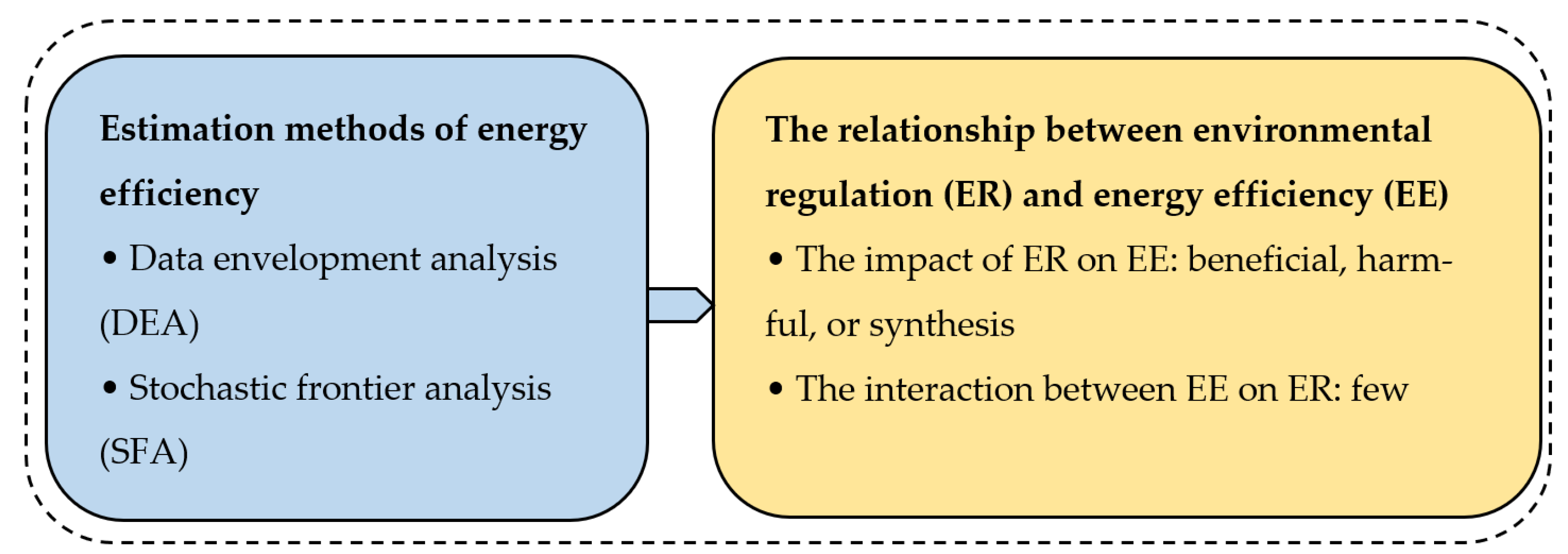
2. Literature Review

The research related to this paper includes the estimation of energy efficiency as well as empirical research on the relationship between environmental regulation and energy efficiency. Therefore, we will review the literature from these two aspects. The overview of relevant literature is shown in Figure 1.
An objective evaluation of energy efficiency is the key to study energy efficiency. Currently, the methods to estimate energy efficiency mainly include data envelopment analysis (DEA) and stochastic frontier analysis (SFA). Data envelopment analysis (DEA) is a non-parametric method, which has the advantages of extensibility and easy operation, so it has received a lot of attention and application. Zhao et al. [10] used the three-stage data envelopment analysis model to estimate China’s energy efficiency between 2008 and 2016. Lu et al. [18] used the dynamic data envelopment analysis model to evaluate the energy efficiency of European Union countries during the period 2009–2013. Rakshit and Mandal [19] conducted a more extensive empirical study using the DEA method to estimate energy efficiency in low-income, middle-income, and high-income economies from 1993 to 2013. There were other scholars who also had made meaningful studies with the DEA method [20,21,22,23].
However, the energy efficiency estimated by the DEA method is the relative efficiency of an intra-group sample comparison, which is extremely sensitive to the possible abnormal samples in the data set [24]. Moreover, the usual DEA method is to estimate the cross-sectional samples, and the estimated energy efficiency is often not comparable between different years. In view of the disadvantages of DEA, we will use the panel data stochastic frontier model to estimate energy efficiency. The main reason is that the stochastic frontier model takes the disturbance of random factors into consideration when determining the efficiency frontier. The estimation results are more robust; in addition, the panel data stochastic frontier model can effectively solve the problem of comparability of estimation results at different times [25].
The stochastic frontier model was proposed by Aigner et al. [26], Battese et al. [27], and Meeusen et al. [28], and subsequently improved by other scholars [29,30,31]. It has been widely used in efficiency estimation. Al-Gasaymeh [32] used SFA to estimate bank efficiency in the Gulf Cooperation Council countries. Ferreira and Feres [33] employed SFA to estimate land-use efficiency in the Brazilian Amazon. Miao et al. [34] also used SFA when studying the technological innovation efficiency of Chinese industrial enterprises. These studies yielded some meaningful results.
At present, there are few studies on the interaction between environmental regulation and energy efficiency, while there are many on the impact of environmental regulation on energy efficiency. Therefore, we mainly review the impact of environmental regulation on energy efficiency.
Empirical evidence shows that environmental regulation has different effects on the energy efficiency of different countries or regions and different industries. Mandal [35] used DEA to measure the energy efficiency of the cement industry in India. The empirical results showed that environmental regulation enhanced the energy efficiency. The study of Bi et al. [36] showed environmental regulation had a positive effect on the energy efficiency of China’s thermal power plants. Kneller and Manderson [37] showed that environmental regulation could promote environmental investment of British enterprises, but there was no evidence that environmental regulation stimulated R&D activities. Wang and Du [38] and Zhang et al. [39], respectively, used the extended directional distance function and super-efficiency DEA model to estimate China’s provincial energy efficiency, and the subsequent empirical studies showed that China’s environmental regulation promoted an improvement in energy efficiency. Pan et al. [40] used a directed acyclic graph to study the dynamic relationship between environmental regulation and regional energy efficiency and found that both market-driven environmental regulation and mandatory environmental regulation were beneficial to energy efficiency.
Barbera and McConnell [41] and Jorgenson and Wilcoxen [42] proposed that environmental regulation could increase the “compliance cost” of enterprises and force enterprises to change the optimal production decisions, thereby reducing the energy efficiency of enterprises. Lanoie’s empirical study of Quebec’s manufacturing sector supports the above hypothesis [43]. Wang et al. [44] found that China’s command–control and economic incentive environmental regulations inhibit energy efficiency.
Many scholars believe that the impact of environmental regulation on energy efficiency is complex and uncertain. This view is the synthesis of the above two theories. Lin and Xu [11] adopted a slacks-based measure (SBM)-undesirable model to calculate the inter-provincial energy efficiency in China, and used a Tobit panel regression model to study the effect of environmental regulation on energy efficiency. The results showed that environmental regulation forced the eastern region to reduce the proportion of fossil energy and increase the proportion of clean energy, so as to improve the energy efficiency, but the energy efficiency in the west declined due to preemptive energy extraction. Li et al. [6] measured the energy efficiency of Xi’an city with the DEA method; they found that environmental regulation had no effect on energy efficiency. Zhu et al. [8] divided environmental regulation into voluntary environmental regulation and mandatory environmental regulation. Based on a spatial econometric model, they concluded that voluntary environmental regulation had a positive impact on energy efficiency, while mandatory environmental regulation had no significant effect on energy efficiency. However, it remains puzzling that even studies of the effects of environmental regulation on energy efficiency in the same region have yielded considerable deviations. Yu et al. [45] used the panel dynamic spatial econometric model to study the impact of environmental regulation on energy efficiency. The results showed that China’s environmental regulation reduced emissions but did not improve energy efficiency. Peng [46], however, confirmed that China’s environmental regulation was conducive to improving energy efficiency. The studies of Gao and You [47] and Li et al. [48] showed that there was a “U-shaped” relationship between environmental regulation and energy efficiency in China. In other words, the weak intensity of environmental regulation was not conducive to an improvement in energy efficiency, but it could promote an improvement in energy efficiency after the environmental regulation intensity crossed a certain “inflection point”.
To sum up, there are still some areas that can be improved. (1) In the past, the literatures on the impact of environmental regulation on energy efficiency mostly adopt the single equation model, setting environmental regulation as exogenous; however, this is not the case in reality. Environmental regulation and energy efficiency are often interrelated, so it is necessary to establish a simultaneous equation model to consider their mutual influence mechanism. (2) Energy efficiency has a spatial spillover effect due to resource flow and technology spillover. As the environmental policies of local governments in China are evolving in competition, environmental regulation also has a spatial spillover effect. Therefore, it is necessary to use a spatial econometric model to study the spatial spillover effects of energy efficiency and environmental regulation. On the basis of previous research, this paper will use the spatial simultaneous equation model to carry out the research.

3. Mechanism Analysis on Environmental Regulation and Energy Efficiency

Before the empirical test, we need to analyze the theoretical mechanism of the interaction between environmental regulation and energy efficiency. The theoretical mechanism of their spatial spillover effects also needs to be analyzed.
There are three representative views on the impact of environmental regulation on energy efficiency. The first view is that environmental regulation is detrimental to energy efficiency, as its logic is the “compliance cost hypothesis”. Due to environmental regulations, enterprises have to invest to control environmental pollution and pay pollution fees. The increase in costs may squeeze enterprises’ investment in energy utilization [41,42], which could lead to a decline in energy efficiency. In addition, some scholars proposed a “green paradox”. Energy producers expect the government to strengthen environmental regulations in the future, so they exploit more energy at present and sell it at a lower price. This stimulates enterprises to consume more energy, which leads to a lower energy efficiency [49]. The second view holds that proper environmental regulations can force enterprises to innovate in energy technology and improve the energy management level, which can even cover compliance costs and improve energy efficiency [50]. In addition, environmental regulation may influence household energy consumption preferences, thus enabling households to save energy and improve energy efficiency. The third view is a synthesis of the above two; it holds that environmental regulation may not only reduce energy efficiency due to the compliance cost effect and “green paradox”, but also improve energy efficiency due to the innovation compensation effect. Therefore, the comprehensive effect is uncertain and depended on which of the above two influences is dominant [7,11]. From the above analysis, it can be seen that the impact mechanism of environmental regulation on energy efficiency is relatively complex. In different regions and different development stages, environmental regulation may affect energy efficiency through different ways, and its overall effect may be positive or negative.
There are few studies on the reverse impact of energy efficiency on environmental regulation, but the impact may exist objectively. Environmental improvement is the goal of local government’s environmental regulation and also an important reference factor for its adjustment of environmental regulation policy. However, it is worth noting that economic growth is the first goal pursued by most countries. People are willing to accept improving the environment on the basis of economic growth. Economic growth is inseparable from power, which usually comes from energy consumption. Therefore, under the constraints of economic growth, improving energy efficiency has become an inevitable choice to improve environmental quality. Therefore, energy efficiency affects environmental regulation by affecting environmental quality. Specifically, the improvement in energy efficiency contributes to the improvement in environmental quality under the premise of economic growth. After the improvement in environmental quality, local governments may continue to strengthen environmental regulation, or weaken environmental regulation because the environmental quality meets the standard. Therefore, the effect of energy efficiency on environmental regulation may be positive or negative.
People in high-income areas have higher requirements for environmental quality, which may lead to higher environmental regulation intensity in these areas. This is not friendly to enterprises with high pollution and energy consumption. In order to develop an economy and attract investment, the adjacent low-income areas tend to maintain a low intensity of environmental regulation and undertake investment from high-income areas. However, in order to retain investment, high-income areas may reduce the intensity of their environmental regulation. This, in turn, may stimulate the surrounding low-income areas to further reduce the intensity of their environmental regulation [15,16,17]. In China, due to the top–down political system, the promotion of lower-level officials is mainly determined by the higher-level officials according to certain criteria (similar to KPI). The assessment standard is mainly the local economic growth rate [14]. Because investment can significantly stimulate economic growth in the short term, most local government officials in China focus on attracting investment, and even lower environmental standards in exchange for enterprise investment when necessary. Therefore, the environmental regulation of a region will naturally be affected by the environmental regulation policies of neighboring regions [51]. Specifically, the intensity of environmental regulation in the region and its surrounding areas may change in the same direction.
Most industries are close to their supporting industries, while similar industries are synergistic. At the same time, there may be technology spillover and talent flow in adjacent areas. Therefore, the energy efficiency of a region will be affected by the energy efficiency of adjacent regions; that is, energy efficiency may have the characteristics of spatial agglomeration [8,9].

4. Data and Measures

4.1. Data Sources

The data used in this paper are the provincial data of 30 provinces in Chinese Mainland from 2003 to 2019. Due to a lack of data, Tibet is not included. All data are from the official website of the National Bureau of Statistics of China, and from the Provincial Statistical Yearbooks of each province (2004~2020), China Statistical Yearbook (2004~2020), China Environmental Yearbook (2005~2020), and China Energy Statistical Yearbook (2004~2020). All nominal economic indicators are adjusted based on 2004.

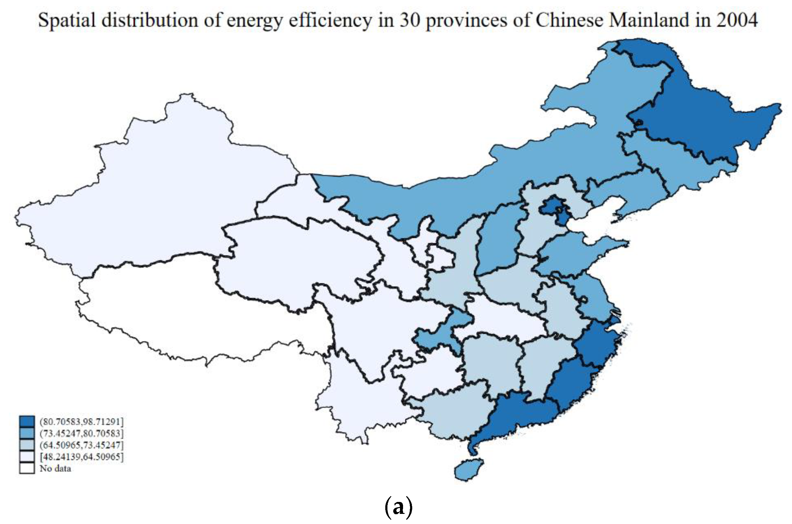
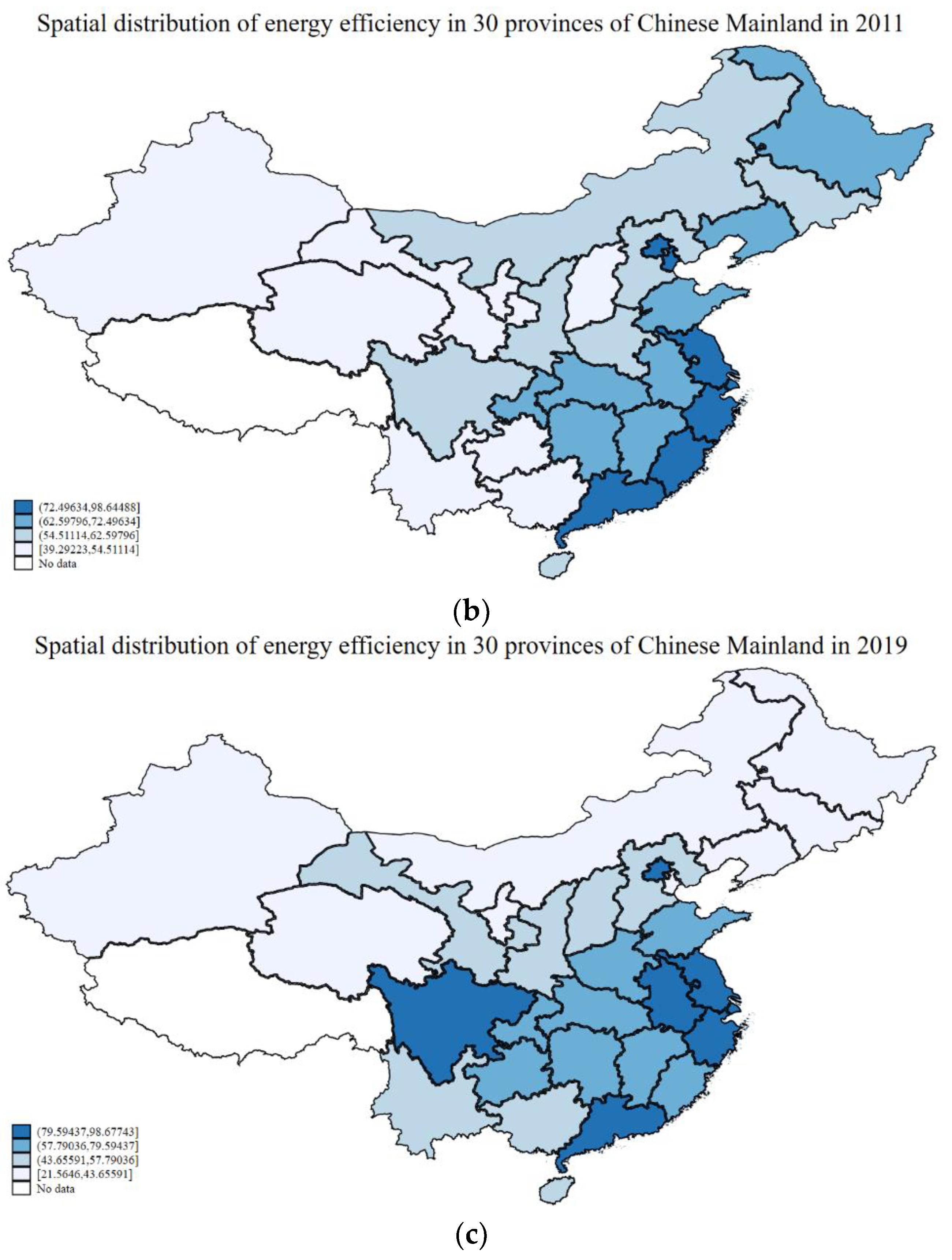
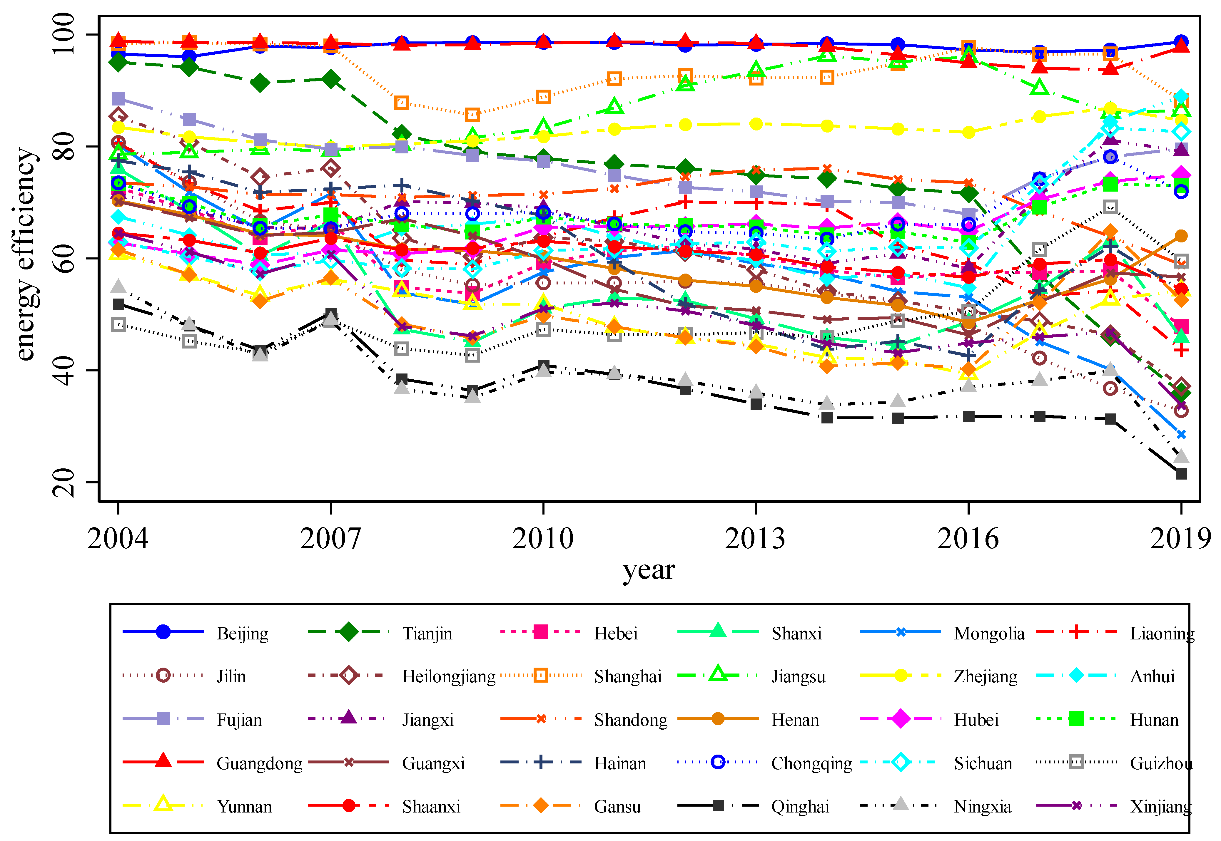
4.2. Estimation of Regional Energy Efficiency in China

The idea of the stochastic frontier model is similar to the data envelopment analysis (DEA). Both of the methods compare the current output with its possible maximum output. If the current output is closer to the maximum output, the efficiency will be higher; otherwise, the efficiency will be lower. An extreme case is that when the current output equals the maximum output, the efficiency value is 1 [29,30,32]. However, different from DEA, the stochastic frontier model assumes that the maximum possible output, namely, the production frontier, is not a deterministic frontier production function, but a non-deterministic stochastic frontier production function that may be affected by weather anomalies or production equipment errors; i.e.,
z i = f ( x i ; α ) + v i ,       i = 1 ,   ,   N
where x i represents the p-dimensional nonrandom vector of input of the given i-th producer; α is the corresponding p-dimensional parameter vector; and z i is the maximum possible output of the i-th producer under a given input x i , i.e., the production frontier. However, due to perturbations by random factors v i (such as weather conditions and equipment failures, and so on), the maximum output of the i-th producer is not the determined quantity f ( x i ; α ) but a random variable f ( x i ; α ) + v i . It is generally assumed that v i is independent and identically distributed in the normal distribution with mean 0 and variance σ v 2 , denoted as v i ~ N ( 0 , σ v 2 ) .
However, due to the influence of technical inefficiency and managers’ or employees’ inefficiency, the output of a producer cannot meet the production frontier, and therefore the stochastic frontier model can be expressed as
y i = f ( x i ; α ) + v i u i ,       i = 1 ,   ,   N
There are several variables different from Equation (1). Here, we assume that y i is the actual output of the i-th producer; u i follows half-normal distribution, i.e., u i = | U i | , U i ~ N ( 0 , σ u 2 ) ; and u i and v i are independent. Therefore, the efficiency of the i-th producer is measured by y i / [ f ( x i ; α ) + v i ] , so the efficiency is a real number valued at (0,1).
This paper adopts the stochastic frontier model improved by Battese and Coelli [30]. By taking labor (L), capital (K), and energy consumption (E) as input factors and real GDP as output [9], we construct a Cobb–Douglas stochastic frontier production model.
G D P i t = A L i t α 1 K i t α 2 E i t α 3 e v i t e u i ,       i = 1 ,   ,   N ; t = 1 ,   ,   T
After logarithmic treatment on both sides of the above equation, and denoting α 0 = l n A , we can obtain a linear form of the Cobb–Douglas stochastic frontier model.
l n G D P i t = α 0 + α 1 l n L i t + α 2 l n K i t + α 3 l n E i t + v i t u i ,       i = 1 ,   ,   N ; t = 1 ,   ,   T
where i denotes province and t denotes period. l n G D P i t is the logarithm of the actual GDP of the i-th province in the t-th period. In order to eliminate the influence of price factors, the real GDP here is obtained by dividing the nominal GDP by the GDP deflator, and the base period is 2004. L i t is the amount of labor put into production in period t of the i-th province. K i t is the capital stock in period t of the i-th province, which is calculated by the perpetual inventory method (PIM). Here, we adopt the depreciation rate estimated by Shan [52], and the annual fixed asset investment is adjusted by using the fixed asset investment price index based on 2004. E i t is the energy consumption of the i-th province in period t, and different types of energy are converted into standard coal. v i t is a random error, which is assumed to be independent and identically distributed to N ( 0 , σ v 2 ) . u i 0 is a non-negative random error capturing technical inefficiency, which is assumed to be independent and identically distributed to N + ( 0 , σ u 2 ) .
The energy efficiency of the i-th province is defined as
E E i = a c t u a l   o u t p u t s t o c h a s t i c   f r o n t i e r = G D P i t A L i t α 1 K i t α 2 E i t α 3 e v i t
Therefore, it is necessary to estimate conditional expectation E ( u i | v i t u i ) to get regional energy efficiency, as v it u i ^ = lnGDP it lnGDP it ^ ; therefore, the inefficiency term u i needs to be separated from the composite error term v i t u i (Greene [29] solved this problem theoretically). Further research by other scholars subsequently made the stochastic frontier model more practical [30,31].
Since the variation in regional energy efficiency is very small in the short term, we use the panel data time-invariant stochastic frontier model to estimate the energy efficiency of each year by rolling regression. The rolling window is 3 years (due to data limitation, the rolling window of the last year was set as 2 years). Specifically, the energy efficiency in 2004 was estimated using data from 2003 to 2005; the energy efficiency in 2017 was estimated using data from 2016 to 2018; the energy efficiency in 2018 was estimated using data from 2017 to 2019; and the energy efficiency in 2019 was estimated using data from 2018 to 2019.
According to the above method, the energy efficiency of the 30 provinces of Chinese Mainland from 2004 to 2019 was estimated, and its overview is shown in Figure 2.
As can be seen from Figure 2, the energy efficiency of most provinces fluctuates greatly. Some provinces’ energy efficiency decreases significantly, and some provinces’ energy efficiency increases significantly. However, Beijing, Guangdong, and Zhejiang, which have high energy efficiency, remain relatively stable. Next, we analyzed the basic situation of China’s energy efficiency from time and space perspectives.
The annual average energy efficiency of the 30 provinces in China from 2004 to 2019 is shown in Table 1. As can be seen from Table 1, China’s average energy efficiency fluctuates and declines from a low starting point. This is generally consistent with Lin and Xu [11] and Li et al. [9]. Due to China’s excessive pursuit of economic growth [14,53], the extensive economic growth mode driven by investment and energy leads to a gradual decline in energy efficiency.
Table 2 shows the provincial average energy efficiency of China from 2004 to 2019. It can be seen that there are great differences in energy efficiency among the provinces in China. The energy efficiency is relatively high in the eastern region, where Beijing, Shanghai, and Guangdong achieved an efficiency level of 90%, and Jiangsu and Zhejiang achieved an efficiency level of 80%. The energy efficiency of the central provinces is second, and that of the western underdeveloped provinces is the lowest; for example, the energy efficiency of Ningxia and Qinghai is lower than 40%. Our results are consistent with Yu [54] and Li et al. [9]. The higher energy efficiency in the eastern areas may be attributed to a higher level of economic development, better infrastructure, and citizens’ higher requirements for environmental protection. However, the situation in the economically backward central and western regions is the opposite.
As the provincial average energy efficiency does not show the spatial distribution and changes in energy efficiency, we depict the spatial distribution of China’s energy efficiency in representative years (2004, 2011, and 2019) in Figure 3.
As can be seen from Figure 3, China’s energy efficiency has obvious agglomeration characteristics; that is, the eastern region has high energy efficiency, followed by the central region, and the western region has the lowest energy efficiency. However, the energy efficiency in northeast China shows a downward trend over time. Next, we will conduct a more detailed empirical study.

5. Empirical Models

Environmental regulation and regional energy efficiency influence each other. On the one hand, environmental regulation imposes some constraints on the production technology, energy input, and energy structure adopted by enterprises, thus affecting energy efficiency in the region [7,11]. On the other hand, a change in regional energy efficiency is an important factor for the government to adjust environmental regulation policies, which has been ignored by most studies to date. Therefore, we need to establish a simultaneous equation model to investigate the interaction between environmental regulation and regional energy efficiency.
Meanwhile, due to local government competition, environmental regulation in this region is influenced by the environmental regulation of neighboring regions [15,16,17]. Moreover, due to technology spillover and resource flow, the local energy efficiency is also affected by the energy efficiency of neighboring regions; that is, energy efficiency has the feature of spatial agglomeration [8,9]. This is verified by the fact that the energy-efficient regions are clustered in the eastern region and the energy-inefficient regions are clustered in the central and western regions, as described in the previous section. Therefore, it is necessary to establish a spatial econometric model to investigate the spatial spillover effects of environmental regulation and regional energy efficiency.
We constructed the following simultaneous equation model with a spatial spillover effect. Using the estimation method given by Kelejian and Prucha [55], we analyzed the interactions between energy efficiency and environmental regulation and their spatial spillover effects under local government competition. At the same time, we consider the possible spatial correlation of the error terms.
E E i t = β 0 + β 1 j = 1 N w i j E E j t + β 2 j = 1 N w i j E R j t + β 3 E R i t + β X 1 + b 1 i + ε i t
ε i t = τ 1 j = 1 N w i j ε j t + ϵ i t
E R i t = γ 0 + γ 1 j = 1 N w i j E R j t + γ 2 j = 1 N w i j E E j t + γ 3 E E i t + γ X 2 + b 2 i + μ i t
μ i t = τ 2 j = 1 N w i j μ j t + ϑ i t
where i and j represent the provinces and t represents period. EE represents the energy efficiency and ER represents the intensity of environmental regulation. wij is the element in the i-th row and j-th column of the spatial weight matrix, indicating the spatial correlation between the i-th province and the j-th province. X 1 and X 2 are the vectors of control variables in Equations (6) and (8), respectively, and β and γ are the corresponding coefficient vectors. b 1 i and b 2 i denote individual effects, and ε i t and μ i t are random errors in Equations (6) and (8), respectively. Here we consider the possible spatial correlation of the error term in Equations (7) and (9), where ϵ i t and ϑ i t are independent and identically distributed random errors, respectively. It is assumed that the spatial weight matrices of Equations (6)–(9) are the same.
Simultaneous endogeneity and heteroscedasticity may exist in spatial simultaneous equation models, which makes the estimators inconsistent and inefficient. To deal with endogeneity, it is necessary to find suitable instrumental variables for the endogenous variables. Referring to the general method, the instrumental variables used here are all exogenous variables and their spatial lag terms [51]. For the heteroscedasticity problem, we use GLS to solve it. Firstly, the residual error is obtained by the estimation of the original Equations (6) and (8), and the coefficients τ 1 and τ 2 of the error term are estimated by GMM. Then, the Cochran–Orcutt transformation is performed on the original equation, and finally the spherical disturbance term is obtained [55].
In this paper, we use panel data in the analysis. However, the traditional generalized three-stage least squares (gs3sls) ignores the fixed effect of panel data, which may lead to biased or even inconsistent estimations. Therefore, we first perform fixed-effect transformation on the data, then specify the instrumental variables for the endogenous variables after transformation, and then perform generalized three-stage least squares regression [56].
The simultaneous equation model includes two endogenous variables, EE (regional energy efficiency) and ER (intensity of environmental regulation). EE was estimated in Section 3. For ER, the current measurement methods include three categories, such as the number of policies and regulations [51], pollutant discharge fee [51,57], and the investment in anti-pollution projects as percentage of GDP [11,40,58], etc. However, we believe that only the latter get the key point, because only pollution control actions are true environmental regulation. Therefore, we measure ER by the investment in anti-pollution projects as a percentage of GDP.
Based on previous work, the selected control variables X 1 that affect China’s regional energy efficiency include PGDP (regional GDP per capita), CSPW (capital stock per worker), and URB (urbanization rate), which reflect the regional economic conditions; OWS (ownership structure) and GOV (degree of government participation in economy), which reflect institutional factors; OFI (openness to foreign investment) and TRO (trade openness), which reflect openness; ENS (energy structure), which reflects the energy use structure; and IND (the ratio of industrial output to GDP) and SER (the ratio of service industry output to GDP), which reflect the industrial structure.
Among them, the level of regional economic development and local capital intensity affect the local energy production and utilization technology, the scale effect of energy consumption, energy consciousness, etc., subsequently affecting the energy efficiency. Therefore, we measured the regional economic development level with PGDP (regional GDP per capita) and measured the regional capital intensity level with CSPW (regional capital stock per worker), including both of them in the model as control variables [20,59]. URB (urbanization rate) is also a factor affecting energy efficiency. Due to the scale effect of urban heating and power supply, the energy efficiency of densely populated cities is often higher than that of rural areas. However, due to the fact that the per capita energy consumption in cities is much higher than that in rural areas, there is a great waste of energy, which may reduce the energy efficiency of cities [9,60,61].
In addition to the above economic factors, institutional factors may also affect regional energy efficiency. China’s ownership structure is different from that of most countries. China’s state-owned economy accounts for a large proportion of the national economy, and state-owned enterprises have a close relationship with the government. We can see state-owned enterprises get more preferential policies and exemption from pollution responsibility, which may affect regional energy efficiency. Here, we use “industrial sales of state-owned holding industrial enterprises divided by industrial sales of industrial enterprises above designated size” to represent the proportion of state-owned economy in the whole national economy to characterize OWS (ownership structure) [62]. Due to the serious waste of government consumption, the higher the GOV (degree of government participation in economy), the lower the energy efficiency [63]. GOV is measured by the proportion of fiscal expenditure in regional GDP.
As the energy density of different types of energy is different, ENS (energy structure) is an important factor affecting energy efficiency. Since China’s energy consumption is dominated by coal, the proportion of coal consumption in the total energy consumption is used to represent ENS [9,59].
Foreign investment may improve regional energy efficiency by bringing advanced production technology and management experience. Meanwhile, foreign investment from energy-intensive industries in developed countries may also reduce energy efficiency. The specific impact depends on which impact is dominant. Therefore, OFI (openness to foreign investment) needs to be controlled in the model; we measured it with the proportion of FDI to local GDP. As China has been at the low end of the global industrial chain for many years, and energy intensive products account for a large proportion of imports and exports, China’s trade openness may reduce the energy efficiency. Here, TRO (trade openness) is measured by the proportion of the total imports and exports in regional GDP [9].
Finally, because the energy intensity of the three industries is significantly different, the industrial structure affects the energy efficiency. Here, IND (the proportion of industrial added value in the GDP) and SER (the proportion of service industry added value in the GDP) are used to represent the industrial structure [9,64].
The selected control variables X 2 that affect the intensity of China’s environmental regulation include PGDP (regional GDP per capita) and URB (urbanization rate), which reflect the regional economic conditions; SFC (fiscal self-financing capacity), which reflects the financial situation of the region; OWS (ownership structure) and GOV (degree of government participation in economy), which reflect the institutional factors; OFI (openness to foreign investment), which reflects openness; ENS (energy structure), which reflects the energy-use structure; and GROW (regional economic growth rate) and UEM (unemployment rate), which reflect economic growth and unemployment.
Generally speaking, in areas with a high level of economic development and high urbanization rate, citizens have higher environmental requirements. Local governments may adjust the intensity of environmental regulation according to public expectations and realistic conditions. Therefore, it is necessary to control PGDP (regional GDP per capita) and URB (urbanization rate) in the equation of environmental regulation [16].
Meanwhile, the government needs to consider its own financial situation when carrying out environmental regulation. If the local financial resources are insufficient, strengthening the environmental regulation may hurt local investment, thus reducing the local tax revenue and worsening the local financial situation. Therefore, the regions with lower SFC (self-financing capacity) are more likely to reduce the intensity of environmental regulation [16]. We used “local fiscal revenue/local fiscal expenditure” to measure SFC.
In addition, environmental regulation in the areas with a higher proportion of state-owned economy may be reduced by the lobbying of state-owned enterprises. Therefore, OWS (ownership structure) may affect environmental regulation. However, in China, the regions with higher GOV (degree of government participation in economy) are mostly relatively poor, which are resource-based regions in the west. Due to the serious pollution in these areas, the intensity of environmental regulation has to be strengthened. Therefore, OWS and GOV need to be controlled [65,66].
It is well known that investment can directly promote economic growth. Since the Chinese government is keen to pursue economic growth, local governments may reduce the intensity of environmental regulation to attract foreign investment. Therefore, OFI (openness to foreign investment) may be a factor to be considered when the government carries out environmental regulation [53].
At the same time, differences in ENS (regional energy structure) lead to regional differences in environmental pollution, and then affect their environmental regulation policies. Therefore, governments tend to consider environmental regulation policies on the basis of their own energy structure.
Moreover, GROW (the economic growth rate) and UEM (unemployment rate) are important reference indicators for local governments to formulate policies [13,63,67], so it may be directly related to environmental regulation policies, but not directly related to regional energy efficiency. Here, GROW is calculated by the regional GDP index officially published by the National Bureau of Statistics of China, and UEM is measured by the registered urban unemployment rate published on this website.
Generally, a spatial econometric model is sensitive to the spatial weight matrix. Based on previous literature [8,9,15,16,68], we used five types of spatial weight matrices in the model to select the best model and test the robustness of the estimation results. (1) Contiguity weights: if two regions are adjacent, the weight of each other is 1, otherwise it is 0 (Guangdong and Hainan are regarded as adjacent regions). (2) Contiguity and economic distance weights: if two regions are adjacent, the PGDP (GDP per capita) of the neighboring region is used to measure the weight of the neighboring region on this region. (3) Geographical distance weights: the reciprocal of the geographical distance between the two regions is used as the weight of each other; i.e., w i j g = 1 / d i j , where d i j is the spherical distance between the provincial governments in the capital cities of province i and province j. We use the coordinate picker of the Baidu map to obtain the longitude and latitude coordinates of the provincial governments in provincial capitals and converted them into radian form. If the longitude and latitude of the two places were ( λ 1 , ϕ 1 ) and ( λ 2 , ϕ 2 ) , respectively, the spherical distance between the two places can be obtained by the equation d = 2 r a r c s i n ( s i n 2 ( ϕ 2 ϕ 1 2 ) + cos ( ϕ 2 ) cos ( ϕ 1 ) s i n 2 ( λ 2 λ 1 2 ) ) , where r = 6372 (kilometers) is the radius of the earth. (4) Economic distance weights: the reciprocal of the difference between the two regions’ PGDP (GDP per capita) is used to measure the weight of the two provinces; i.e., w i j e = 1 / | G D P i G D P j | , where the two provinces with a smaller economic gap have a greater weight because they often compete and cooperate with each other. (5) Geographical distance and economic distance weights: the weight is w i j = w i j g w i j e , which is a combination of the geographical distance weight and economic distance weight. All spatial weight matrices were normalized.
In order to intuitively observe the summary information of each variable, we show the descriptive statistics of each variable in Table 3.

6. Empirical Results and Discussion

The empirical research follows the framework shown in Figure 4. Firstly, the causality analysis of environmental regulation and energy efficiency was carried out. If it is confirmed that environmental regulation and energy efficiency are mutually causal, the simultaneous equation model can be used. Next, the spatial correlation test of environmental regulation and energy efficiency was carried out. If it was confirmed that they are spatially correlated, the spatial simultaneous equation model was used. Then, the model was estimated under the five spatial weight matrices, and the estimation results were analyzed. Finally, we tested the robustness of the estimation results.

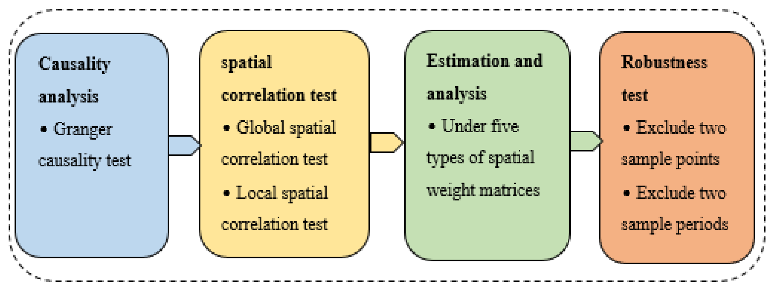
6.1. Causality Analysis

Before estimating, we needed to make a causality analysis of the environmental regulation (ER) and energy efficiency (EE). Here, the Granger causality test of panel data was adopted to verify the causality between ER and EE. The lag order was selected according to the BIC criterion. The results are shown in Table 4.
It is easy to see from Table 4 that “EE does not Granger-cause ER” and “ER does not Granger-cause EE” are rejected at the significance level of 1%; that is, environmental regulation and energy efficiency are mutually causal. Therefore, it is reasonable to use a simultaneous equation model to study their interaction.

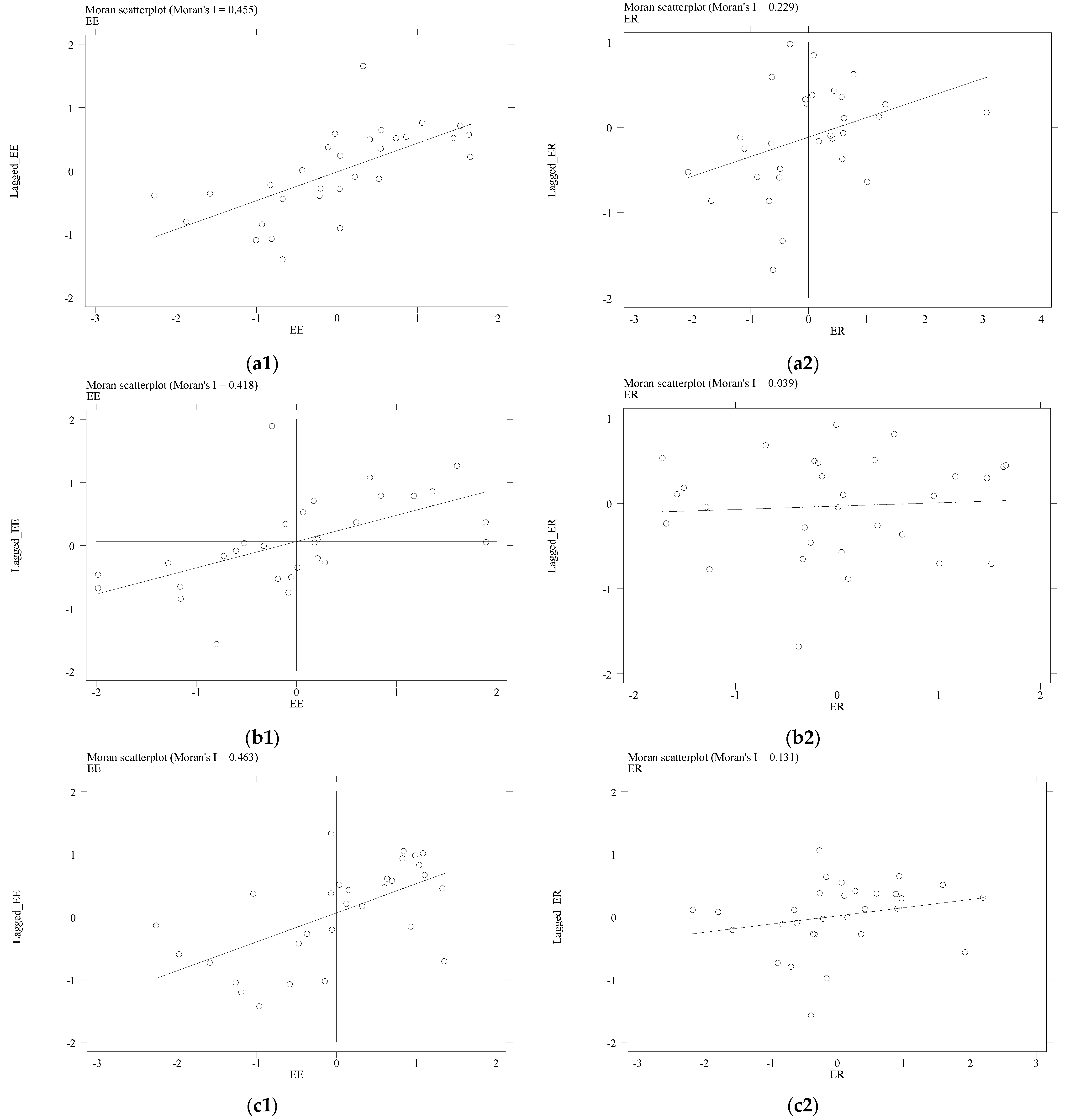
6.2. Global Spatial Correlation Test

We use Moran’s I to test the global spatial correlation of regional energy efficiency and environmental regulation intensity under different spatial weight matrices. Since the test results are similar, we only report the results under the simple contiguity weight matrix.
Table 5 reports the global correlation test results of regional energy efficiency and environmental regulation intensity. It can be found that the null hypothesis—that there is no spatial correlation of regional energy efficiency—is rejected at a significance level of 1% for all years, which indicates that China’s regional energy efficiency has strong spatial correlation. However, the spatial correlation of environmental regulation is not significant in 9 of the 16 years, while it is relatively significant in the other 7 years. This shows that the environmental regulatory competition of local governments in China is sometimes strong and sometimes weak.

6.3. Local Spatial Correlation Test

The global Moran’s I only tests the global spatial correlation, but not the local spatial correlation. Therefore, we report the local Moran scatter plots (MSP) of regional energy efficiency and environmental regulation in Figure 5 to further explore the local spatial correlation of the two. Considering that there are many years from 2004 to 2019, and the spatial correlation characteristics of regional energy efficiency and environmental regulation intensity are similar in most years, only the representative Moran scatter plots of 2004, 2011, and 2019 are shown here.
As can be seen from Figure 5, most observed values of the local Moran’s I of regional energy efficiency fall into the first quadrant and the third quadrant in all years. Statistically speaking, the types of spatial correlation are mainly high–high and low–low; that is, provinces with high energy efficiency are more likely to be surrounded by provinces with high energy efficiency, and provinces with low energy efficiency are more likely to be surrounded by provinces with low energy efficiency. This is consistent with the results of Li et al. [9] and Yu [54]. However, most observed values of Moran’s I of local environmental regulation intensity fall into the first quadrant and the third quadrant in 2004 and 2019, and the distribution of Moran’s I in 2011 is relatively irregular, which indicates that local governments do not continuously compete in environmental regulation, which is consistent with the conclusion of the global spatial correlation test.
The above results show that it is necessary to consider spatial correlation in the empirical study. If we omit the spatial correlation in the empirical model, the estimation results may be biased or even inconsistent.

6.4. Estimation Results and Analysis

According to the order condition and rank condition of the simultaneous equation models, Equations (6)–(9), Equations (6) and (8) are over identified, so the model can be estimated. In order to make the model easier to explain, we log-transformed the endogenous variables and some economic variables, including EE, ER, PGDP, and CSPW. The system estimation results of the coefficients are shown in Table 6 and Table 7.
Table 6 and Table 7 report the system estimation results of the simultaneous equation models under five types of spatial weight matrices, where W_EE and W_ER are the spatial lag terms of EE (regional energy efficiency) and ER (environmental regulation intensity), respectively. It can be seen from Table 6 and Table 7 that the signs of most of the estimated coefficients of explanatory variables are the same under the five types of spatial weight matrices, indicating that our model is quite robust. According to the adjusted R-square of the simultaneous equation model reported in Table 8, the goodness of fit under the five types of spatial weight matrices is relatively similar. Nevertheless, it is relatively better to use the spatial weight matrix of geographical distance and economic distance for estimation. Therefore, we mainly use the estimation results under this spatial weight matrix as the benchmark when analyzing the estimation results.
From the estimated results of the regression equation of regional energy efficiency in Table 6, we find that the coefficients of W_EE and ER are significantly positive, while the coefficient of W_ER is small and only weakly significant. Under the spatial weight matrix of geographical distance and economic distance, the coefficient of environmental regulation on energy efficiency in this region is 1.0404, which is significantly positive; that is, on average, if the energy efficiency of the surrounding regions is increased by 1%, the energy efficiency of the region will be increased by 1.0404%, otherwise the local energy efficiency may be reduced by 1.0404%. This shows that the energy efficiency has strong spatial accumulation characteristics, and the surrounding regions can affect the energy efficiency of the region through resource flow, technology spillover, and other ways. This is consistent with the empirical results of Li et al. [9] and Du et al. [69]. Meanwhile, environmental regulation has a significantly positive effect on energy efficiency; that is, under the current situation in China, strengthening environmental regulation can improve energy efficiency. In other words, China’s environmental regulation policies are effective. On average, if the intensity of environmental regulation is increased by 1%, the energy efficiency of this region can be increased by 0.2777%, which indicates that environmental regulation can promote Chinese enterprises to save energy or improve energy utilization efficiency. On the contrary, if the regional environmental regulation intensity is reduced, the regional energy efficiency will deteriorate [38,39,40,46,70,71]. However, the coefficient sign of W_ER is inconsistent and weakly significant, which means that the environmental regulation in the surrounding regions has no significant direct impact on the energy efficiency of this region.
From the estimated results of the regression equation of environmental regulation in Table 7, we learned that the coefficients of W_ER and EE are significantly positive, while the coefficient of W_EE is significantly negative under most spatial weight matrices. Specifically, on average, if the environmental regulation intensity of the surrounding provinces is increased by 1%, the province’s environmental regulation intensity will be increased by 0.6075%. On the contrary, if the surrounding provinces reduce the environmental regulation intensity by 1%, the province will generally follow up to reduce the environmental regulation intensity by 0.6075%. This shows that under the “Promotion Tournament” mode in China, there is inter-regional competition among local governments on the whole [14]. This competition of environmental regulation is mainly in the form of mutual imitation; in other words, environmental regulation intensity tends to rise and fall at the same time. The coefficient of energy efficiency to environmental regulation in this region is 1.5981, which is significantly positive. This means that if the local energy efficiency is increased by 1%, the intensity of local environmental regulation will be increased by 1.5981%. On the contrary, if the local energy efficiency is reduced by 1%, the local environmental regulation intensity will be reduced by 1.5981%. This may be due to the fact that most local governments pay more and more attention to energy efficiency when they pursue energy efficiency, while energy efficiency is more and more ignored when they do not pursue energy efficiency. It can be seen from Table 1 that China’s regional energy efficiency is decreasing year by year. Therefore, local governments in China tend to “race to the bottom” in environmental regulation. The coefficient of W_EE under most spatial weight matrices is significantly negative. It means that when the energy efficiency of the surrounding provinces is improved, the province may significantly reduce the intensity of environmental regulation. This may be because the local government expects that the improvement in energy efficiency in surrounding provinces will have a positive impact on local energy efficiency. For the sake of free riding, the local government significantly reduces the intensity of environmental regulation.
Combining the coefficients of the two endogenous variables and their spatial lag terms, we can sketch the story of local government competition, environmental regulation, and regional energy efficiency in China. Due to China’s top–down political system, the promotions of lower-level officials are mainly determined by higher-level officials according to certain criteria (similar to KPI). For the sake of fairness, due to the Chinese people’s desire for wealth and other aspects, the evaluation standard of Chinese government officials is mainly the economic growth rate (although in recent years China has claimed to take environmental improvement as one of the evaluation objectives, the economic growth rate still occupies the main weight in the evaluation index) [14]. Since it is investment that can significantly stimulate economic growth in the short term, most of the local government officials in China mainly focus on attracting investment, and even lower energy and environmental standards in exchange for enterprise investment when necessary. Therefore, in order to attract investment, most provinces tend to reduce the intensity of environmental regulation [51]. For a province, if the environmental regulation intensity of the surrounding provinces decreases tentatively, due to local government competition, the province will also reduce the intensity of environmental regulation in order to retain investment, which will lead to a decline in energy efficiency in the province. However, due to the spatial spillover effect of energy efficiency, the decrease in energy efficiency may lead to a decrease in energy efficiency in the surrounding areas [69]. Because the coefficient of energy efficiency to environmental regulation is positive, the reduction in energy efficiency in surrounding areas will make the surrounding areas pay less attention to energy efficiency, and may continue to reduce the energy efficiency target and the intensity of environmental regulation. In this way, the vicious circle continues. Although the average intensity of environmental regulation has increased for several years due to the serious environmental degradation in China, generally speaking, China’s energy efficiency and environmental regulation intensity have been declining.
For the common control variables in the two equations, the sign of their coefficients is mostly consistent with our expectation. PGDP (Regional GDP per capita) and URB (urbanization) can significantly promote EE (regional energy efficiency), because the areas with high PGDP and URB generally have high energy utilization technology and the advantage of a scale economy [8]. However, PGDP cannot promote the strengthening of ER (environmental regulation). This may be due to the high energy efficiency and environmental quality in developed areas, where a low-level environmental regulation can meet the environmental needs. The coefficient of URB on ER is not significant. This may be because the environmental protection demands of urban residents have not put pressure on local governments [8]. The coefficient of OWS (ownership structure, measured by the proportion of the state-owned economy in the national economy) on EE is not significant. This shows that although China’s state-owned enterprises enjoy preferential policies, they do not have a negative impact on energy efficiency due to economies of scale (China’s state-owned enterprises are usually large-scale). This is different from the research results of Zhao and Lin [62] on China’s textile industry. The coefficient of OWS on ER is negative, but it is significant under one spatial weight matrix. To some extent, this indicates that state-owned enterprises may lobby local governments to relax environmental regulation. However, GOV (degree of local government participation in the economy) significantly inhibits the regional energy efficiency. This is because the Chinese government’s consumption is unconstrained and unsupervised, which consumes a lot of energy but creates little value, resulting in a low energy efficiency. On the contrary, GOV promotes environmental regulation. This is because most of the regions with big GOVs are underdeveloped resource-based provinces in the west, and environmental regulation must be strengthened to control heavy pollution caused by resource exploitation. OFI (degree of openness to foreign investment) promotes the improvement of regional energy efficiency, but the coefficient is small, indicating that the effect is limited. Meanwhile, the coefficient of OFI to ER is not significant. This may be due to the fact that foreign investment is stably concentrated in the developed eastern coastal provinces, and the overall impact on environmental regulation is relatively weak [53]. Finally, ENS (energy structure) suppresses regional energy efficiency, because coal is a common energy with a very low energy density. The higher its consumption proportion, the lower the energy efficiency [9,59]. The coefficient of ENS to ER is significant under two spatial weight matrices. Therefore, it can be considered that the influence of ENS on environmental regulation is limited.
For the other control variables in the regression equation of regional energy efficiency, CSPW (capital stock per worker) and IND (industry) significantly inhibited the improvement of energy efficiency, because the extensive growth of China’s economy increased the quantity, but it paid a large energy cost [9,53,59]. However, the impact of SER (service industry) on EE is not significant, which indicates that the energy efficiency of China’s service industry is not yet high. The impact of TRO (trade openness) on EE is also significantly negative. This is because the bulk of China’s foreign trade is in highly polluting, energy-hungry industries, which further confirms the energy cost of China’s extensive growth [72].
For the other control variables in the regression equation of environmental regulation, SFC (self-financing capacity) has a positive impact on ER, but it is significant only under the spatial weight matrix of economic distance. This shows that local governments only sometimes weigh the environmental regulation according to their own financial resources [16,53]. Similarly, GROW (regional economic growth rate) is significantly positively correlated with ER. When the economic growth slows down, local governments will relax environmental regulation, and when the economic growth speeds up, they will strengthen environmental regulation. However, the impact of UEM (unemployment) on ER is not significant. On the one hand, it may be due to the sampling bias of the unemployment rate in China’s urban survey, which cannot reflect China’s real unemployment rate. On the other hand, it may be due to China’s top–down political system, and government officials paying insufficient attention to the welfare of the people.
From the regression results, it can be seen that the energy efficiency of the surrounding areas, the local economic development level and local environmental regulation are the most important factors affecting energy efficiency. Therefore, it is effective to promote environmental sustainability from these aspects.

6.5. Robustness Test

In Section 6.4, we used five different spatial weight matrices and got similar estimation results. This verifies the robustness of our conclusions to some extent. However, further robustness tests were necessary. The further robustness tests we designed mainly included the following two aspects: (1) sensitivity analysis by excluding the data of some years; and (2) sensitivity analysis by excluding the data of some sample points. Of interest are the coefficients of the endogenous variables (environmental regulation and regional energy efficiency) and the coefficients of their spatial lag terms. Meanwhile, we found that the sign and magnitude of the coefficient estimates of the control variables in the robustness test are similar to the full sample estimation results. To save space and highlight key points, we do not report the estimation results of the control variables, but only the estimation results of the endogenous variables and their spatial lag terms.
We first excluded the data of 2018 and 2019, and retained the panel data of 30 provinces in Chinese mainland from 2004 to 2017 for estimation. The system estimation results of the endogenous variables are shown in Table 9. Then, we excluded the data of Chongqing (a relatively rich region) and Hainan Province (a relatively poor region), and retained the panel data of the other 28 provinces from 2004 to 2019 for estimation. The system estimation results of the endogenous variables are shown in Table 10.
The results in Table 9 and Table 10 are obvious. After excluding some sample data, the symbols of the coefficients of endogenous variables and their spatial lag terms estimated by using five spatial weight matrices are almost consistent with the results estimated by using full samples. There is only a certain difference in the size of the coefficients. To some extent, this shows that our conclusions are quite robust in both the time and regional dimensions.

6.6. Discussion

Energy efficiency is the key to ensure the coordinated development of the economy and environment, so it has been highly regarded by governments and scholars all over the world. Most countries adopt environmental regulation measures to influence energy efficiency. Scholars also adopt various methods to study the impact of environmental regulation on energy efficiency. Most of these methods are single equation models. However, changes in energy efficiency can also affect environmental regulation. Therefore, the correlation between environmental regulation and energy efficiency leads to the endogeneity problem in a single equation model. Although the instrumental variable method can solve the endogeneity problem in theory, it is usually difficult to find a satisfactory instrumental variable in practical research. Besides, due to interregional economic cooperation and resource flows in reality, local energy efficiency tends to correlate with that of the surrounding areas. Moreover, due to the competition and cooperation of local governments, local environmental regulation is also related to the environmental regulation of surrounding areas. Therefore, it is necessary to study the interaction between the local environmental regulation and surrounding environmental regulation, the interaction between the local energy efficiency and surrounding energy efficiency, and the interaction between the environmental regulation and energy efficiency under a unified framework. By using the spatial simultaneous equation model, this paper studied the spatial effects between environmental regulation and energy efficiency and their interactions under a unified framework, and solved the above problems better. These problems cannot be solved well by using single equation econometric models or non-spatial econometric models. The empirical results obtained in this study are satisfactory.
The empirical results of this study show that China’s environmental regulation has a positive effect on energy efficiency. At the same time, energy efficiency also has a positive effect on environmental regulation. Therefore, strengthening environmental regulation can effectively improve China’s overall energy efficiency and promote their benign interaction. The empirical results also show that both environmental regulation and energy efficiency have positive spatial effects. Therefore, China should create a good interregional incentive mechanism, promote the positive impact between environmental regulation and energy efficiency, and avoid the negative effect between environmental regulation and energy efficiency. In addition, the energy efficiency of the surrounding areas, the level of local economic development, and the local environmental regulation are the most important factors affecting energy efficiency. Therefore, strengthening regional economic and technical cooperation, focusing on the development of local economy and reasonable environmental regulation, are powerful measures to improve local energy efficiency.
This study discussed the spatial effects of environmental regulation and energy efficiency and their interactions in China. This provides important empirical evidence for more reasonable environmental regulation in China, which would lead to sustainable development of China’s economy and environment. In addition, this study enriches the research on environmental regulation and energy efficiency.

7. Conclusions and Policy Recommendations

7.1. Conclusions

This paper discussed the decision mechanism of local government environmental regulation, the interaction between environmental regulation and regional energy efficiency, and the spatial spillover effects of both under local government competition. The main conclusions are as follows. (1) There is a significant positive correlation between environmental regulation and regional energy efficiency. Strengthening the intensity of environmental regulation may lead to higher energy efficiency. At the same time, the improvement in energy efficiency may also stimulate local governments to strengthen the intensity of environmental regulation. (2) Regional energy efficiency has a significant positive spatial spillover effect; that is, the improvement in energy efficiency in the surrounding areas is conducive to the improvement of the local energy efficiency, and vice versa. (3) Environmental regulation has a significant positive spatial spillover effect. In the context of local government competition, China’s inter-provincial environmental regulation is manifested in the form of “imitation competition”; specifically, if the surrounding provinces reduce their environmental regulation intensity, this province will follow up.

7.2. Managerial Implication

Based on the above conclusions and the estimation results, we can get the following policy inspirations. (1) As a result of interregional exchanges and integration, the improvement in energy efficiency in the surrounding areas benefits the local energy efficiency. Therefore, it is necessary to strengthen the interregional industrial development links and promote a coordinated development of interregional industries. (2) China’s inter provincial environmental regulation is embodied in the form of “imitation competition”, which may lead to the fact that the local environmental regulation policy is not optimal. Therefore, local governments should reasonably formulate environmental regulation policies according to local economic development and environmental conditions. At present, China should establish some higher level multi-provincial environmental management departments that operate independently of local governments. This would prevent local governments from competing to reduce the intensity of environmental regulation. (3) Due to the positive interaction between environmental regulation and energy efficiency, improving energy efficiency and strengthening environmental regulation will help to promote the benign interaction between energy efficiency and environmental regulation in China. Therefore, local governments should give policy support to enterprises to improve energy technology. At the same time, the central government should reduce the political cost of local governments to implement environmental regulation. (4) The increase of urbanization rate is conducive to the improvement of energy technology and energy intensive utilization. Therefore, China should reduce the barriers to urbanization and continue to improve the urbanization rate. (5) Since coal and other fossil fuels are detrimental to China’s energy efficiency, China needs to continue to reduce the share of fossil fuels in total energy consumption, and increase the share of new energy sources, such as photovoltaic, wind power, and hydropower. (6) The level of economic development and openness to foreign investment can promote the improvement of China’s energy efficiency. Therefore, China should continue to adhere to reform and opening up, develop its economy, and learn advanced technology and management experience from developed countries. However, China needs to change the previous extensive investment-driven growth model and embrace sustainable development.

7.3. Limitations and Prospects

This study also has some limitations. First, due to data availability, some variables that may affect energy efficiency and environmental regulation cannot be included in the empirical study, such as the vintage of the power generation. However, we have done our best to collect data and include possible influencing factors into the model. Second, our sample period is 2004–2019. However, the intensified trade friction between China and the United States in 2018 may have affected the behavior of Chinese economic actors and disrupted economic laws. Therefore, it is necessary to exclude the data of some special years for research. We excluded the data of 2018–2019 for the robustness test, and the findings were similar to the estimates for the full sample period. This shows that our findings are still valid. Finally, the mechanism of the relationship between environmental regulation and energy efficiency is revealed through natural language. Compared with establishing mathematical models and then strictly carrying out logical reasoning, this is not rigorous enough. However, we have collected a large number of references to explain their logical relationship.
Future research on environmental regulation and energy efficiency can be carried out from the following aspects: (1) With the advent of the era of big data, we can collect data through various technologies and approaches. Issues related to energy efficiency can be better studied using big data. (2) Mathematical models can be established. Mathematical models perform rigorous logical reasoning under the given assumptions. This avoids the uncertainty of verbal derivation. (3) The estimation model of energy efficiency can be improved to make a more reasonable estimation of energy efficiency. (4) The effect of different types of environmental regulations on energy efficiency is valuable. The energy efficiency-related issues of different sub-sectors and different sub-regions are also worthy of further study.

Author Contributions

Conceptualization, F.J. and M.K.; methodology, F.J. and M.K.; software, F.J.; validation, M.K.; formal analysis, F.J. and M.K.; investigation, F.J. and M.K.; resources, F.J. and M.K.; data curation, F.J.; writing—original draft preparation, M.K.; writing—review and editing, F.J.; visualization, F.J. and M.K.; supervision, F.J. and M.K.; project administration, F.J. and M.K.; funding acquisition, F.J. All authors have read and agreed to the published version of the manuscript.

Funding

This research was funded by MOE Project of Humanities and Social Sciences in China, grant number 19YJC790051, Education Research Project of Young and Middle-aged Teachers of Fujian Province in China, grant number JAT170119, Major Project of Social Science Research Base of Fujian Province in China, grant number FJ2019JDZ015.

Institutional Review Board Statement

Not applicable.

Informed Consent Statement

Not applicable.

Data Availability Statement

Please contact the authors via email for the data.

Conflicts of Interest

The authors declare no conflict of interest.

References

  1. Rehman, A.; Ma, H.; Ozturk, I.; Murshed, M.; Dagar, V. The dynamic impacts of CO2 emissions from different sources on Pakistan’s economic progress: A roadmap to sustainable development. Environ. Dev. Sustain. 2021, 23, 17857–17880. [Google Scholar] [CrossRef]
  2. Davis, S.J.; Caldeira, K.; Matthews, H.D. Future CO2 Emissions and Climate Change from Existing Energy Infrastructure. Science 2010, 329, 1330–1333. [Google Scholar] [CrossRef] [Green Version]
  3. Alvarado, R.; Ortiz, C.; Jiménez, N.; Ochoa-Jiménez, D.; Tillaguango, B. Ecological footprint, air quality and research and development: The role of agriculture and international trade. J. Clean. Prod. 2021, 288, 125589. [Google Scholar] [CrossRef]
  4. Ortiz, C.; Sarrias, M. Estimating the non-pecuniary benefit of engaging in pro-environmental behaviors: Incorporating both heterogeneous preferences and income endogeneity. J. Environ. Manag. 2022, 302, 114040. [Google Scholar] [CrossRef]
  5. Irfan, M.; Elavarasan, R.M.; Ahmad, M.; Mohsin, M.; Dagar, V.; Hao, Y. Prioritizing and overcoming biomass energy barriers: Application of AHP and G-TOPSIS approaches. Technol. Forecast. Soc. Chang. 2022, 177, 121524. [Google Scholar] [CrossRef]
  6. Li, H.; Zhang, J.; Wang, C.; Wang, Y.; Coffey, V. An evaluation of the impact of environmental regulation on the efficiency of technology innovation using the combined DEA model: A case study of Xi’an, China. Sustain. Cities Soc. 2018, 42, 355–369. [Google Scholar] [CrossRef]
  7. Wu, J.; Yang, J.; Zhou, Z. How does environmental regulation affect environmental performance? A case study of China’s regional energy efficiency. Expert Syst. 2020, 37, e12326. [Google Scholar] [CrossRef]
  8. Zhu, Y.; Wang, Z.; Qiu, S.; Zhu, L. Effects of environmental regulations on technological innovation efficiency in China’s industrial enterprises: A spatial analysis. Sustainability 2019, 11, 2186. [Google Scholar] [CrossRef] [Green Version]
  9. Li, K.; Fang, L.; He, L. How urbanization affects China’s energy efficiency: A spatial econometric analysis. J. Clean. Prod. 2018, 200, 1130–1141. [Google Scholar] [CrossRef]
  10. Zhao, H.; Guo, S.; Zhao, H. Provincial energy efficiency of China quantified by three-stage data envelopment analysis. Energy 2019, 166, 96–107. [Google Scholar] [CrossRef]
  11. Lin, J.; Xu, C. The impact of environmental regulation on total factor energy efficiency: A cross-region analysis in China. Energies 2017, 10, 1578. [Google Scholar] [CrossRef] [Green Version]
  12. Ma, D.; Xiong, H.; Zhang, F.; Gao, L.; Zhao, N.; Yang, G.; Yang, Q. China’s industrial green total-factor energy efficiency and its influencing factors: A spatial econometric analysis. Environ. Sci. Pollut. Res. 2022, 29, 18559–18577. [Google Scholar] [CrossRef] [PubMed]
  13. Cao, Y.; Wan, N.; Zhang, H.; Zhang, X.; Zhou, Q. Linking environmental regulation and economic growth through technological innovation and resource consumption: Analysis of spatial interaction patterns of urban agglomerations. Ecol. Indic. 2020, 112, 106062. [Google Scholar] [CrossRef]
  14. Zhou, L. Governing China’s local officials: An analysis of promotion tournament model. Econ. Res. J. 2007, 7, 36–50. [Google Scholar]
  15. Fredriksson, P.G.; Millimet, D.L. Strategic Interaction and the Determination of Environmental Policy across U.S. States. J. Urban Econ. 2002, 51, 101–122. [Google Scholar] [CrossRef]
  16. Konisky, D.M. Regulatory competition and environmental enforcement: Is there a race to the bottom? Am. J. Polit. Sci. 2007, 51, 853–872. [Google Scholar] [CrossRef]
  17. Woods, N.D. Interstate competition and environmental regulation: A test of the race-to-the-bottom thesis. Soc. Sci. Q. 2006, 87, 174–189. [Google Scholar] [CrossRef]
  18. Ching-Cheng, L.; Liang-Chun, L. Evaluating the energy efficiency of European Union countries: The dynamic data envelopment analysis. Energy Environ. 2019, 30, 27–43. [Google Scholar]
  19. Rakshit, I.; Mandal, S.K. A global level analysis of environmental energy efficiency: An application of data envelopment analysis. Energy Effic. 2020, 13, 889–909. [Google Scholar] [CrossRef]
  20. Liu, W.; Lin, B. Analysis of energy efficiency and its influencing factors in China’s transport sector. J. Clean. Prod. 2018, 170, 674–682. [Google Scholar] [CrossRef]
  21. Masuda, K. Energy efficiency of intensive rice production in Japan: An application of data envelopment analysis. Sustainability 2018, 10, 120. [Google Scholar] [CrossRef] [Green Version]
  22. Hafiz Muhammad Abrar, I.; Majeed, S.; Alison, B.; Sara, R.; Azeem, K. Energy efficiency outlook of New Zealand dairy farming systems: An application of data envelopment analysis (DEA) approach. Energies 2020, 13, 251. [Google Scholar]
  23. Babazadeh, R.; Razmi, J.; Rabbani, M.; Pishvaee, M.S. An integrated data envelopment analysis–mathematical programming approach to strategic biodiesel supply chain network design problem. J. Clean. Prod. 2017, 147, 694–707. [Google Scholar] [CrossRef]
  24. Cook, W.D.; Tone, K.; Zhu, J. Data envelopment analysis: Prior to choosing a model. Omega 2014, 44, 1–4. [Google Scholar] [CrossRef]
  25. Yang, H.; Shi, D. Energy-Efficiency methods and comparing the energy efficiencies of different areas in China. Econ. Theory Bus. Manag. 2008, 3, 12–20. [Google Scholar]
  26. Aigner, D.; Lovell, C.A.K.; Schmidt, P. Formulation and estimation of stochastic frontier production function models. J. Econom. 1977, 6, 21–37. [Google Scholar] [CrossRef]
  27. Battese, G.E.; Corra, G.S. Estimation of a production frontier model: With application to the pastoral zone of eastern Australia. Aust. J. Agric. Econ. 1977, 21, 169–179. [Google Scholar] [CrossRef] [Green Version]
  28. Meeusen, W.; van den Broeck, J. Technical efficiency and dimension of the firm: Some results on the use of frontier production functions. Empir. Econ. 1977, 2, 109–122. [Google Scholar] [CrossRef]
  29. Greene, W.H. Maximum likelihood estimation of econometric frontier functions. J. Econom. 1980, 13, 27–56. [Google Scholar] [CrossRef]
  30. Battese, G.E.; Coelli, T.J. A model for technical inefficiency effects in a stochastic frontier production function for panel data. Empir. Econ. 1995, 20, 325–332. [Google Scholar] [CrossRef] [Green Version]
  31. Wang, H.-J.; Ho, C.-W. Estimating fixed-effect panel stochastic frontier models by model transformation. J. Econom. 2010, 157, 286–296. [Google Scholar] [CrossRef] [Green Version]
  32. Al-Gasaymeh, A. Bank efficiency determinant: Evidence from the gulf cooperation council countries. Res. Int. Bus. Financ. 2016, 38, 214–223. [Google Scholar] [CrossRef]
  33. Ferreira, M.D.P.; Féres, J.G. Farm size and Land use efficiency in the Brazilian Amazon. Land Use Policy 2020, 99, 104901. [Google Scholar] [CrossRef]
  34. Miao, C.; Meng, X.; Duan, M.; Wu, X. Energy consumption, environmental pollution, and technological innovation efficiency: Taking industrial enterprises in China as empirical analysis object. Environ. Sci. Pollut. Res. 2020, 27, 34147–34157. [Google Scholar] [CrossRef]
  35. Mandal, S.K. Do undesirable output and environmental regulation matter in energy efficiency analysis? Evidence from Indian Cement Industry. Energy Policy 2010, 38, 6076–6083. [Google Scholar] [CrossRef]
  36. Bi, G.-B.; Son, W.; Zhou, P.; Liang, L. Does environmental regulation affect energy efficiency in China’s thermal power generation? Empirical evidence from a slacks-based DEA model. Energy Policy 2014, 66, 537–546. [Google Scholar] [CrossRef]
  37. Kneller, R.; Manderson, E. Environmental regulations and innovation activity in UK manufacturing industries. Resour. Energy Econ. 2012, 34, 211–235. [Google Scholar] [CrossRef]
  38. Wang, X.; Du, L. Analysis of China’s total-factor energy efficiency and its convergence under environmental regulation. J. Inf. Comput. Sci. 2015, 12, 4281–4289. [Google Scholar] [CrossRef]
  39. Zhang, C.; He, W.D.; Hao, R. Analysis of environmental regulation and total factor energy efficiency. Curr. Sci. 2016, 110, 1958–1968. [Google Scholar] [CrossRef]
  40. Pan, X.; Ai, B.; Li, C.; Pan, X.; Yan, Y. Dynamic relationship among environmental regulation, technological innovation and energy efficiency based on large scale provincial panel data in China. Technol. Forecast. Soc. Chang. 2019, 144, 428–435. [Google Scholar] [CrossRef]
  41. Barbera, A.J.; McConnell, V.D. The impact of environmental regulations on industry productivity: Direct and indirect effects. J. Environ. Econ. Manag. 1990, 18, 50–65. [Google Scholar] [CrossRef]
  42. Jorgenson, D.W.; Wilcoxen, P.J. Environmental regulation and US economic growth. RAND J. Econ. 1990, 21, 314–340. [Google Scholar] [CrossRef]
  43. Lanoie, P.; Patry, M.; Lajeunesse, R. Environmental regulation and productivity: Testing the porter hypothesis. J. Product. Anal. 2008, 30, 121–128. [Google Scholar] [CrossRef]
  44. Yang, H.; Wang, X. Is Environmental Regulation an Effective Way to Prevent Energy Rebound Effect? J. Manag. 2021, 34, 74–91. [Google Scholar]
  45. Yu, B.; Jin, G.; Cheng, Z. Economic effects of environmental regulations: “emission reduction” or “efficiency enhancement”. Stat. Res. 2019, 36, 88–100. [Google Scholar]
  46. Peng, S. China’s total factor energy efficiency evaluation: Based on three stage global undesirable-hybrid-slack-based-model. Econ. Probl. 2020, 1, 11–19. [Google Scholar]
  47. Gao, Z.; You, J. The intensity of environmental regulation and the total factor energy efficiency of China. Comp. Econ. Soc. Syst. 2015, 111–123. Available online: https://kns.cnki.net/kcms/detail/detail.aspx?FileName=JJSH201506012&DbName=CJFQ2015 (accessed on 1 June 2022).
  48. Li, Y.; Xu, X.; Zheng, Y. An empirical study of environmental regulation impact on China’s industrial total factor energy efficiency: Based on the data of 30 provinces from 2003 to 2016. Manag. Rev. 2019, 31, 40–48. [Google Scholar]
  49. Sinn, H.-W. Public policies against global warming: A supply side approach. Int. Tax Public Financ. 2008, 15, 360–394. [Google Scholar] [CrossRef]
  50. Porter, M.E.; van der Linde, C. Toward a new conception of the environment-competitiveness relationship. J. Econ. Perspect. 1995, 9, 97–118. [Google Scholar] [CrossRef] [Green Version]
  51. Li, S.; Chu, S.; Shen, C. Local government competition, environmental regulation and regional ecological efficiency. World Econ. 2014, 37, 88–110. [Google Scholar]
  52. Shan, H. Re-estimating the capital stock of China:1952~2006. J. Quant. Tech. Econ. 2008, 25, 17–31. [Google Scholar]
  53. Zhang, N.; Deng, J.Q.; Ahmad, F.; Draz, M.U. Local government competition and regional green development in China: The mediating role of environmental regulation. Int. J. Environ. Res. Public Health 2020, 17, 3485. [Google Scholar] [CrossRef] [PubMed]
  54. Yu, H. The influential factors of China’s regional energy intensity and its spatial linkages: 1988–2007. Energy Policy 2012, 45, 583–593. [Google Scholar] [CrossRef]
  55. Kelejian, H.H.; Prucha, I.R. Estimation of simultaneous systems of spatially interrelated cross sectional equations. J. Econ. 2004, 118, 27–50. [Google Scholar] [CrossRef] [Green Version]
  56. Wooldridge, J.M. Introductory Econometrics: A Modern Approach, 5th ed.; Cengage Learning: Mason, OH, USA, 2013; pp. 484–492. [Google Scholar]
  57. Levinson, A. Environmental regulations and manufacturers’ location choices: Evidence from the Census of Manufactures. J. Public Econ. 1996, 62, 5–29. [Google Scholar] [CrossRef]
  58. Xie, R.; Yuan, Y.; Huang, J. Different types of environmental regulations and heterogeneous influence on “green” productivity: Evidence from China. Ecol. Econ. 2017, 132, 104–112. [Google Scholar] [CrossRef]
  59. Ma, B. Does urbanization affect energy intensities across provinces in China? Long-run elasticities estimation using dynamic panels with heterogeneous slopes. Energy Econ. 2015, 49, 390–401. [Google Scholar] [CrossRef]
  60. Rafiq, S.; Salim, R.; Nielsen, I. Urbanization, openness, emissions, and energy intensity: A study of increasingly urbanized emerging economies. Energy Econ. 2016, 56, 20–28. [Google Scholar] [CrossRef]
  61. Yang, S.; Shi, L. Prediction of long-term energy consumption trends under the New National Urbanization Plan in China. J. Clean. Prod. 2017, 166, 1144–1153. [Google Scholar] [CrossRef]
  62. Zhao, H.; Lin, B. Impact of foreign trade on energy efficiency in China’s textile industry. J. Clean. Prod. 2020, 245, 118878. [Google Scholar] [CrossRef]
  63. Sheng, J.; Zhou, W.; Zhu, B. The coordination of stakeholder interests in environmental regulation: Lessons from China’s environmental regulation policies from the perspective of the evolutionary game theory. J. Clean. Prod. 2020, 249, 119385. [Google Scholar] [CrossRef]
  64. Elliott, R.J.R.; Sun, P.; Zhu, T. The direct and indirect effect of urbanization on energy intensity: A province-level study for China. Energy 2017, 123, 677–692. [Google Scholar] [CrossRef]
  65. Bailey, C.J. Environmental protection at the state level: Politics and progress in controlling pollution. Environ. Polit. 1994, 3, 251–252. [Google Scholar]
  66. Potoski, M.; Woods, N.D. Dimensions of state environmental policies. Policy Stud. J. 2002, 30, 208–226. [Google Scholar] [CrossRef]
  67. Hafstead, M.A.C.; Williams, R.C. Unemployment and environmental regulation in general equilibrium. J. Public Econ. 2018, 160, 50–65. [Google Scholar] [CrossRef] [Green Version]
  68. Madariaga, N.; Poncet, S. FDI in Chinese cities: Spillovers and impact on growth. World Econ. 2007, 30, 837–862. [Google Scholar] [CrossRef] [Green Version]
  69. Du, L.; Tian, M.H.; Cheng, J.G.; Chen, W.Z.; Zhao, Z.Y. Environmental regulation and green energy efficiency: An analysis of spatial Durbin model from 30 provinces in China. Environ. Sci. Pollut. Res. 2022. [Google Scholar] [CrossRef]
  70. Zhou, A.; Li, J. Investigate the impact of market reforms on the improvement of manufacturing energy efficiency under China’s provincial-level data. Energy 2021, 228, 120562. [Google Scholar] [CrossRef]
  71. Guo, R.; Yuan, Y.J. Different types of environmental regulations and heterogeneous influence on energy efficiency in the industrial sector: Evidence from Chinese provincial data. Energy Policy 2020, 145, 111747. [Google Scholar] [CrossRef]
  72. Svensson, A.; Paramonova, S. An analytical model for identifying and addressing energy efficiency improvement opportunities in industrial production systems—Model development and testing experiences from Sweden. J. Clean. Prod. 2017, 142, 2407–2422. [Google Scholar] [CrossRef]
Figure 1. Overview of the relevant literature.
Sustainability 14 08753 g001
Figure 2. Overview of the energy efficiency of 30 provinces of Chinese Mainland from 2004 to 2019.
Sustainability 14 08753 g002
Figure 3. Spatial distribution of energy efficiency in 30 provinces of Chinese Mainland in 2004, 2011, and 2019: (a) spatial distribution of energy efficiency in 30 provinces of Chinese Mainland in 2004; (b) spatial distribution of energy efficiency in 30 provinces of Chinese Mainland in 2011; (c) spatial distribution of energy efficiency in 30 provinces of Chinese Mainland in 2019.
Sustainability 14 08753 g003aSustainability 14 08753 g003b
Figure 4. Framework of the research methodology.
Sustainability 14 08753 g004
Figure 5. Moran scatter plots (MSP) for Chinese provincial energy efficiency (EE) and environmental regulation (ER): (a1) MSP of EE in 2004; (a2) MSP of ER in 2004; (b1) MSP of EE in 2011; (b2) MSP of ER in 2011; (c1) MSP of EE in 2019; (c2) MSP of ER in 2019.
Sustainability 14 08753 g005
Table 1. Annual average energy efficiency (%).
YearEnergy Efficiency (%)YearEnergy Efficiency (%)YearEnergy Efficiency (%)YearEnergy Efficiency (%)
200474.134 200864.555 201263.927 201660.163
200570.862 200963.431 201362.992 201762.933
200667.515 201065.305 201461.369 201865.385
200769.296 201164.664 201560.949 201960.407
Data sources: China Provincial Statistical Yearbooks (2004~2020) and China Energy Statistical Yearbook (2004~2020).
Table 2. Provincial average energy efficiency (%).
ProvinceEnergy Efficiency (%)ProvinceEnergy Efficiency (%)ProvinceEnergy Efficiency (%)
Beijing97.818 Zhejiang82.890 Hainan60.611
Tianjin74.819 Anhui65.580 Chongqing68.315
Hebei59.888 Fujian76.842 Sichuan64.366
Shanxi54.504 Jiangxi67.493 Guizhou49.671
Inner Mongolia56.933 Shandong71.294 Yunnan50.065
Liaoning64.032 Henan59.089 Shaanxi60.569
Jilin55.462 Hubei65.345 Gansu50.073
Heilongjiang61.014 Hunan67.503 Qinghai37.453
Shanghai93.646 Guangdong97.431 Ningxia39.164
Jiangsu86.410 Guangxi57.821 Xinjiang49.939
Data source: Same as in Table 1.
Table 3. Descriptive statistics of the key variables.
AbbreviationVariables Sample SizeMeanStd. Dev.MinMax
EE (%)Energy efficiency48064.868 16.930 21.565 98.713
ER (‰)Environmental regulation48012.580 6.672 2.020 42.400
PGDP (Ұ)GDP per capita48028,094.3 16,411.9 4317.0 97,260.9
CSPW (Ұ)Capital stock per worker480155,016.9 104,929.518,148.8559,975.1
URB (%)Urbanization rate48053.685 14.223 26.260 89.600
SFC (%)Self-financing capacity48050.901 19.207 14.826 95.086
OWS (%)Ownership structure48041.271 19.061 9.589 83.746
GOV (%)Government involvement48028.915 14.921 7.918 96.012
OFI (%)Openness to foreign investment48041.388 50.060 4.733 570.538
TRO (%)Trade openness48029.740 33.903 1.146 166.816
ENS (%)Energy structure48052.362 15.328 1.773 80.721
IND (%)Industry48045.196 8.373 15.989 59.045
SER (%)Service industry48043.897 9.398 28.303 83.688
GROW (%)Economic growth rate48010.077 2.935 0.500 19.600
UEM (%)Unemployment rate4803.487 0.693 1.200 6.500
Note: The units of the variables are enclosed in parentheses. For ease of observation, the variables reported in the table were not logarithmically processed.
Table 4. Testing for Granger non-causality.
Number of LagsNull HypothesisWald Test Statisticp-ValueConclusion
1EE does not Granger-cause ER9.91620.0016reject
1ER does not Granger-cause EE17.8381<0.0001 reject
Table 5. Results of the global spatial correlation test.
PeriodEEERPeriodEEER
Moran’s IMoran’s IMoran’s IMoran’s I
20040.455 *** (4.046)0.229 ** (2.264)20120.364 *** (3.294)0.062 (0.798)
20050.458 *** (4.085)0.202 * (1.947)20130.349 *** (3.165)0.271 ** (2.508)
20060.461 *** (4.111)0.263 ** (2.526)20140.345 *** (3.130)0.339 *** (3.099)
20070.437 *** (3.910)0.212 ** (2.140)20150.381 *** (3.430)0.225 ** (2.151)
20080.501 *** (4.428)0.151 (1.535)20160.359 *** (3.242)0.158 (1.592)
20090.504 *** (4.455)0.081 (0.950)20170.429 *** (3.825)0.085 (0.988)
20100.477 *** (4.235)−0.091 (−0.471)20180.399 *** (3.567)−0.069 (−0.292)
20110.418 *** (3.747)0.039 (0.605)20190.463 *** (4.093)0.131 (1.381)
Notes: To be consistent with the later model estimates, regional energy efficiency and environmental regulation intensity were treated logarithmically. ***, **, and * denote significance at the 1%, 5%, and 10% levels, respectively, and z-values are provided in parentheses.
Table 6. Estimation results of the model (6).
VariableContiguity WeightsGeographical Distance WeightsContiguity and Economic Distance WeightsEconomic Distance WeightsGeographical and Economic Distance Weights
W_EE0.3415 ***
(4.66)
1.0296 ***
(9.67)
0.2685 ***
(3.65)
1.0498 ***
(9.07)
1.0404 ***
(9.88)
W_ER0.0059
(0.16)
−0.0865 **
(−2.01)
−0.0433
(−1.22)
0.0794
(1.31)
−0.0869 *
(−1.93)
ER0.2149 ***
(6.68)
0.2783 ***
(7.99)
0.2524 ***
(8.40)
0.1187 *
(1.89)
0.2777 ***
(7.22)
PGDP0.4093 ***
(6.97)
0.4180 ***
(7.55)
0.3881 ***
(6.74)
0.6287 ***
(9.40)
0.4254 ***
(7.59)
CSPW−0.3044 ***
(−6.96)
−0.2372 ***
(−6.24)
−0.2889 ***
(−6.78)
−0.4270 ***
(−8.79)
−0.2363 ***
(−6.02)
URB0.0085 ***
(3.42)
0.0052 **
(2.11)
0.0081 ***
(3.12)
0.0113 ***
(4.34)
0.0050 **
(2.02)
OWS0.0011
(1.36)
0.0006
(0.75)
0.0012
(1.42)
−0.0003
(−0.36)
0.0004
(0.49)
GOV−0.0083 ***
(−9.08)
−0.0075 ***
(−8.33)
−0.0086 ***
(−9.01)
−0.0076 ***
(−7.54)
−0.0075 ***
(−8.19)
OFI0.0003 **
(2.41)
0.0002
(1.32)
0.0003 *
(1.89)
0.0004 **
(2.45)
0.0002
(1.38)
TRO−0.0005
(−1.16)
−0.0008 *
(−1.83)
−0.0006
(−1.34)
−0.0010 *
(−1.73)
−0.0008 *
(−1.72)
ENS−0.0018 *
(−1.74)
−0.0033 ***
(−3.29)
−0.0021 **
(−1.97)
−0.0030 ***
(−2.97)
−0.0032 ***
(−3.23)
IND−0.0062 **
(−2.15)
−0.0065 **
(−2.47)
−0.0052 *
(−1.85)
−0.0053 *
(−1.71)
−0.0068 ***
(−2.58)
SER−0.0026
(−0.82)
−0.0035
(−1.24)
−0.0024
(−0.77)
−0.0009
(−0.26)
−0.0038
(−1.36)
CONSTANT1.8541 ***
(3.73)
−1.4744 **
(−2.25)
2.2120 ***
(4.40)
−1.9477 ***
(−2.60)
−1.5594 **
(−2.41)
Notes: ***, **, and * denote significance at the 1%, 5%, and 10% levels, respectively, and t-values are provided in parentheses. The same below.
Table 7. Estimation results of the model (8).
VariableContiguity WeightsGeographical Distance WeightsContiguity and Economic Distance WeightsEconomic Distance WeightsGeographical and Economic Distance Weights
W_ER0.4465 ***
(4.60)
0.5968 ***
(5.49)
0.4578 ***
(4.63)
0.6730 ***
(6.22)
0.6075 ***
(5.62)
W_EE−0.8941 ***
(−3.49)
−1.6817 ***
(−3.61)
−0.7942 ***
(−3.25)
−0.6546
(−1.44)
−1.8166 ***
(−4.00)
EE1.6562 ***
(7.23)
1.6044 ***
(6.70)
1.7868 ***
(8.41)
0.7925 ***
(3.58)
1.5981 ***
(6.78)
PGDP−0.2149 *
(−1.64)
−0.3415 **
(−2.45)
−0.2435 *
(−1.85)
−0.2022
(−1.38)
−0.3563 **
(−2.55)
URB−0.0014
(−0.19)
0.0061
(0.84)
0.0003
(0.04)
0.0090
(1.25)
0.0064
(0.90)
SFC0.0055
(1.48)
0.0030
(0.89)
0.0044
(1.22)
0.0076 *
(1.95)
0.0031
(0.92)
OWS−0.0047 *
(−1.70)
−0.0035
(−1.26)
−0.0054 *
(−1.94)
−0.0017
(−0.62)
−0.0028
(−1.03)
GOV0.0191 ***
(5.87)
0.0166 ***
(5.24)
0.0202 ***
(6.18)
0.0124 ***
(3.76)
0.0159 ***
(5.01)
OFI0.0001
(0.12)
0.0003
(0.65)
<0.0001
(−0.05)
0.0007
(1.41)
0.0003
(0.61)
ENS0.0030
(0.88)
0.0067 **
(2.01)
0.0024
(0.70)
0.0043
(1.31)
0.0064 *
(1.95)
GROW0.0125 *
(1.68)
0.0127 *
(1.89)
0.0095
(1.32)
0.0215 ***
(2.82)
0.0130 *
(1.93)
UEM0.0070
(0.16)
0.0019
(0.05)
0.0044
(0.10)
0.0347
(0.74)
0.0018
(0.04)
CONSTANT−0.5289
(−0.36)
3.4209
(1.54)
−1.1819
(−0.79)
0.5056
(0.20)
4.1088 *
(1.87)
Notes: ***, **, and * denote significance at the 1%, 5%, and 10% levels, respectively, and t-values are provided in parentheses. The same below.
Table 8. Adjusted R-square of the estimation.
VariableContiguity WeightsGeographical Distance WeightsContiguity and Economic Distance WeightsEconomic Distance WeightsGeographical and Economic Distance Weights
Adjusted R-squared0.89390.92960.91620.80980.9306
Table 9. Estimation results using the data from 2004 to 2017.
VariableContiguity WeightsGeographical Distance WeightsContiguity and Economic Distance WeightsEconomic Distance WeightsGeographical and Economic Distance Weights
Estimation results of the model (6)
W_EE0.5135 ***
(6.58)
0.8768 ***
(7.08)
0.4445 ***
(5.62)
0.8573 ***
(7.30)
0.8803 ***
(7.28)
W_ER0.0693 *
(1.93)
−0.1023 *
(−1.90)
0.0570
(1.64)
−0.0730
(−1.20)
−0.1216 **
(−1.98)
ER0.1157 ***
(4.04)
0.2082 ***
(6.41)
0.1100 ***
(4.07)
0.1637 ***
(3.47)
0.2133 ***
(4.62)
Estimation results of the model (8)
W_ER0.2583 *
(1.87)
0.7332 ***
(4.30)
0.0932
(0.69)
0.8322 ***
(4.92)
0.8166 ***
(4.76)
W_EE−1.2061 ***
(−3.33)
−1.1266 **
(−2.21)
−1.1629 ***
(−3.36)
−0.8655 *
(−1.72)
−1.1076 **
(−2.19)
EE1.3521 ***
(4.64)
1.3170 ***
(5.10)
1.2946 ***
(4.72)
0.8164 ***
(2.72)
1.1182 ***
(3.96)
Adjusted R-squared0.77250.82670.76800.76230.8157
Notes: ***, **, and * denote significance at the 1%, 5%, and 10% levels, respectively, and t-values are provided in parentheses. The same below.
Table 10. Estimation results using the data from 2004 to 2019, excluding Chongqing and Hainan.
VariableContiguity WeightsGeographical Distance WeightsContiguity and Economic Distance WeightsEconomic Distance WeightsGeographical and Economic Distance Weights
Estimation results of the model (6)
W_EE0.4353 ***
(6.07)
1.0081 ***
(9.78)
0.3138 ***
(4.27)
1.0409 ***
(9.10)
1.0174 ***
(10.21)
W_ER−0.0934 **
(−2.31)
−0.1311 ***
(−2.76)
−0.0916 **
(−2.32)
0.0501
(0.85)
−0.1256 **
(−2.54)
ER0.2521 ***
(7.67)
0.2764 ***
(7.79)
0.2354 ***
(7.51)
0.1046 *
(1.88)
0.2683 ***
(7.05)
Estimation results of the model (8)
W_ER0.6140 ***
(5.47)
0.7086 ***
(5.95)
0.6164 ***
(5.37)
0.7397 ***
(6.39)
0.7299 ***
(6.16)
W_EE−1.2186 ***
(−4.58)
−2.0870 ***
(−4.89)
−1.0060 ***
(−3.83)
−1.1607 ***
(−2.58)
−2.1671 ***
(−5.22)
EE1.9742 ***
(9.03)
1.8915 ***
(9.10)
1.9115 ***
(8.73)
1.1208 ***
(5.49)
1.8810 ***
(9.16)
Adjusted R-squared0.94170.95140.92460.83670.9494
Notes: ***, **, and * denote significance at the 1%, 5%, and 10% levels, respectively, and t-values are provided in parentheses.
Publisher’s Note: MDPI stays neutral with regard to jurisdictional claims in published maps and institutional affiliations.

