Research on Linear Combination Models of BDS Multi-Frequency Observations and Their Characteristics

Abstract

The linear combination of multi-frequency carrier-phase and pseudorange observations can form the combined observations with special properties. The type and number of combined frequencies will directly affect the characteristics of the combined observations. BDS-2 and BDS-3 broadcast three and five signals, respectively, and the study of their linear combination is of great significance for precision positioning. In this contribution, the linear combination form of multi-frequency carrier-phase observations in cycles and meters is sorted out. Seven frequency combination modes are formed, and some special combinations for positioning are searched. Then, based on the principle of minimum combined noise, a simpler search method for the optimal real coefficients of ionosphere-free (IF) combination based on the least squares (LS) principle is proposed. The general analytical expressions of optimal real coefficients for multi-frequency geometry-based and ionosphere-free (GBIF), geometry-free and ionosphere-free (GFIF), and pseudorange multipath (PMP) combinations with the first-order ionosphere delay taken into account are derived. And the expression derivation process is given when both the first-order and second-order ionospheric delays are eliminated. Based on this, the characteristics of the optimal real coefficient combination in various modes are compared and discussed. The various combinations reflect that the accuracy of the combined observations from dual-frequency (DF) to five-frequency (FF) is gradually improving. The combination coefficient becomes significantly larger after taking the second-order ionospheric delay into account. In addition, the combined accuracy of BDS-3 is better than that of BDS-2. When only the first-order ionosphere is considered, the combination attribute of (B1C, B1I, B2a) is the best among the triple-frequency (TF) combinations of BDS-3. When both the first-order and second-order ionospheric delays are considered, the (B1C, B3I, B2a) combination is recommended.

1. Introduction

Global Navigation Satellite System (GNSS) is being widely used in many fields with its high-precision positioning, navigation, and timing (PNT) capabilities [1,2,3]. As one of the main members, the BeiDou navigation satellite system (BDS) also plays an extremely important role [4]. BDS is a satellite navigation system independently developed by China. It has gone through three development stages: the demonstration system (BDS-1), the regional system (BDS-2), and the global system (BDS-3), and it successfully launched the global service in July 2020 [5,6]. As of May 2022, BDS has 45 normal orbiting satellites, of which BDS-2 and BDS-3 are 15 and 30, respectively. The frequencies broadcast by BDS-2 and BDS-3 are shown in

Table 1. Open service signals of BDS.

	BDS-2		BDS-3
	Frequency (MHz)	Wavelength (cm)	Frequency (MHz)	Wavelength (cm)
f1	B1I: 1561.098	19.20	B1C: 1575.420	19.03
f2	B3I: 1268.520	23.63	B1I: 1561.098	19.20
f3	B2I: 1207.140	24.83	B3I: 1268.520	23.63
f4	/	/	B2b: 1207.140	24.83
f5	/	/	B2a: 1176.450	25.48

, and

Table 2. Proportional relationship between each frequency of BDS.

BDS-2				BDS-3
	B1I	B3I	B2I		B1C	B1I	B3I	B2b	B2a
B1I	1:1	763:620	763:590	B1C	1:1	110:109	77:62	77:59	154:115
B3I		1:1	62:59	B1I		1:1	763:620	763:590	763:575
B2I			1:1	B3I			1:1	62:59	124:115
				B2b				1:1	118:115
				B2a					1:1

shows the proportional relationship between the frequencies [7,8].

Carrier-phase observations and pseudorange observations are broadcast for each frequency, and their observation noise is at the millimeter and decimeter levels, respectively [9]. Therefore, eliminating or weakening the measurement errors and using the carrier-phase observations reasonably and correctly are the keys to improving positioning accuracy. However, there are many observation errors, and the carrier-phase observations will contain cycle slips and unknown integer ambiguities, which make it impossible to directly obtain high-precision positioning results [10,11,12]. Many scholars have studied this problem and found that the linear combination of multi-frequency observations can help to solve the problems [13,14,15].

The carrier-phase observations can form linear combinations such as geometry-free (GF), IF, wide-lane (WL), ionosphere-reduced (IR) combinations, and so on. In the 1980s, Blewitt et al. pioneered the study of the IF and WL combinations of GPS DF carrier-phase observations [16]. Subsequently, more and more scholars joined it and conducted a more systematic study on the multi-frequency linear combination for different purposes [17,18,19,20,21]. Similar to the analysis method of GPS, the linear combination of GLONASS and Galileo is also studied [22,23,24,25,26,27,28]. Many scholars have been attracted by its multi-frequency signal combination since BDS was implemented. By deriving and analyzing the relationship between combined ionospheric delay and noise amplification factor, a set of TF cycle slip detection combinations suitable for BDS-2 was constructed by Sun et al. [29]. Huang et al. studied the cycle slip detection and repair method of BDS-2 based on the GF combination [30]. Li et al. searched the optimal BDS-2 TF combination under the influence of specific wavelength and ionospheric delay based on the analysis method [31]. Based on the research of Cocard et al., Zhang et al., and Li et al. systematically studied the properties of the combinations of BDS-2 TF carrier-phase observations by using numerical analysis methods, and some combinations with long-wavelength, ionospheric-reduced, and noise-reduced were selected [8,32]. The BDS-3 experimental satellite, launched in 2015, can broadcast five signals [33]. Since then, some scholars have begun to study the combinations of BDS-3 signals. Zhang et al. [34] analyzed the properties of the BDS-3 quad-frequency (QF) linear combination based on the literature [32]. Li et al. mainly studied the characteristics of the combinations of BDS-3 (B1C, B1I, B2a), and the combinations were used for ambiguity resolution [35]. Wang et al. and Yuan et al. studied the linear combinations of TF, QF, and FF real-time cycle slip detection of BDS-3 [36,37].

The above research mainly focused on searching the optimal integer combinations in the unit of cycles to ensure the integer characteristic of the ambiguity of the combined observations. However, to construct the multi-frequency PPP function model or analyze the measurement errors, it is sometimes focused on searching for the combination of real coefficients with minimal combined noise [15,38]. GBIF and GFIF combinations are two commonly used IF combinations. The GBIF combination is one of the main functional models for precise positioning, previously mainly used for DF observations. However, the new generation of satellite navigation systems can broadcast three or more signals, and the multi-frequency GBIF combination model should be studied. Guo et al. and Zhang et al. systematically compared the GBIF combinations of BDS-2 [15,39]. Based on this, Zhou et al. further analyzed the application of GBIF combinations in GPS/BDS/Galileo TF PPP [40]. Jin et al. and Su et al. analyzed the positioning performance of the BDS/Galileo QF GBIF combinations [41,42]. Wu et al. evaluated the PPP performance of the BDS FF GBIF combinations [14]. The GFIF combination eliminates the geometric distance and ionospheric delay between stations and satellites, which can be used to analyze measurement errors or resolve ambiguity. Zhao et al. analyzed the carrier-phase observation errors based on the GFIF combination [38]. Zeng et al. constructed a GFIF combination based on carrier-phase and pseudorange observations for cycle slip detection and repair in ionospheric disturbances [43]. Li et al. developed a GFIF combination for narrow-lane ambiguity fixation without distance constraints [44]. Chen et al. proposed a single differenced multipath mitigated GFIF combination for AR [45]. Kuang et al. and Zhang et al. used GFIF combination of carrier-phase observation to estimate the inter-frequency clock bias of BDS-3 and GLONASS, respectively [46,47].

The combination of pseudorange and carrier-phase observations can also be used to analyze measurement errors. Multipath delay is one of the main error sources in the GNSS measurement. The multipath delay impact of pseudorange can reach the meter-level, while the carrier-phase is at most 1/4 cycle, much smaller than that of pseudorange [6,48]. The PMP is mainly extracted by the DF combination of pseudorange and carrier-phase observations. Then it is modeled in the location or time domain to improve the measurement accuracy [49,50,51]. The emergence of multi-frequency observations should theoretically improve the extraction accuracy of PMP [52]. However, there are few studies on this at present.

A review and analysis of the above literature show that the research on the linear combination of multi-frequency observations still has at least the following problems not dealt with completely: (1) BDS-3 contains five signals, and the TF combination should have various and different characteristics. However, there is currently no literature to compare and analyze the linear combination characteristics of different frequency combinations. (2) The solution method of multi-frequency combination coefficients was relatively complicated, especially when many frequencies and higher-order ionospheric delays were considered. At present, no literature has given a general analytical expression for the combination of multi-frequency GBIF or GFIF. (3) There were few studies on the extraction of PMP by using multi-frequency combination, and no general analytical expression of multi-frequency PMP combination has been found. (4) Most literature did not consider the effect of second-order ionospheric delay when constructing GBIF or GFIF combinations.

The structure of the paper is arranged as follows. The definition of the linear combination of multi-frequency carrier-phase observations and the changes of related parameters after the combination is introduced in Section 2. In Section 3, the optimal carrier-phase combinations suitable for different purposes of different frequency combinations are searched, and the characteristics of different frequency combinations are compared. A more concise combined optimal real coefficient search method based on the LS principle is proposed in Section 4, and then the general analytical expressions of multi-frequency GBIF and GFIFcombinations are derived. At the same time, the coefficient derivation method considering the second-order ionospheric delay is given. Based on Section 4, the general analytical expression of multi-frequency PMP combination based on pseudorange and carrier-phase observations is derived in Section 5. Taking B1C as an example, the combination coefficients in different cases are analyzed. Finally, some conclusions are given in Section 6.

2. Linear Combination of Carrier-Phase Observations

The carrier-phase observation equation of frequency i in meters can be expressed as [52]:

$$L_i={\lambda }_i{\phi }_i=\rho +cd{t}_r-cd{t}^s+T-{\mu }_i{I}_{1\_1}-{\nu }_i{I}_{1\_2}/2+{\lambda }_i{N}_i+{\epsilon }_i$$

(1)

where i = 1,2,3,4,5 represents the frequency, L and $\phi$ represent the carrier-phase observations in meters and cycles, $\rho$ represents the geometric distance between the satellite and the receiver, $d{t}_r$ and $d{t}^s$ represent the receiver and satellite clock errors, c is the speed of light; T represents the tropospheric delay, $I_{1\_1}$ and $I_{1\_2}$ denote the first-order and second-order ionospheric delays at the f₁ frequency, ${\mu }_i=f_1^2/f_i^2$ and ${\nu }_i=f_1^3/f_i^3$ represent the amplification factors of $I_{1\_1}$ and $I_{1\_2}$, ${\lambda }_i$ and $N_i$ denote the wavelength and ambiguity, $\epsilon$ denotes other errors.

Ignoring the effect of second-order ionospheric delay, Equation (1) can be simplified as:

$$L_i={\lambda }_i{\phi }_i={\rho }^{\ast }-{\mu }_i{I}_{1\_1}+{\lambda }_i{N}_i+{\epsilon }_i$$

(2)

where ${\rho }^{\ast }$ denotes the sum of the geometric distance of all frequency-independent terms from the satellite to the receiver.

It can be seen from Equation (2) that the five-frequency carrier-phase combination in meters can be expressed as [28]:

$$L_c={\lambda }_c{\phi }_c={\displaystyle \sum _{i=1}^5{\eta }_i{L}_i}={\displaystyle \sum _{i=1}^5({\eta }_i{\rho }^{\ast }-{\eta }_i{\mu }_i{I}_{1\_1}+{\eta }_i{\lambda }_i{N}_i+{\eta }_i{\epsilon }_i)}$$

(3)

where $L_c$ and ${\phi }_c$ represent the combined observations in meters and cycles, ${\lambda }_c$ is the combined wavelength, ${\eta }_i$ represents the combined coefficient of each frequency.

Correspondingly, the first-order ionospheric delay amplification factor of the combined observation can be expressed as [35]:

$${\mu }_c={\eta }_1+{\eta }_2{\mu }_2^{}+{\eta }_3{\mu }_3^{}+{\eta }_4{\mu }_4^{}+{\eta }_5{\mu }_5^{}$$

(4)

In general, there are infinite possibilities for ${\eta }_i$, and its corresponding ambiguity coefficients are mostly non-integers. When considering the integer characteristic of preserving the ambiguity of combined observations, $a_i={\eta }_i{\lambda }_i/{\lambda }_c$ ($a_i\in \mathbb{Z}$) can be set. And then Equation (3) can be converted into:

$${\phi }_c={\displaystyle \sum _{i=1}^5(a_i{\phi }_i-a_i{\mu }_i{I}_{1\_1}/{\lambda }_i+a_i{N}_i+a_i{\epsilon }_i{}^{\prime })}$$

(5)

Equation (5) is the carrier-phase observations in cycles, and the ambiguity of the combined observations is also an integer. ${\epsilon }_i{}^{\prime }={\epsilon }_i/{\lambda }_i$ is the observation noise in cycles.

${\lambda }_c$, f_c and N_c are, respectively, combined wavelength, frequency, and ambiguity, which can be expressed as Equation (6):

$$\left\{\begin{array}{l}{\lambda }_c=c/f_c\\ f_c=a_1{f}_1+a_2{f}_2+a_3{f}_3+a_4{f}_4+a_5{f}_5\\ N_c=a_1{N}_1+a_2{N}_2+a_3{N}_3+a_4{N}_4+a_5{N}_5\end{array}\right.$$

(6)

Correspondingly, the first-order ionospheric delay amplification factor in meters and cycles can be expressed as Equation (7):

$$\left\{\begin{array}{l}{\mu }_c=(a_1/f_1+a_2/f_2+a_3/f_3+a_4/f_4+a_5/f_5)f_1^2/f_c\\ {\mu }_c{}^{\prime }={\mu }_c/{\lambda }_c=(a_1/f_1+a_2/f_2+a_3/f_3+a_4/f_4+a_5/f_5)f_1^2/c\end{array}\right.$$

(7)

It can be seen from Equation (7) that the ionospheric delay of the combined observation is closely related to the selection of the coefficient, and the value can be positive or negative. In addition, the ionospheric delay of the combined observation is different from that of the carrier signal, whose equivalent frequency is the same.

Since the influence of observation noise on each frequency is unrelated and without loss of generality, the observation noise in cycles of each frequency is regarded as equal and independent, that is, ${\sigma }_{{\epsilon }_1{}^{\prime }}={\sigma }_{{\epsilon }_2{}^{\prime }}={\sigma }_{{\epsilon }_3{}^{\prime }}={\sigma }_{{\epsilon }_4{}^{\prime }}={\sigma }_{{\epsilon }_5{}^{\prime }}={\sigma }_{{\epsilon }_0{}^{\prime }}$. In this case, the noise of the combined observation can be expressed as:

$$\left\{\begin{array}{l}{\sigma }_{{\epsilon }_c{}^{\prime }}=\sqrt{a_1{}^2+a_2{}^2+a_3{}^2+a_4{}^2+a_5{}^2}{\sigma }_{{\epsilon }_0{}^{\prime }}={\theta }^{\prime }{\sigma }_{{\epsilon }_0{}^{\prime }}\\ {\sigma }_{{\epsilon }_c}={\lambda }_c{\theta }^{\prime }{\sigma }_{{\epsilon }_0{}^{\prime }}=\theta {\sigma }_{{\epsilon }_0{}^{\prime }}\end{array}\right.$$

(8)

where $\theta$ and ${\theta }^{\prime }$ denote the noise amplification factor in meters and cycles, respectively.

It can be seen from Equation (8) that the combined noise in cycles is larger than the noise of a single frequency, but it may be smaller than the noise of a single frequency in meters.

The definition and characteristics of the combination of FF observations are given above. Similarly, TF and QF observations can also be combined. As shown in Table 1, BDS-2 and BDS-3 broadcast three and five kinds of signals, respectively. For most civil receivers, B2b signals of BDS-3 cannot be received [53]. And combined with relevant literature, some common frequency combinations are listed in

Table 3. Frequency combination mode.

Frequency Number	Combination Mode
TF	(B1I, B3I, B2I)
	(B1C, B1I, B2a), (B1C, B3I, B2a), (B1C, B1I, B3I), (B1I, B3I, B2a)
QF	(B1C, B1I, B3I, B2a)
FF	(B1C, B1I, B3I, B2b, B2a)

[9,14,35,36,41,42,53,54,55]. For convenience, all frequency combinations in Table 3 satisfy the relationship of $f_1>f_2>\cdots >f_n$.

3. Integer Combinations of Carrier-Phase

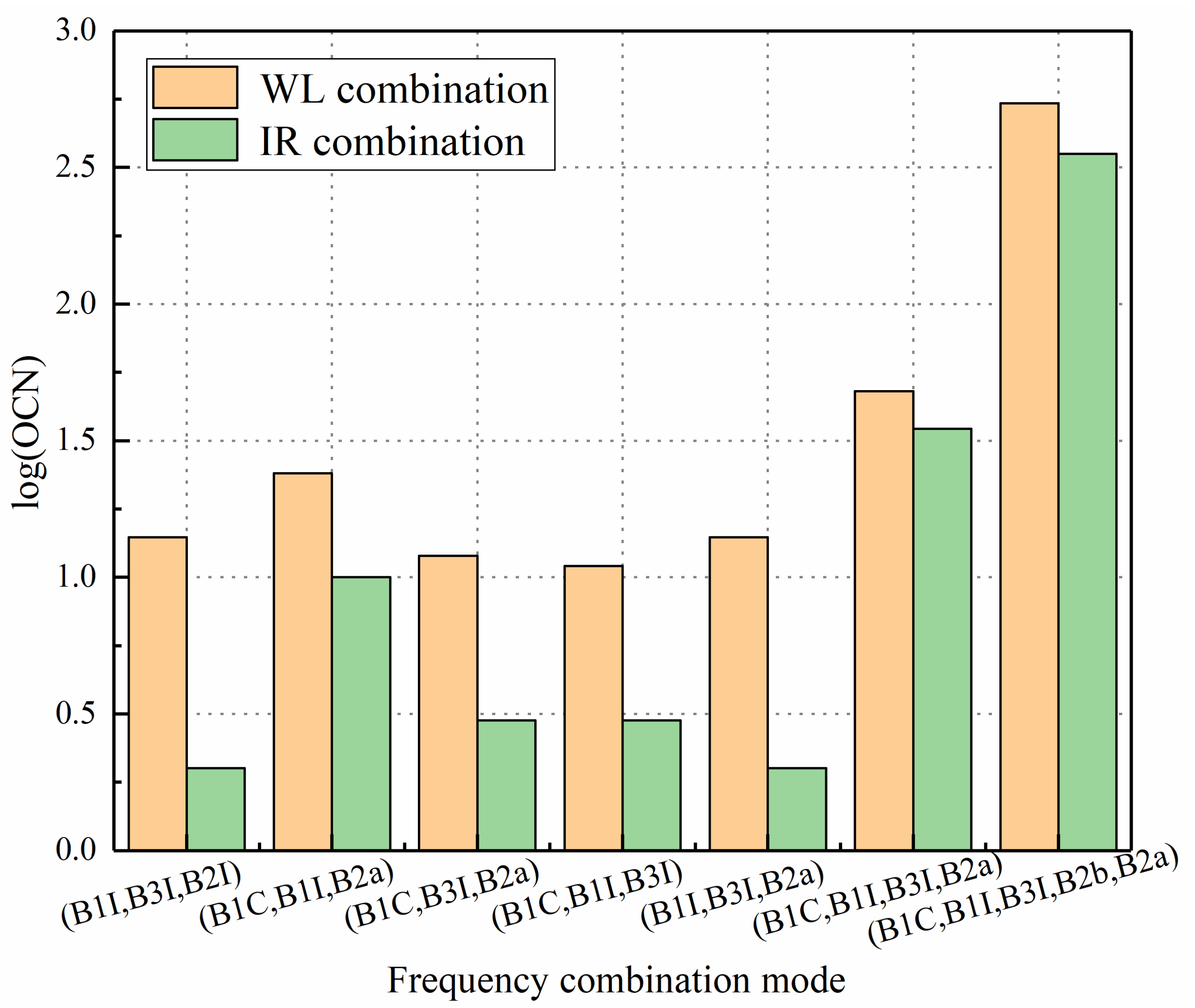
3.1. WL and IR Combinations

Different combination coefficients can produce combined observations with different properties. Generally, combined observations should have the characteristics of long-wavelength, ionospheric-reduced, and noise-reduced. The WL combination selected in this part requires ${\lambda }_c/{\lambda }_{\max }>10$, and ${\lambda }_{\max }$ represents the longest wavelength between several combination frequencies. That is, the wavelength of the combined observation is more than 10 times any frequency wavelength in the combination. It should be noted that only the case where the wavelength is positive is considered in this paper. Theoretically, the combined wavelength can be negative, but only in the numerical sense are the characteristics the same as the positive value. The IR combination requires that ${\mu }_c{}^{\prime }<0.1$. In addition, ${\theta }^{\prime }<10$ is set for all combinations [35]. The high-quality signals of different frequency combinations were obtained by traversal within the range of −10 to 10.

Table 4. WL and IR combinations of BDS-2 TF combination.

a1	a2	a3	S_a	${\mathit{\lambda }}_{\mathit{c}}$	${\mathit{\lambda }}_{\mathit{c}}/{\mathit{\lambda }}_{\mathbf{max}}$	${\mathit{\mu }}_{\mathit{c}}$	${\mathit{\mu }}_{\mathit{c}}{}^{\prime }$	$\mathit{\theta }$	${\mathit{\theta }}^{\prime }$	$\mathit{S}\_\mathit{\eta }$
−1	6	−5	0	20.932	84.286	−8.963	−0.428	164.821	7.874	1
1	−5	4	0	6.371	25.652	0.652	0.102	41.287	6.481	1
0	1	−1	0	4.884	19.667	−1.591	−0.326	6.907	1.414	1
−1	7	−6	0	3.960	15.946	−2.986	−0.754	36.725	9.274	1
1	−4	3	0	2.765	11.132	−0.618	−0.223	14.097	5.099	1
−3	−2	6	1	13.321	53.636	159.400	11.966	93.244	7.000	1
4	−3	−2	−1	12.211	49.167	−144.867	−11.864	65.756	5.385	1
−4	4	1	1	8.140	32.778	93.925	11.538	46.763	5.745	1
3	3	−7	−1	7.712	31.053	−94.797	−12.292	63.125	8.185	1
5	−8	2	−1	4.186	16.857	−49.240	−11.762	40.373	9.644	1
−3	−1	5	1	3.574	14.390	41.601	11.641	21.143	5.916	1
4	−2	−3	−1	3.489	14.048	−42.527	−12.190	18.787	5.385	1
−4	5	0	1	3.053	12.292	34.227	11.212	19.546	6.403	1
3	4	−8	−1	2.990	12.041	−37.732	−12.618	28.211	9.434	1
4	2	−5	1	0.109	0.440	−0.003	−0.025	0.732	6.708	1
5	−3	−1	1	0.107	0.432	0.008	0.077	0.635	5.916	1

,

Table 5. WL and IR combinations of BDS-3 TF combination.

a1	a2	a3	a4	a5	S_a	${\mathit{\lambda }}_{\mathit{c}}$	${\mathit{\lambda }}_{\mathit{c}}/{\mathit{\lambda }}_{\mathbf{max}}$	${\mathit{\mu }}_{\mathit{c}}$	${\mathit{\mu }}_{\mathit{c}}{}^{\prime }$	$\mathit{\theta }$	${\mathit{\theta }}^{\prime }$	$\mathit{S}\_\mathit{\eta }$
(B1C, B1I, B2a)
1	−1	/	/	0	0	20.932	82.143	−1.009	−0.048	29.603	1.414	1
2	1	/	/	−4	−1	48.842	191.667	−602.486	−12.335	223.822	4.583	1
−1	−2	/	/	4	1	36.632	143.750	450.098	12.287	167.867	4.583	1
3	0	/	/	−4	−1	14.653	57.500	−181.452	−12.384	73.263	5.000	1
0	−3	/	/	4	1	13.321	52.273	163.030	12.239	66.603	5.000	1
1	−4	/	/	4	1	8.140	31.944	99.237	12.191	46.763	5.745	1
2	−5	/	/	4	1	5.861	23.000	71.168	12.143	39.317	6.708	1
3	−6	/	/	4	1	4.579	17.969	55.379	12.094	35.763	7.810	1
4	−7	/	/	4	1	3.757	14.744	45.258	12.046	33.814	9.000	1
4	−1	/	/	−4	−1	8.619	33.824	−107.152	−12.432	49.513	5.745	1
5	−2	/	/	−4	−1	6.105	23.958	−76.194	−12.480	40.955	6.708	1
6	−3	/	/	−4	−1	4.727	18.548	−59.217	−12.528	36.916	7.810	1
7	−4	/	/	−4	−1	3.856	15.132	−48.494	−12.576	34.704	9.000	1
−3	−3	/	/	8	2	146.526	575.000	3607.851	24.623	1326.851	9.055	1
1	3	/	/	−3	1	0.110	0.431	0.006	0.053	0.479	4.359	1
2	2	/	/	−3	1	0.109	0.429	0.001	0.005	0.451	4.123	1
3	1	/	/	−3	1	0.109	0.427	−0.005	−0.043	0.474	4.359	1
4	0	/	/	−3	1	0.108	0.424	−0.010	−0.091	0.541	5.000	1
(B1C, B3I, B2a)
1	/	−4	/	3	0	9.768	38.333	2.549	0.261	49.809	5.099	1
−1	/	5	/	−4	0	4.884	19.167	−3.769	−0.772	31.653	6.481	1
0	/	1	/	−1	0	3.256	12.778	−1.663	−0.511	4.605	1.414	1
−2	/	−4	/	7	1	29.305	115.000	370.550	12.645	243.427	8.307	1
3	/	0	/	−4	−1	14.653	57.500	−181.452	−12.384	73.263	5.000	1
−4	/	5	/	0	1	7.326	28.750	85.073	11.612	46.911	6.403	1
4	/	−4	/	−1	−1	5.861	23.000	−71.052	−12.123	33.669	5.745	1
−3	/	1	/	3	1	4.186	16.429	49.705	11.873	18.248	4.359	1
2	/	5	/	−8	−1	3.663	14.375	−48.190	−13.155	35.326	9.644	1
5	/	−8	/	2	−1	3.663	14.375	−43.452	−11.862	35.326	9.644	1
−2	/	−3	/	6	1	2.931	11.500	35.558	12.134	20.514	7.000	1
3	/	1	/	−5	−1	2.664	10.455	−34.352	−12.894	15.761	5.916	1
2	/	−7	/	5	0	1.954	7.667	0.022	0.011	17.254	8.832	1
4	/	0	/	−3	1	0.108	0.424	−0.010	−0.091	0.541	5.000	1
6	/	−7	/	2	1	0.102	0.402	−0.008	−0.080	0.967	9.434	1
(B1C, B1I, B3I)
1	−1	0	/	/	0	20.932	88.571	−1.009	−0.048	29.603	1.414	1
7	−3	−5	/	/	−1	146.526	620.000	−1722.644	−11.757	1334.917	9.110	1
−6	2	5	/	/	1	24.421	103.333	285.930	11.708	196.889	8.062	1
−5	1	5	/	/	1	11.271	47.692	131.424	11.660	80.493	7.141	1
−4	0	5	/	/	1	7.326	31.000	85.073	11.612	46.911	6.403	1
−3	−1	5	/	/	1	5.427	22.963	62.755	11.564	32.106	5.916	1
−2	−2	5	/	/	1	4.310	18.235	49.627	11.516	24.757	5.745	1
−1	−3	5	/	/	1	3.574	15.122	40.982	11.467	21.143	5.916	1
0	−4	5	/	/	1	3.053	12.917	34.858	11.419	19.546	6.403	1
1	−5	5	/	/	1	2.664	11.273	30.293	11.371	19.026	7.141	1
2	−6	5	/	/	1	2.363	10.000	26.759	11.323	19.054	8.062	1
7	−2	−4	/	/	1	0.106	0.448	0.008	0.073	0.879	8.307	1
8	−3	−4	/	/	1	0.105	0.446	0.003	0.025	0.994	9.434	1
(B1I, B3I, B2a)
/	1	−4	/	3	0	18.316	71.875	5.559	0.304	93.392	5.099	1
/	−1	5	/	−4	0	3.960	15.541	−3.188	−0.805	25.665	6.481	1
/	0	1	/	−1	0	3.256	12.778	−1.633	−0.502	4.605	1.414	1
/	1	−3	/	2	0	2.765	10.849	−0.547	−0.198	10.344	3.742	1
/	−4	4	/	1	1	48.842	191.667	572.132	11.714	280.576	5.745	1
/	5	−8	/	2	−1	29.305	115.000	−334.384	−11.410	282.609	9.644	1
/	−3	0	/	4	1	13.321	52.273	160.079	12.017	66.603	5.000	1
/	−2	−4	/	7	1	7.712	30.263	95.018	12.321	64.060	8.307	1
/	2	5	/	−8	−1	5.636	22.115	−72.263	−12.823	54.348	9.644	1
/	3	1	/	−5	−1	4.310	16.912	−53.952	−12.519	25.496	5.916	1
/	4	−3	/	−2	−1	3.489	13.690	−42.616	−12.215	18.787	5.385	1
/	−4	5	/	0	1	3.053	11.979	34.227	11.212	19.546	6.403	1
/	5	−7	/	1	−1	2.931	11.500	−34.908	−11.912	25.379	8.660	1
/	−3	1	/	3	1	2.617	10.268	30.132	11.516	11.405	4.359	1
/	4	0	/	−3	1	0.110	0.433	0.011	0.100	0.552	5.000	1
/	5	−3	/	−1	1	0.106	0.417	−0.010	−0.098	0.628	5.916	1

and

Table 6. WL and IR combinations of BDS-3 QF and FF combinations.

a1	a2	a3	a4	a5	S_a	${\mathit{\lambda }}_{\mathit{c}}$	${\mathit{\lambda }}_{\mathit{c}}/{\mathit{\lambda }}_{\mathbf{max}}$	${\mathit{\mu }}_{\mathit{c}}$	${\mathit{\mu }}_{\mathit{c}}{}^{\prime }$	$\mathit{\theta }$	${\mathit{\theta }}^{\prime }$	$\mathit{S}\_\mathit{\eta }$
(B1C, B1I, B3I, B2a)
1	−1	0	/	0	0	20.932	82.143	−1.009	−0.048	29.603	1.414	1
0	1	−4	/	3	0	18.316	71.875	5.662	0.309	93.392	5.099	1
−5	6	−3	/	2	0	8.140	31.944	0.321	0.039	70.026	8.602	1
−4	5	−3	/	2	0	5.861	23.000	−0.052	−0.009	43.070	7.348	1
−3	4	−3	/	2	0	4.579	17.969	−0.261	−0.057	28.226	6.164	1
4	−3	−4	/	3	0	4.070	15.972	0.473	0.116	28.780	7.071	1
−1	1	1	/	−1	0	3.856	15.132	−1.784	−0.463	7.712	2.000	1
−2	3	−3	/	2	0	3.757	14.744	−0.395	−0.105	19.157	5.099	1
0	0	1	/	−1	0	3.256	12.778	−1.663	−0.511	4.605	1.414	1
−1	2	−3	/	2	0	3.185	12.500	−0.489	−0.153	13.514	4.243	1
6	−5	−4	/	3	0	2.931	11.500	0.058	0.020	27.177	9.274	1
1	−1	1	/	−1	0	2.818	11.058	−1.575	−0.559	5.636	2.000	1
0	1	−3	/	2	0	2.765	10.849	−0.557	−0.202	10.344	3.742	1
1	3	0	/	−3	1	0.110	0.431	0.006	0.053	0.479	4.359	1
2	2	0	/	−3	1	0.109	0.429	0.001	0.005	0.451	4.123	1
3	1	0	/	−3	1	0.109	0.427	−0.005	−0.043	0.474	4.359	1
−2	7	−3	/	−1	1	0.107	0.421	0.000	−0.004	0.851	7.937	1
(B1C, B1I, B3I, B2b, B2a)
1	−1	0	0	0	0	20.932	82.143	−1.009	−0.048	29.603	1.414	1
1	−1	2	−6	4	0	20.932	82.143	0.078	0.004	159.416	7.616	1
−4	5	−3	0	2	0	5.861	23.000	−0.052	−0.009	43.070	7.348	1
−1	2	−4	2	1	0	4.727	18.548	−0.002	0.000	24.101	5.099	1
−3	4	−1	−6	6	0	4.579	17.969	−0.023	−0.005	45.329	9.899	1
2	−1	−5	4	0	0	3.960	15.541	0.031	0.008	26.859	6.782	1
2	−1	−6	7	−2	0	3.960	15.541	−0.072	−0.018	38.395	9.695	1
0	1	−2	−4	5	0	3.856	15.132	0.012	0.003	26.152	6.782	1
3	−2	−3	−2	4	0	3.330	13.068	0.038	0.012	21.582	6.481	1
3	−2	−4	1	2	0	3.330	13.068	−0.048	−0.014	19.418	5.831	1
0	0	1	0	−1	0	3.256	12.778	−1.663	−0.511	4.605	1.414	1
6	−5	−4	0	3	0	2.931	11.500	0.058	0.020	27.177	9.274	1
6	−5	−5	3	1	0	2.931	11.500	−0.018	−0.006	28.713	9.798	1
4	−3	−2	−5	6	0	2.873	11.275	−0.031	−0.011	27.256	9.487	1
2	1	2	4	−8	1	0.112	0.441	2.0 × 10−4	1.8 × 10−3	1.061	9.434	1
2	2	1	−3	−1	1	0.109	0.429	3.4 × 10−3	3.1 × 10−2	0.476	4.359	1
0	4	3	−8	2	1	0.109	0.428	5.0 × 10−5	4.6 × 10−4	1.053	9.644	1
3	1	0	0	−3	1	0.109	0.427	−4.7 × 10−3	−4.3 × 10−2	0.474	4.359	1
1	4	−4	2	−2	1	0.107	0.419	4.8 × 10−4	4.5 × 10−3	0.684	6.403	1
−1	6	−1	−6	3	1	0.107	0.419	−3.8 × 10−6	−3.6 × 10−5	0.972	9.110	1
1	7	1	−2	−5	2	0.055	0.215	9.6 × 10−5	1.8 × 10−3	0.490	8.944	1

list some optimal combinations of different frequency combinations. To distinguish coefficients of different frequencies, a₁~a_n correspond to f₁~f_n in Table 1 respectively; for example, a₅ denotes the combination coefficient corresponding to f₅ (B2a) in cycles. $S\_a={\displaystyle \sum _{i=1}^n{a}_i}$ and $S\_\eta ={\displaystyle \sum _{i=1}^n{\eta }_i}$ represent the sum of the combined coefficients in cycles and meters, respectively.

It can be seen from Table 4, Table 5 and Table 6 that each combination satisfies $S\_\eta =1$, that is, the combined observation can ensure that the geometric distance from the satellite to the receiver remains unchanged. With the increase in the number of combination frequencies, the number of optimal combinations increases significantly. Figure 1 shows the optimal combination number (OCN) of WL and IR combinations under different conditions. The ionospheric delay of the WL combination is related to S_a. Table 4, Table 5 and Table 6 show that ${\mu }_c{}^{\prime }$ is about 12 times that of S_a, the same as in the literature [32,35]. The wavelength of the IR combination fluctuates between 10~12 cm. When the number of frequencies increases, the accuracy of the combined observation is also improved. For instance, the IR combination of five frequencies, ${\mu }_c$ is mostly less than 1 mm, which is about 1/10 times that of the TF combination.

WL and IR combinations are often used in ambiguity resolution. In different application scenarios, the criteria for the selected combination are also different. When the baseline is short, the atmospheric delay correlation between the two stations is strong, and most of the errors can be weakened by single differencing, so combinations with a longer wavelength and small noise should be mainly selected to facilitate the resolution of ambiguity. Such as the WL combinations (−1, 6, −5) and (−3, −2, 6) for (B1I, B3I, B2I), (2, 1, −4) and (−1, −2, 4) for (B1C, B1I, B2a), (1, −1, 0, 0) and (0, 1, −4, 3) for (B1C, B1I, B3I, B2a), (1, −1, 0, 0, 0) and (1, −1, 2, −6, 4) for (B1C, B1I, B3I, B2b, B2a). For long baselines, where the correlation between two stations is weak, combinations with small ionospheric delay and small noise are required. Such as the IR combinations (4, 2, −5) and (5, −3, −1) for (B1I, B3I, B2I), (2, 2, −3) and (3, 1, −3) for (B1C, B1I, B2a), (−2, 7, −3, 1) and (2, 2, 0, −3) for (B1C, B1I, B3I, B2a), (0, 4, 3, −8, 2) and (−1, 6, −1, −6, 3) for (B1C, B1I, B3I, B2b, B2a). The other combinations with relatively large wavelength and small ionospheric delay are suitable for medium-long baselines. Such as (1, −4, 3) and (0, 1, −1) for (B1I, B3I, B2I), (−4, 5, −3, 2) and (−1, 1, 1, −1) for (B1C, B1I, B3I, B2a), (−1, 2, −4, 2, 1) and (0, 1, −2, −4, 5) for (B1C, B1I, B3I, B2b, B2a).

3.2. GF Combinations

The GF combination can eliminate the influence of frequency-independent terms, such as orbit error, receiver clock error, tropospheric delay error, etc., and is often used for cycle slip detection of phase observations. For multi-frequency observations, the GF combination satisfies $f_c=0$. Besides, the combinations with small combined noise and ionospheric delay should also be considered as they can improve the cycle slip detection accuracy. For the GF combination, the cycle slip test quantity can be constructed by making a difference between the epochs of the combined observations, $\vartheta ={\mu }_c{}^{\prime }/(\sqrt{2}{\theta }^{\prime })$ and $\tau =0.01/\vartheta$ are introduced to measure the influence of the residual ionospheric delay on the cycle slip after the difference [8,35]. According to Section 3.1, as the number of combination frequencies and traversal range increases, the optimal combination number will increase sharply, and the traversal duration will also increase significantly. Therefore, considering S_a ≤ 3, for TF and QF/FF, make $a_i$ between [−500,500] and [−50,50], ${\theta }^{\prime }$ less than 500 and 100, and ${\mu }_c{}^{\prime }$ less than 50 and 30, respectively.

Table 7. GF combinations of BDS-2 TF combination.

a1	a2	a3	S_a	${\mathit{\theta }}^{\prime }$	${\mathit{\mu }}_{\mathit{c}}{}^{\prime }$	$\mathit{\vartheta }$	$\mathit{\tau }$
−10	38	−27	1	47.676	9.621	0.143	0.070
40	−211	170	−1	273.900	0.944	0.002	4.102
−50	249	−197	2	321.419	8.677	0.019	0.524
30	−173	143	0	226.446	10.565	0.033	0.303
−60	287	−224	3	368.978	18.297	0.035	0.285
50	−308	259	1	405.518	30.751	0.054	0.186
20	−135	116	1	179.112	20.186	0.080	0.125
0	−59	62	3	85.586	39.427	0.326	0.031

,

Table 8. GF combinations of BDS-3 TF combination.

a1	a2	a3	a4	a5	S_a	${\mathit{\theta }}^{\prime }$	${\mathit{\mu }}_{\mathit{c}}{}^{\prime }$	$\mathit{\vartheta }$	$\mathit{\tau }$
(B1C, B1I, B2a)
−30	25	/	/	7	2	39.674	24.190	0.431	0.023
188	−195	/	/	7	0	270.958	3.074	0.008	1.247
−297	305	/	/	−7	1	425.773	7.484	0.012	0.805
267	−280	/	/	14	1	387.150	16.706	0.031	0.328
−109	110	/	/	0	1	154.858	10.558	0.048	0.207
79	−85	/	/	7	1	116.254	13.632	0.083	0.121
−139	135	/	/	7	3	193.894	34.749	0.127	0.079
49	−60	/	/	14	3	78.721	37.822	0.340	0.029
(B1C, B3I, B2a)
−10	/	5	/	8	3	13.748	36.379	1.871	0.005
−94	/	369	/	−272	3	467.954	0.161	0.000	41.000
97	/	−382	/	282	−3	484.620	1.132	0.002	6.054
−91	/	356	/	−262	3	451.288	1.455	0.002	4.387
−88	/	343	/	−252	3	434.623	2.748	0.004	2.236
−85	/	330	/	−242	3	417.958	4.042	0.007	1.462
−79	/	304	/	−222	3	384.631	6.629	0.012	0.821
−76	/	291	/	−212	3	367.969	7.922	0.015	0.657
3	/	−13	/	10	0	16.673	1.293	0.055	0.182
−49	/	174	/	−122	3	218.085	19.564	0.063	0.158
(B1C, B1I, B3I)
−41	30	14	/	/	3	52.697	35.011	0.470	0.021
143	−150	7	/	/	0	207.360	1.668	0.006	1.758
−252	260	−7	/	/	1	362.151	8.890	0.017	0.576
320	−340	21	/	/	1	467.377	15.562	0.024	0.425
177	−190	14	/	/	1	260.048	13.894	0.038	0.265
211	−230	21	/	/	2	312.829	26.120	0.059	0.169
245	−270	28	/	/	3	365.662	38.347	0.074	0.135
(B1I, B3I, B2a)
/	−10	29	/	−18	1	35.567	9.391	0.187	0.054
/	−65	246	/	−179	2	311.098	1.112	0.003	3.957
/	55	−217	/	161	−1	275.744	8.280	0.021	0.471
/	−75	275	/	−197	3	346.495	10.503	0.021	0.467
/	45	−188	/	143	0	240.454	17.671	0.052	0.192
/	80	−347	/	268	1	445.683	44.733	0.071	0.141
/	35	−159	/	125	1	205.258	27.062	0.093	0.107
/	25	−130	/	107	2	170.218	36.453	0.151	0.066

and

Table 9. GF combinations of BDS-3 QF and FF combinations.

a1	a2	a3	a4	a5	S_a	${\mathit{\theta }}^{\prime }$	${\mathit{\mu }}_{\mathit{c}}{}^{\prime }$	$\mathit{\vartheta }$	$\mathit{\tau }$
(B1C, B1I, B3I, B2a)
−2	−5	4	/	5	2	8.367	24.265	2.051	0.005
−8	5	1	/	3	1	9.950	12.114	0.861	0.012
14	−15	2	/	−1	0	20.640	0.037	0.001	7.795
−39	45	−19	/	13	0	63.844	1.181	0.013	0.764
45	−45	−7	/	7	0	64.405	1.406	0.015	0.648
−25	30	−17	/	12	0	44.249	1.219	0.019	0.514
31	−30	−9	/	8	0	44.788	1.368	0.022	0.463
−11	15	−15	/	11	0	26.306	1.256	0.034	0.296
17	−15	−11	/	9	0	26.758	1.331	0.035	0.284
20	−15	−24	/	19	0	39.522	2.624	0.047	0.213
(B1C, B1I, B3I, B2b, B2a)
0	0	1	−3	2	0	3.742	0.026	0.005	2.037
1	0	−5	2	2	0	5.831	0.414	0.050	0.199
−27	30	−22	41	−22	0	65.406	0.001	1 × 10−5	693.743
−1	0	21	−50	30	0	61.984	0.002	2 × 10−5	519.787
41	−45	23	−38	19	0	77.717	0.010	9 × 10−5	108.367
42	−45	2	12	−11	0	63.702	0.008	9 × 10−5	106.540
−13	15	−21	44	−25	0	58.275	0.013	2 × 10−4	64.341
1	0	−20	47	−28	0	58.258	0.024	3 × 10−4	33.927
14	−15	1	3	−3	0	20.976	0.011	4 × 10−4	25.850
28	−30	3	3	−4	0	41.449	0.049	0.001	11.982
−14	15	1	−9	7	0	23.495	0.040	0.001	8.211
14	−15	3	−3	1	0	20.976	0.063	0.002	4.678
14	−15	5	−9	5	0	23.495	0.115	0.003	2.880
1	0	−12	23	−12	0	28.601	0.232	0.006	1.743
1	0	−11	20	−10	0	24.940	0.258	0.007	1.367
1	0	−10	17	−8	0	21.307	0.284	0.009	1.061

list some GF combinations of TF, QF, and FF. It should be noted that some of the combinations of different frequencies are repeated with other combinations, which are not listed again in the table. For example, (B1C, B1I, B3I) and (B1C, B1I, B2a), the characteristics of combination (110, −109, 0) are consistent. Similar to Figure 1, as the combination frequency increases, more combinations are available, and ${\mu }_c{}^{\prime }$ and ${\theta }^{\prime }$ are smaller. Besides, ${\theta }^{\prime }$ of QF and FF combinations are mostly smaller than the minimum ${\theta }^{\prime }$ of different TF combinations.

The combined observations after the difference between adjacent epochs can be considered to be mainly composed of ionospheric delay variation and cycle slip. Therefore, in cycle slip detection, the corresponding combinations should be selected according to different cases. When the ionospheric delay variation between epochs is in different orders of magnitude, the combination can be selected according to $\tau$. If the ionospheric delay change between adjacent epochs is less than 1 cm, (0, −59, 62) and (−10, 38, −27) for (B1I, B3I, B2I), (−30, 25, 7) and (49, −60, 14) for (B1C, B1I, B2a), (−2, −5, 4, 5) and (−8, 5, 1, 3) for (B1C, B1I, B3I, B2a), (0, 0, 1, −3, 2) and (1, 0, −5, 2, 2) for (B1C, B1I, B3I, B2b, B2a) can be selected. If the ionospheric delay change between adjacent epochs is less than 1 dm, (20, −135, 116) and (30, −173, 143) for (B1I, B3I, B2I), (79, −85, 7) and (−109, 110, 0) for (B1C, B1I, B2a), (−11, 15, −15, 11) and (17, −15, −11, 9) for (B1C, B1I, B3I, B2a) can be selected. If the ionospheric delay change between adjacent epochs is less than 1 m, (40, −211, 170) for (B1I, B3I, B2I), (188, −195, 7) for (B1C, B1I, B2a), (14, −15, 2, −1) for (B1C, B1I, B3I, B2a) can be selected. For TF and QF, most linear combinations can be applied to the ionospheric delay variation between epochs at the centimeter-level or decimeter-level. For the FF combination, 14,765 combinations can be obtained under the above restrictions, among which 410 and 2362 combinations can satisfy the ionospheric delay variation below meter-level and decimeter-level, respectively. When the ionosphere changes violently between epochs, such as tens of meters, the combination of TF or QF cannot be used, but the combination of FF can still be used, such as (−27, 30, −22, 41, −22), (1, 0, 21, −50,30), (41, −45, 23, −38, 19) and (42, −45, 2, 12, −11). If the ionosphere changes in the meter level, the combination of (−13, 15, −21, 44, −25), (1, 0, −20, 47, −28), and (14, −15, 1, 3, −3), etc. can be selected.

3.3. IF Combinations

The IF combination can eliminate the effects of ionospheric delays and is often used in precise positioning [8,35]. If only ${\mu }_c=0$ and ${\mu }_c{}^{\prime }=0$ are considered, we can get $a_1/f_1+a_2/f_2+a_3/f_3+a_4/f_4+a_5/f_5=0$. Similar to Section 3.1, in the case where only positive values of wavelength are considered, the combination with small noise is searched. For TF, QF and FF, make $a_i$ between [−1000,1000], [−300,300] and [−200,200], and ${\theta }^{\prime }$ less than 1000, 500, and 300, respectively. The IF combinations of different frequency combinations are shown in

Table 10. IF combinations of BDS-2 TF combination.

a1	a2	a3	${\mathit{\eta }}_1$	${\mathit{\eta }}_2$	${\mathit{\eta }}_3$	${\mathit{\lambda }}_{\mathit{c}}$	${\mathit{\theta }}^{\prime }$	$\mathit{\theta }$	$\mathsf{\Omega }$	S_a	$\mathit{S}\_\mathit{\eta }$
0	62	−59	0.000	10.590	−9.590	40.365	85.586	3.455	14.286	3	1
763	−620	0	2.944	−1.944	0.000	0.741	983.142	0.728	3.527	143	1
763	−558	−59	2.891	−1.718	−0.173	0.728	947.108	0.689	3.367	146	1
763	−186	−413	2.609	−0.517	−1.092	0.657	887.318	0.583	2.875	164	1
763	−124	−472	2.567	−0.339	−1.228	0.646	905.720	0.585	2.865	167	1
763	−248	−354	2.652	−0.700	−0.951	0.667	876.920	0.585	2.903	161	1
763	−310	−295	2.696	−0.890	−0.806	0.679	874.811	0.594	2.952	158	1
763	−62	−531	2.526	−0.167	−1.360	0.636	931.651	0.592	2.874	170	1

and

Table 11. IF combinations of BDS-3 TF combination.

a1	a2	a3	a4	a5	${\mathit{\eta }}_1$	${\mathit{\eta }}_2$	${\mathit{\eta }}_3$	${\mathit{\eta }}_4$	${\mathit{\eta }}_5$	${\mathit{\lambda }}_{\mathit{c}}$	${\mathit{\theta }}^{\prime }$	$\mathit{\theta }$	$\mathsf{\Omega }$	S_a	$\mathit{S}\_\mathit{\eta }$
(B1C, B1I, B2a)
110	−109	/	/	0	55.25	−54.25	/	/	0.00	95.58	154.86	14.80	77.43	1	1
154	0	/	/	−115	2.26	0.00	/	/	−1.26	2.79	192.20	0.54	2.59	39	1
44	109	/	/	−115	0.67	1.63	/	/	−1.30	2.88	164.44	0.47	2.19	38	1
242	218	/	/	−345	1.21	1.08	/	/	−1.29	0.95	474.46	0.45	2.07	115	1
286	327	/	/	−460	1.07	1.22	/	/	−1.29	0.71	632.71	0.45	2.07	153	1
(B1C, B3I, B2a)
154	/	−496	/	345	12.57	/	−32.59	/	21.03	15.53	623.50	9.68	40.77	3	1
77	/	−186	/	115	5.87	/	−11.42	/	6.55	14.51	231.84	3.37	14.42	6	1
77	/	−62	/	0	2.84	/	−1.84	/	0.00	7.03	98.86	0.69	3.39	15	1
385	/	−62	/	−230	2.36	/	−0.31	/	−1.05	1.17	452.74	0.53	2.60	93	1
616	/	−124	/	−345	2.38	/	−0.39	/	−1.00	0.74	716.84	0.53	2.61	147	1
693	/	−62	/	−460	2.31	/	−0.17	/	−1.15	0.64	834.08	0.53	2.59	171	1
(B1C, B1I, B3I)
187	−109	−62	/	/	6.43	−3.72	−1.72	/	/	6.55	225.15	1.47	7.62	16	1
297	−218	−62	/	/	9.56	−6.95	−1.61	/	/	6.13	373.60	2.29	11.93	17	1
121	109	−186	/	/	1.53	1.36	−1.89	/	/	2.40	247.22	0.59	2.79	44	1
440	327	−620	/	/	1.66	1.22	−1.89	/	/	0.72	827.60	0.59	2.80	147	1
407	436	−682	/	/	1.40	1.49	−1.89	/	/	0.66	906.02	0.59	2.79	161	1
44	109	−124	/	/	0.84	2.07	−1.91	/	/	3.65	170.86	0.62	2.94	29	1
(B1I, B3I, B2a)
/	0	124	/	−115	/	0.00	7.15	/	−6.15	13.62	169.12	2.30	9.43	9	1
/	763	−620	/	0	/	2.94	−1.94	/	0.00	0.74	983.14	0.73	3.53	143	1
/	763	−124	/	−460	/	2.42	−0.32	/	−1.10	0.61	899.52	0.55	2.67	179	1
/	763	−248	/	−345	/	2.53	−0.67	/	−0.86	0.64	873.33	0.56	2.76	170	1
/	763	0	/	−575	/	2.31	0.00	/	−1.31	0.58	955.40	0.56	2.66	188	1
(B1C, B1I, B3I, B2a)
187	−109	−186	/	115	12.38	−7.15	−9.92	0.00	5.69	12.60	307.69	3.88	18.31	7	1
110	−109	124	/	−115	6.89	−6.77	6.26	0.00	−5.38	11.92	229.31	2.73	12.71	10	1
121	109	−62	/	−115	1.30	1.16	−0.54	0.00	−0.92	2.04	208.78	0.43	2.04	53	1
165	218	−62	/	−230	1.04	1.36	−0.31	0.00	−1.08	1.19	362.62	0.43	2.04	91	1
(B1C, B1I, B3I, B2b, B2a)
0	0	62	−177	115	0.00	0.00	284.74	−773.56	489.81	1085.38	220.00	238.78	958.85	0	1
110	−109	−62	177	−115	60.59	−59.49	−27.50	74.70	−47.30	104.81	269.03	28.20	125.63	1	1
110	−109	62	−177	115	50.78	−49.86	23.05	−62.61	39.64	87.85	269.03	23.63	105.29	1	1
121	109	0	−59	−115	1.24	1.10	0.00	−0.46	−0.88	1.94	207.91	0.40	1.93	56	1
198	109	−62	−59	−115	1.58	0.86	−0.40	−0.36	−0.69	1.52	267.65	0.41	2.00	71	1
198	109	0	−118	−115	1.53	0.83	0.00	−0.70	−0.66	1.47	279.70	0.41	1.99	74	1
77	0	0	−59	0	2.42	0.00	0.00	−1.42	0.00	5.99	97.01	0.58	2.81	18	1

. As in Section 3.2, there are duplicate combinations that are not listed again in the table but can still be used optionally. In addition, $\mathsf{\Omega }=\sqrt{{\eta }_1{}^2+{\eta }_2{}^2+\cdots +{\eta }_n{}^2}$ is defined to represent the coefficient amplification factor of the IF combination in meters. Since the combined wavelengths are small, the units of ${\lambda }_c$ in Table 10 and Table 11 are set to millimeters, while the units of $\theta$ remain in meters.

It can be seen from Table 10 and Table 11 that ${\theta }^{\prime }$ of IF combinations are relatively large, and ${\lambda }_c$ are very small, mostly in the millimeter and sub-millimeter levels. Therefore, it is generally not suitable for AR. It is worth noting that there are two special combinations in the FF combinations, (0, 0, 62, −177, 115) and (110, −109, −62, 177, −115), which have wavelengths of 1.085m and 0.105m respectively, far exceeding those of most IF combinations and may be considered for long-baseline AR. Both $\theta$ and $\mathsf{\Omega }$ IF combinations are small, which can be used to improve positioning accuracy. As the number of frequencies increases, both $\theta$ and $\mathsf{\Omega }$ become smaller. Such as (763, −186, −413) and (763, −124, −472) of (B1I, B3I, B2I), compared to the (B1I, B3I) combination (763, −620), $\theta$ and $\mathsf{\Omega }$ are reduced by 20.022%, 19.670% and 18.508%, 18.768% respectively. Compared with (154, −115) of (B1C, B2a), $\theta$ and $\mathsf{\Omega }$ decreased by 24.746%, 24.110% and 25.428%, 22.558%, respectively, in the combination of (121, 109, 0, −59, −115) and (198, 109, −62, −59, −115) of (B1C, B1I, B3I, B2b, B2a). It should be noted that, compared to QF combination, FF combination can only improve the accuracy of observations by about 5%, which is not as obvious as their effect on DF and TF combinations. The $\theta$ and $\mathsf{\Omega }$ of the BDS-3 TF combination in Table 3 are better than the BDS-2 TF combination, except (B1I, B3I, B2a). The improvement of the measurement accuracy of the multi-frequency combinations also means that the BDS-3 positioning accuracy will be further improved than BDS-2. Figure 2 shows the optimal combination of different frequency combination modes.

4. Optimal IF Real Combinations

Several special carrier-phase integer linear combination models are introduced in Section 3, and Section 4 will focus on studying carrier-phase or pseudorange optimal IF real combinations. The optimal IF real combination has a unique solution that minimizes $\mathsf{\Omega }$, and the combination coefficient applies to both carrier-phase and pseudorange observation. Based on the principle of minimum combined noise, a simpler derivation method of IF combined coefficient based on the LS principle is proposed in this section. LS method has the property of optimal estimation, which can obtain the parameter solution with minimum noise. In this section, the derivation process of GBIF and GFIF combinations considering the first-order and second-order ionospheric delay is introduced in detail, and the generalized analytical expressions of multi-frequency GBIF and GFIF combinations considering only the first-order ionosphere are given. Then, the characteristics of different frequency combinations are compared and analyzed.

4.1. Optimal GBIF Real Combination

GBIF combination is one of the commonly used function models of PPP, and as the frequency increases, the number of PPP models based on the GBIF combination also increase. For example, FF observations can directly form a FF GBIF combination, or a TF and a DF GBIF combination or four DF GBIF combinations, etc. Therefore, it is meaningful to generalize the unified analytical expression of multi-frequency GBIF combinations for applying multi-frequency PPP. The carrier-phase observations are taken as an example, and the coefficient expression for the multi-frequency GBIF combination is derived.

(1) GBIF_1 mode: GBIF combination without first-order ionospheric delay

Taking the FF observations as an example, to ensure that the geometric distance term of the combined observations remains unchanged and the first-order ionospheric delay term is eliminated, the combination coefficient relationship can be obtained from Equation (3) as [14]:

$$\left\{\begin{array}{l}{\eta }_1+{\eta }_2+{\eta }_3+{\eta }_4+{\eta }_5=1\\ {\eta }_1+{\eta }_2{\mu }_2^{}+{\eta }_3{\mu }_3^{}+{\eta }_4{\mu }_4^{}+{\eta }_5{\mu }_5^{}=0\\ {\eta }_1^2+{\eta }_2^2+{\eta }_3^2+{\eta }_4^2+{\eta }_5^2=\min \end{array}\right.$$

(9)

Equation (9) is generally solved by the lagrange multiplier method, but this method requires much calculation, and additional parameters will be introduced. In this work, we will start with the basic meaning of the parameters of the observation model. According to the properties of the combined observations, a simpler, more convenient method for deriving the GBIF combination coefficient expression is given.

On the premise that only ${\rho }^{*}$ and $I_{1\_1}$ are considered, Equation (2) can be simplified as:

$$\underset{\mathit{Y}}{\underbrace{\left[\begin{array}{c}{L}_1\\ L_2\\ L_3\\ L_4\\ L_5\end{array}\right]}}=\underset{\mathit{B}}{\underbrace{\left[\begin{array}{cc}1& -1\\ 1& -{\mu }_2\\ 1& -{\mu }_3\\ 1& -{\mu }_4\\ 1& -{\mu }_5\end{array}\right]}}\underset{\mathit{X}}{\underbrace{\left[\begin{array}{l}{\rho }^{\ast }\\ \\ \\ \\ I_{1\_1}\end{array}\right]}}$$

(10)

Assuming that the weight matrix of the phase observations is P, then the solution of the parameter X can be obtained by the LS method as:

$$\mathit{X}={({\mathit{B}}^T\mathit{P}\mathit{B})}^{-1}{\mathit{B}}^T\mathit{P}\mathit{Y}$$

(11)

To ensure that the geometric distance of the combined observations remains unchanged and eliminate the first-order ionospheric delay, $\mathbf{\Theta }$ can be defined as a variable control matrix to control the result of X. When $\mathbf{\Theta }=[\begin{array}{cc}1& 0]\end{array}$, Equation (12) can make the coefficients of ${\rho }^{*}$ and $I_{1\_1}$ be 1 and 0, respectively.

$$\stackrel{⌢}{\mathit{X}}=\mathbf{\Theta }\mathit{X}=\mathbf{\Theta }{({\mathit{B}}^T\mathit{P}\mathit{B})}^{-1}{\mathit{B}}^T\mathit{P}\mathit{Y}$$

(12)

According to Equation (3), the combined observation can be expressed as:

$$L_c=\left[\begin{array}{ccccc}{\eta }_1& {\eta }_2& {\eta }_3& {\eta }_4& {\eta }_5\end{array}\right]\left[\begin{array}{c}{L}_1\\ L_2\\ L_3\\ L_4\\ L_5\end{array}\right]$$

(13)

By substituting Equation (12) into (13), the combined coefficient matrix $\mathit{\eta }=\left[\begin{array}{ccccc}{\eta }_1& {\eta }_2& {\eta }_3& {\eta }_4& {\eta }_5\end{array}\right]$ can be expressed as:

$$\mathit{\eta }=\mathbf{\Theta }{({\mathit{B}}^T\mathit{P}\mathit{B})}^{-1}{\mathit{B}}^T\mathit{P}$$

(14)

And then, combined with Equations (10) and (14), the FF combination coefficient in GBIF_1 mode can be written as:

$$\left\{\begin{array}{c}{\eta }_1=\left({\mu }_2^2+{\mu }_3^2+{\mu }_4^2+{\mu }_5^2-{\mu }_2-{\mu }_3-{\mu }_4-{\mu }_5\right)/M_5\hfill \\ {\eta }_2=\left({\mu }_3^2+{\mu }_4^2+{\mu }_5^2-{\mu }_2{\mu }_3-{\mu }_2{\mu }_4-{\mu }_2{\mu }_5-{\mu }_2+1\right)/M_5\hfill \\ {\eta }_3=\left({\mu }_2^2+{\mu }_4^2+{\mu }_5^2-{\mu }_2{\mu }_3-{\mu }_3{\mu }_4-{\mu }_3{\mu }_5-{\mu }_3+1\right)/M_5\hfill \\ {\eta }_4=\left({\mu }_2^2+{\mu }_3^2+{\mu }_5^2-{\mu }_2{\mu }_4-{\mu }_3{\mu }_4-{\mu }_4{\mu }_5-{\mu }_4+1\right)/M_5\hfill \\ {\eta }_5=\left({\mu }_2^2+{\mu }_3^2+{\mu }_4^2-{\mu }_2{\mu }_5-{\mu }_3{\mu }_5-{\mu }_4{\mu }_5-{\mu }_5+1\right)/M_5\hfill \end{array}\right.$$

(15)

$$M_5={\displaystyle \sum _{i=2}^4{\displaystyle \sum _{j=i+1}^5{({\mu }_i^{}-{\mu }_j^{})}^2+{\displaystyle \sum _{k=2}^5{({\mu }_k^{}-1)}^2}}}$$

(16)

Other methods are used to solve Equation (9) and compared with Equation (15), which can also easily prove that the results are consistent. Similarly, the solution of DF, TF, and QF shows that when the total number of frequencies is n (n ≥ 2), ${\eta }_i$ can be expressed as:

$$\left\{\begin{array}{l}{\eta }_1={\displaystyle \sum _{i=2}^n({\mu }_i^2-}{\mu }_i^{})/M_n\\ {\eta }_m=({\displaystyle \sum _{i=2}^n{\mu }_i^2}-{\displaystyle \sum _{i=2}^n{\mu }_m^{}{\mu }_i^{}}-{\mu }_m^{}+1)/M_n\begin{array}{cc}& (m=2,3,\cdots ,n)\end{array}\end{array}\right.$$

(17)

$$M_n={\displaystyle \sum _{i=2}^{n-1}{\displaystyle \sum _{j=i+1}^n{({\mu }_i^{}-{\mu }_j^{})}^2+{\displaystyle \sum _{k=2}^n{({\mu }_k^{}-1)}^2}}}$$

(18)

(2) GBIF_2 mode: GBIF combination without first-order and second-order ionospheric delay

Compared with the first-order ionospheric delay, the impact of higher-order ionospheric delay is relatively small. However, in some cases, the second-order ionospheric delay still needs to be considered [56]. Based on the above principles, the combined coefficient expression for simultaneously eliminating the first-order and second-order ionospheric delays can be derived.

When the second-order ionospheric delay is considered, Equation (1) can be simplified as:

$$L_i={\rho }^{\ast }-{\mu }_i{I}_{1\_1}-{\nu }_i{I}_{1\_2}/2+{\lambda }_i{N}_i+{\epsilon }_i$$

(19)

Similar to Equation (10), Equation (19) can be written as:

$$\underset{\mathit{Y}}{\underbrace{\left[\begin{array}{c}{L}_1\\ L_2\\ L_3\\ L_4\\ L_5\end{array}\right]}}=\underset{\mathit{B}}{\underbrace{\left[\begin{array}{cc}1& \begin{array}{cc}-1& -1\end{array}\\ 1& \begin{array}{cc}-{\mu }_2& -{\nu }_2\end{array}\\ 1& \begin{array}{cc}-{\mu }_3& -{\nu }_3\end{array}\\ 1& \begin{array}{cc}-{\mu }_4& -{\nu }_4\end{array}\\ 1& \begin{array}{cc}-{\mu }_5& -{\nu }_5\end{array}\end{array}\right]}}\underset{\mathit{X}}{\underbrace{\left[\begin{array}{l}{\rho }^{\ast }\\ \\ I_{1\_1}\\ \\ I_{1\_2}\end{array}\right]}}$$

(20)

It should be noted that the coefficient of $I_{1\_2}$ in Equation (20) is omitted because $I_{1\_2}$ is finally eliminated, so it will not affect the result. The processing involved in the following is the same.

According to the LS principle, $\mathit{X}={({\mathit{B}}^T\mathit{P}\mathit{B})}^{-1}{\mathit{B}}^T\mathit{P}\mathit{Y}$ can also be obtained. In this case, the variable control matrix $\mathbf{\Theta }=[\begin{array}{cc}1& \begin{array}{cc}0& 0\end{array}]\end{array}$ can be defined to ensure that the coefficient of the geometric distance term is 1, while the first-order and second-order ionospheric coefficients are 0. Finally, the coefficient matrix $\mathit{\eta }=\mathbf{\Theta }{({\mathit{B}}^T\mathit{P}\mathit{B})}^{-1}{\mathit{B}}^T\mathit{P}$ can also be obtained.

Since the coefficient expression in GBIF_2 mode is complex, only the TF combination expression is given:

$$\left\{\begin{array}{l}{\eta }_1=-({\mu }_2{\nu }_3-{\mu }_3{\nu }_2)/(({\mu }_2-{\mu }_3)-({\nu }_2-{\nu }_3)-({\mu }_2{\nu }_3-{\mu }_3{\nu }_2))\\ {\eta }_2=-({\mu }_3-{\nu }_3)/(({\mu }_2-{\mu }_3)-({\nu }_2-{\nu }_3)-({\mu }_2{\nu }_3-{\mu }_3{\nu }_2))\\ {\eta }_3=({\mu }_2-{\nu }_2)/(({\mu }_2-{\mu }_3)-({\nu }_2-{\nu }_3)-({\mu }_2{\nu }_3-{\mu }_3{\nu }_2))\end{array}\right.$$

(21)

Table 12. GBIF real combination of BDS-2.

Frequency Number	B1I	B3I	B2I	Ω
GBIF_1 mode
DF	2.944	1.944	/	3.527
	2.487	/	−1.487	2.898
	/	10.590	−9.590	14.286
TF	2.566	−0.338	−1.229	2.865
GBIF_2 mode
QF	9.100	−28.157	20.057	35.748

and

Table 13. GBIF real combination of BDS-3.

Frequency Number	B1C	B1I	B3I	B2b	B2a	Ω
GBIF_1 mode
DF	/	2.944	−1.944	/	/	3.527
	55.251	−54.251	/	/	/	77.433
	2.844	/	−1.844	/	/	3.389
	2.422	/	/	−1.422		2.809
	2.261	/	/	/	−1.261	2.588
	/	2.314	/	/	−1.314	2.662
	/		7.148	/	−6.148	9.429
TF	1.503	1.388	−1.891	/	/	2.786
	1.172	1.115	/	/	−1.287	2.067
	2.290	/	−0.094	/	−1.196	2.586
	/	2.343	−0.089	/	−1.254	2.659
QF	1.224	1.171	−0.336	/	−1.058	2.025
FF	1.216	1.170	−0.123	−0.520	−0.742	1.919
GBIF_2 mode
TF	201.948	−206.108	5.161	/	/	288.600
	158.661	−160.121	/	/	2.460	225.428
	7.943	/	−17.968	/	11.025	22.528
	/	8.438	−18.915	/	11.477	23.679
QF	5.532	2.561	−18.256	/	11.162	22.249
FF	5.495	2.555	−17.629	−1.370	11.949	22.184

list the coefficients of the GBIF combination calculated by the LS method. It is clear that the results are the same as the literature [14,15,40,41]. The definition of $\mathsf{\Omega }$ in the tables is the same as that in Section 3.3.

Compared with Section 3.3, it can be found that in GBIF_1 mode, the optimal real coefficients of the DF combination in meters can find the corresponding integer coefficients in cycles, such as the combination (2.944, −1.944) in Table 12 corresponds to the combination (763, −620,0) in Table 10. This shows that when the combined coefficients are rational numbers, the combined ambiguity can also maintain integer characteristics. In addition, the combination coefficients of TF, QF, and FF are smaller than the corresponding frequency combinations in Table 10 and Table 11, which indicates that under the restrictions of Section 3.3, the best IF combination has not been found, which also reflects that the corresponding integer coefficient will be relatively large. The corresponding integer coefficient in cycles can also be derived from the real coefficient in meters. Still, the above has shown that the real coefficient can maintain the integer characteristic of ambiguity, so the corresponding integer coefficient combinations in Table 12 and Table 13 are not derived here. The noise of the BDS-2 TF combination is 2.865, which is smaller than the DF combinations. However, compared with Table 10, it can be found that it is only slightly better than the combination of (763, −124, −472), ${\mathsf{\Omega }}_{TF\_GBIF\_1}-{\mathsf{\Omega }}_{(763,-124,-472)}=-6\times {10}^{-7}$. Therefore, in some application scenarios, the optimal combination can be replaced by (763, −124, −472). Similarly, for each combination in Table 13, the corresponding or approximate integer combination can also be found in Table 10.

For BDS-3, the noise of the (B1I, B3I) combination is higher than other combinations except (B1C, B1I) and (B3I, B2a) in GBIF_1 mode, which is because the difference between the two frequencies is small. The minimum noise of the DF combination is ${\mathsf{\Omega }}_{(B1C,B2a)}=2.588$, compared with the combination of (B1I, B3I), the noise is reduced by 26.624%, which also shows that the combination of the new BDS-3 signal should have a better performance in precise positioning. The optimal combination of TF is ${\mathsf{\Omega }}_{(B1C,B1I,B2a)}=2.067$, and the combined noises of QF and FF are 2.025 and 1.919, respectively. In GBIF_ 2 mode, the combined noise of TF (B1C, B3I, B2a), QF, and FF is 22.528, 22.249, and 22.184, respectively. It can be seen that as the number of combined frequencies increases, the GBIF combined noise also becomes smaller. In addition, compared with the GBIF_1 mode, the combination coefficient of GBIF_2 mode is obviously larger, which also leads to the increase of noise by about 10 times. It is worth noting that (B1C, B1I, B2a) is the best TF combination in GBIF_1 mode, but its combined noise increases 109 times in GBIF_2 mode, which also indicates that the optimal frequency combination in GBIF_1 mode does not apply to GBIF_2 mode. Another point to note is that the B3I frequency has a small contribution to TF (B1C, B3I, B2a), (B1I, B3I, B2a), QF, and FF combined observations in GBIF_1 mode but has a larger contribution to the four combinations in GBIF_2 mode.

4.2. Optimal GFIF Real Combination

In general, the GFIF combination can be obtained by the linear combination of the GBIF combinations in Section 4.1. To derive the general analytical expression of multi-frequency GFIF combination, the coefficients are solved directly in this part. It can be seen from Equation (12) that when the variable control matrix $\mathsf{\Theta }=[\begin{array}{cc}0& 0]\end{array}$, the combination coefficients are all 0. Therefore, the lagrange multiplier method is used to derive the analytical expression of the optimal coefficients of the multi-frequency GFIF combination.

(1) GFIF_1 mode: GFIF combination without first-order ionospheric delay

Similar to the GBIF model, the FF observations are taken as an example, and the relationship between the coefficients of the GFIF_1 mode can be obtained as follows:

$$\left\{\begin{array}{l}{\eta }_1+{\eta }_2+{\eta }_3+{\eta }_4+{\eta }_5=0\\ {\eta }_1+{\eta }_2{\mu }_2^{}+{\eta }_3\cdot {\mu }_3^{}+{\eta }_4\cdot {\mu }_4^{}+{\eta }_5\cdot {\mu }_5^{}=0\\ {\eta }_1^2+{\eta }_2^2+{\eta }_3^2+{\eta }_4^2+{\eta }_5^2=\min \end{array}\right.$$

(22)

It can be seen from Equation (22) that when ${\eta }_1={\eta }_2={\eta }_3={\eta }_4={\eta }_5=0$, the optimal solution can be obtained, but it will make the combined observations meaningless. Therefore, ${\eta }_1$ is set to 1 to prevent the solution results from being all 0, which will not affect the relative relationship between the coefficients [57]. The expression of each frequency coefficient is given by Equation (23):

$$\left\{\begin{array}{c}{\eta }_1=1\hfill \\ {\eta }_2=-\left({\mu }_3^2+{\mu }_4^2+{\mu }_5^2-{\mu }_2{\mu }_3-{\mu }_2{\mu }_4-{\mu }_2{\mu }_5-{\mu }_3-{\mu }_4-{\mu }_5+3{\mu }_2\right)/M_5^{\prime }\hfill \\ {\eta }_3=-\left({\mu }_2^2+{\mu }_4^2+{\mu }_5^2-{\mu }_2{\mu }_3-{\mu }_3{\mu }_4-{\mu }_3{\mu }_5-{\mu }_2-{\mu }_4-{\mu }_5+3{\mu }_3\right)/M_5^{\prime }\hfill \\ {\eta }_4=-\left({\mu }_2^2+{\mu }_3^2+{\mu }_5^2-{\mu }_2{\mu }_4-{\mu }_3{\mu }_4-{\mu }_4{\mu }_5-{\mu }_2-{\mu }_3-{\mu }_5+3{\mu }_4\right)/M_5^{\prime }\hfill \\ {\eta }_5=-\left({\mu }_2^2+{\mu }_3^2+{\mu }_4^2-{\mu }_2{\mu }_5-{\mu }_3{\mu }_5-{\mu }_4{\mu }_5-{\mu }_2-{\mu }_3-{\mu }_4+3{\mu }_5\right)/M_5^{\prime }\hfill \end{array}\right.$$

(23)

$$M_5^{\prime }={\displaystyle \sum _{i=2}^4{\displaystyle \sum _{j=i+1}^5{({\mu }_i^{}-{\mu }_j^{})}^2}}$$

(24)

Similarly, the solution of TF and QF shows that when the total number of frequencies is n (n > 2), ${\eta }_i$ can be expressed as:

$$\left\{\begin{array}{l}{\eta }_1=1\\ {\eta }_m=-({\displaystyle \sum _{i=2}^n({\mu }_i^2}-{\mu }_m^{}{\mu }_i^{}-{\mu }_i^{})+(n-1){\mu }_m^{})/M_m^{\prime }\begin{array}{cc}& (m=2,3,\cdots ,n)\end{array}\end{array}\right.$$

(25)

$$M_n^{\prime }={\displaystyle \sum _{i=2}^{n-1}{\displaystyle \sum _{j=i+1}^n{({\mu }_i^{}-{\mu }_j^{})}^2}}$$

(26)

In GFIF_1 mode, the TF combination of BDS-2 carrier-phase or pseudorange observations can be expressed as:

$$\left\{\begin{array}{l}{P}_c=P_1-4.256P_2+3.256P_3\\ L_c=L_1-4.256L_2+3.256L_3\end{array}\right.\begin{array}{cc}& \mathsf{\Omega }=5.453\end{array}$$

(27)

(2) GFIF_2 mode: GFIF combination without first-order and second-order ionospheric delay

When considering both the first-order and second-order ionospheric delays, Equation (22) needs to be modified as:

$$\left\{\begin{array}{l}{\eta }_1+{\eta }_2+{\eta }_3+{\eta }_4+{\eta }_5=0\\ {\eta }_1+{\eta }_2{\mu }_2^{}+{\eta }_3\cdot {\mu }_3^{}+{\eta }_4\cdot {\mu }_4^{}+{\eta }_5\cdot {\mu }_5^{}=0\\ {\eta }_1+{\eta }_2{\nu }_2^{}+{\eta }_3\cdot {\nu }_3^{}+{\eta }_4\cdot {\nu }_4^{}+{\eta }_5\cdot {\nu }_5^{}=0\\ {\eta }_1^2+{\eta }_2^2+{\eta }_3^2+{\eta }_4^2+{\eta }_5^2=\min \end{array}\right.$$

(28)

The QF combination expression in GFIF_2 mode is given as:

$$\left\{\begin{array}{c}{\eta }_1=1\hfill \\ {\eta }_2=\left(\left({\mu }_3-v_3\right)-\left({\mu }_4-v_4\right)-\left({\mu }_3{v}_4-{\mu }_4{v}_3\right)\right)/\left(\left({\mu }_2{v}_3-{\mu }_2{v}_4\right)-\left({\mu }_3{v}_2-{\mu }_3{v}_4\right)-\left({\mu }_4{v}_3-{\mu }_4{v}_2\right.))\right.\hfill \\ {\eta }_3=-\left(\left({\mu }_2-v_2\right)-\left({\mu }_4-v_4\right)-\left({\mu }_2{v}_4-{\mu }_4{v}_2\right)\right)/\left(\left({\mu }_2{v}_3-{\mu }_2{v}_4\right)-\left({\mu }_3{v}_2-{\mu }_3{v}_4\right)-\left({\mu }_4{v}_3-{\mu }_4{v}_2\right.))\right.\hfill \\ {\eta }_4=\left(\left({\mu }_2-v_2\right)-\left({\mu }_3-v_3\right)-\left({\mu }_2{v}_3-{\mu }_3{v}_2\right)\right)/\left(\left({\mu }_2{v}_3-{\mu }_2{v}_4\right)-\left({\mu }_3{v}_2-{\mu }_3{v}_4\right)-\left({\mu }_4{v}_3-{\mu }_4{v}_2\right.))\right.\hfill \end{array}\right.$$

(29)

Table 14. GFIF real combination of BDS-3.

Frequency Number	B1C	B1I	B3I	B2b	B2a	Ω
GFIF_1 mode
TF	1.000	−1.035	0.035	/	/	1.440
	1.000	−1.024	/	/	0.024	1.431
	1.000	/	−3.162	/	2.162	3.959
	/	1.000	−3.089	/	2.089	3.860
QF	1.000	−0.958	−0.202	/	0.160	1.409
FF	1.000	−0.958	−0.210	0.020	0.148	1.409
GFIF_2 mode
QF	1.000	−1.062	0.119	/	−0.057	1.465
FF	1.000	−1.061	0.102	0.037	−0.078	1.464

gives the GFIF combination coefficients of different frequency combinations.

Considering the solvability of Equations (22) and (28), the combination coefficients of TF, QF and FF are listed in Table 14, but in the GFIF_2 model, only QF and FF are given. The combined noise also gradually becomes smaller as the number of combined frequencies increases. However, under the condition of ${\eta }_1=1$, the reduction can be almost ignored. For example, in GFIF_1 mode, compared with TF (B1C, B1I, B2a) and QF, the noise of FF is only reduced by 1.581% and 0.015%, respectively.

As mentioned above, the multi-frequency GFIF combination can be obtained by a linear combination of different GBIF combinations, such as the GFIF combination of (B1C, B1I, B2a), which can be obtained by the GBIF combination of (B1C, B1I) and (B1C, B2a) or (B1C, B1I) and (B1I, B2a). Therefore, Table 14 can be calculated using Table 13, but the combination coefficients obtained using different GBIF combinations are different. Moreover, for the convenience of expressing the analytical expression of the GFIF combination coefficient, ${\eta }_1$ is set to 1, so the coefficients in Table 14 are different from those obtained by the linear combination of the GBIF combination. Although the coefficients are different, it does not affect the relative relationship between them, but there is a multiple relationship between the coefficients obtained by different methods. For example, when the GFIF combination of (B1C, B1I, B2a) is subtracted by the GBIF combination of (B1C, B1I) and (B1C, B2a), the coefficients and $\mathsf{\Omega }$ are (52.990, −54.251, 1.261) and 75.847, respectively, which is 52.990 times the coefficients and $\mathsf{\Omega }$ in Table 13. However, it should be noted that when different GBIF combinations are used to obtain GFIF combinations, the noise amplification factors are different. As shown in Table 14, the optimal TF combination is (B1C, B1I, B2a), which is the same as the optimal TF combination of GBIF, but it is not the lowest noise when different DF GBIF combinations in Table 13 are used.

5. Pseudorange Multipath Delay Combination

Similar to Equation (1), the pseudorange observation Equation can be expressed as [52]:

$$P_i=\rho +cd{t}_r-cd{t}^s+T+{\mu }_i{I}_{1\_1}+{\nu }_i{I}_{1\_2}+PM{P}_i+{\epsilon }_i$$

(30)

where P and PMP represent pseudorange observation and pseudorange multipath delay, respectively, the meanings of other parameters are the same as those of Equation (1).

PMP can be extracted by using the combination of pseudorange and carrier-phase observations. The PMP of a satellite on frequencies i and j can be written as [33,48]:

$$PM{P}_{i,j}^{}=P_i^{}-\frac{f_i^2+f_j^2}{f_i^2-f_j^2}\cdot L_i^{}+\frac{2f_j^2}{f_i^2-f_j^2}\cdot L_j^{}-B_{i,j}+\xi$$

(31)

$$B_{i,j}=-\frac{f_i^2+f_j^2}{f_i^2-f_j^2}\cdot N_i^{}\cdot {\lambda }_i+\frac{2f_j^2}{f_i^2-f_j^2}\cdot N_j^{}\cdot {\lambda }_j+d$$

(32)

where B is the combination of ambiguity term and hardware delay bias, $\xi$ denotes other errors, and d is a constant.

According to the meaning of B, over a period, if no cycle slip occurs, B is generally a constant. Otherwise, segmental processing is required. As the number of frequencies increases, the model of extracting PMP based on the combination of multi-frequency pseudorange and carrier-phase observations should be studied. Similar to Section 4.1, the analytical expression of the multi-frequency PMP combination coefficient is derived based on the LS method. In essence, it is a GFIF combination composed of pseudorange observations of a certain frequency and phase observations of multiple frequencies [52].

Taking FF observations as an example, the GFIF combination of pseudorange observations of frequency k and carrier-phase observations of multiple frequencies can be expressed as:

$$M{P}_k={\gamma }_0{P}_k+{\gamma }_k{L}_k+{\displaystyle \sum _{i=1,i\ne k}^5{\gamma }_i{L}_i}$$

(33)

It should be noted that the expression of the ionospheric delay coefficient is related to the frequency k, and the ionospheric delay corresponding to pseudorange and carrier-phase observations at the same frequency is the same, but the signs are opposite. For convenience, the frequency to be extracted is represented by f₁, and the remaining frequencies are represented by f₂ ~ f₅. In addition, to make the representation of coefficient matrix B universal, P and L of f₁ frequency are placed in the first and second position in the combined Equation, respectively. And then, Equation (33) can be written as:

$$M{P}_1={\gamma }_0{P}_1+{\gamma }_1{L}_1+{\gamma }_2{L}_2+{\gamma }_3{L}_3+{\gamma }_4{L}_4+{\gamma }_5{L}_5$$

(34)

Similar to Equation (31), MP₁ contains PMP₁, ambiguity term, hardware delay bias, and other biases. If no cycle slip occurs within a period, PMP₁ can be obtained by [48]:

$$PM{P}_1=M{P}_1-\overline{M{P}_1}$$

(35)

where $\overline{M{P}_1}$ denotes the average value of MP₁.

Since the GFIF combination of carrier-phase and pseudorange still contains ambiguous terms, hardware delay bias, and other terms that are not convenient for direct calculation, the coefficient expression of MP₁ is derived later. Then PMP₁ can be obtained easily according to Equation (35).

(1) MP_1 mode: MP₁ combination without first-order ionospheric delay

Under the premise of only considering geometric distance, first-order ionospheric delay, and MP₁, the above pseudorange and carrier-phase observation equations can be simplified as:

$$\underset{\mathit{Y}}{\underbrace{\left[\begin{array}{c}\begin{array}{c}{P}_1\\ L_1\end{array}\\ L_2\\ L_3\\ L_4\\ L_5\end{array}\right]}}=\underset{\mathit{B}}{\underbrace{\left[\begin{array}{rrr}\hfill 1& \hfill 1& \hfill 1\\ \hfill 1& \hfill -1& \hfill 0\\ \hfill 1& \hfill -{\mu }_2& \hfill 0\\ \hfill 1& \hfill -{\mu }_3& \hfill 0\\ \hfill 1& \hfill -{\mu }_4& \hfill 0\\ \hfill 1& \hfill -{\mu }_5& \hfill 0\end{array}\right]}}\underset{\mathit{X}}{\underbrace{\left[\begin{array}{l}{\rho }^{*}\\ \\ I_{1\_1}\\ \\ \\ M{P}_1\end{array}\right]}}$$

(36)

It should be noted that in Equation (36), the first two rows of matrix B are obtained according to the arrangement order of Equation (34). In other cases, if the arrangement order changes, B needs to be modified accordingly. In addition, although the definition of ${\mu }_i$ is the same as the above, the assignment needs to be recalculated according to the frequency of f₁ to be solved, and it also needs to be recalculated when the combination order of L_i is inconsistent.

When the variable control matrix $\mathbf{\Theta }=[\begin{array}{cc}0& \begin{array}{cc}0& 1\end{array}]\end{array}$, it can be ensured that the combined observation satisfies no geometric distance and no first-order ionospheric delay, but only MP₁ is included. By using Equation (12), the coefficient matrix $\mathit{\gamma }=\left[\begin{array}{cccccc}{\gamma }_0& {\gamma }_1& {\gamma }_2& {\gamma }_3& {\gamma }_4& {\gamma }_5\end{array}\right]$ can be obtained. The coefficient expressions of the FF MP₁ combination are given in Equation (37).

$$\left\{\begin{array}{c}{\gamma }_0=1\hfill \\ {\gamma }_1=-\left({\mu }_2^2+{\mu }_3^2+{\mu }_4^2+{\mu }_5^2-4\right)/M_5\hfill \\ {\gamma }_2=-\left({\mu }_3^2+{\mu }_4^2+{\mu }_5^2-{\mu }_2{\mu }_3-{\mu }_2{\mu }_4-{\mu }_2{\mu }_5-5{\mu }_2+{\mu }_3+{\mu }_4+{\mu }_5+2\right)/M_5\hfill \\ {\gamma }_3=-\left({\mu }_2^2+{\mu }_4^2+{\mu }_5^2-{\mu }_2{\mu }_3-{\mu }_3{\mu }_4-{\mu }_3{\mu }_5-5{\mu }_3+{\mu }_2+{\mu }_4+{\mu }_5+2\right)/M_5\hfill \\ {\gamma }_4=-\left({\mu }_2^2+{\mu }_3^2+{\mu }_5^2-{\mu }_2{\mu }_4-{\mu }_3{\mu }_4-{\mu }_4{\mu }_5-5{\mu }_4+{\mu }_2+{\mu }_3+{\mu }_5+2\right)/M_5\hfill \\ {\gamma }_5=-\left({\mu }_2^2+{\mu }_3^2+{\mu }_4^2-{\mu }_2{\mu }_5-{\mu }_3{\mu }_5-{\mu }_4{\mu }_5-5{\mu }_5+{\mu }_2+{\mu }_3+{\mu }_4+2\right)/M_5\hfill \end{array}\right.$$

(37)

where the expression of M₅ is the same as Equation (16).

The solution of DF, TF, and QF shows that when the total number of frequencies is n (n ≥ 2), ${\gamma }_i$ can be expressed as:

$$\left\{\begin{array}{l}{\gamma }_0=1\\ {\gamma }_1=-({\displaystyle \sum _{i=2}^n{\mu }_i{}^2}-n+1)/M_n\\ {\gamma }_m=-({\displaystyle \sum _{i=2}^n({\mu }_i{}^2-{\mu }_i{\mu }_m+{\mu }_i)}-(n+1){\mu }_m+2)/M_n\begin{array}{ccc}& & (m=2,3,\cdots ,n)\end{array}\end{array}\right.$$

(38)

where the expression of M_n is the same as Equation (18).

(2) MP_2 mode: MP₁ combination without first-order and second-order ionospheric delay

When the second-order ionospheric delay needs to be considered, it should be noted that it presents a −2 times relationship in the observation Equation of pseudorange and carrier-phase observation. In this case, Equation (36) should be expressed as:

$$\underset{\mathit{Y}}{\underbrace{\left[\begin{array}{c}\begin{array}{c}{P}_1\\ L_1\end{array}\\ L_2\\ L_3\\ L_4\\ L_5\end{array}\right]}}=\underset{\mathit{B}}{\underbrace{\left[\begin{array}{rrrr}\hfill 1& \hfill 1& \hfill 2& \hfill 1\\ \hfill 1& \hfill -1& \hfill -1& \hfill 0\\ \hfill 1& \hfill -{\mu }_2& \hfill -{\nu }_2& \hfill 0\\ \hfill 1& \hfill -{\mu }_3& \hfill -{\nu }_3& \hfill 0\\ \hfill 1& \hfill -{\mu }_4& \hfill -{\nu }_4& \hfill 0\\ \hfill 1& \hfill -{\mu }_5& \hfill -{\nu }_5& \hfill 0\end{array}\right]}}\underset{\mathit{X}}{\underbrace{\left[\begin{array}{l}\rho \\ I_{1\_1}\\ I_{1\_2}\\ M{P}_1\end{array}\right]}}$$

(39)

The variable control matrix $\mathbf{\Theta }=\left[\begin{array}{cccc}0& 0& 0& 1\end{array}\right]$ is defined, and the corresponding combination coefficient can be obtained according to the LS method. Equation (40) gives the expression of the TF combination coefficient in MP_2 mode:

$$\left\{\begin{array}{l}{\gamma }_0=1\\ {\gamma }_1=(-2({\mu }_2-{\mu }_3)+({\nu }_2-{\nu }_3)-({\mu }_2{\nu }_3-{\mu }_3{\nu }_2))/(-({\mu }_2-{\mu }_3)+({\nu }_2-{\nu }_3)+({\mu }_2{\nu }_3-{\mu }_3{\nu }_2))\\ {\gamma }_2=(-3{\mu }_3+2{\nu }_3+1)/(-({\mu }_2-{\mu }_3)+({\nu }_2-{\nu }_3)+({\mu }_2{\nu }_3-{\mu }_3{\nu }_2))\\ {\gamma }_3=(3{\mu }_2-2{\nu }_2-1)/(-({\mu }_2-{\mu }_3)+({\nu }_2-{\nu }_3)+({\mu }_2{\nu }_3-{\mu }_3{\nu }_2))\end{array}\right.$$

(40)

Different frequency combinations can be used to extract the multipath of a particular frequency, but not each combination works well. $\Delta =\sqrt{{\gamma }_1{}^2+{\gamma }_2{}^2+\cdots +{\gamma }_n{}^2}$ is defined, and $\Delta$ reflects the hidden error of phase observation value. Taking B1C frequency as an example, the combination coefficients under different conditions are calculated and listed in

Table 15. MP₁ combination of B1C frequency.

Frequency Number	P	L					Δ
	B1C	B1C	B1I	B3I	B2b	B2a
MP_1 mode
DF	1	−109.502	108.502	/	/	/	154.154
	1	−4.687	/	3.687	/	/	5.964
	1	−3.844	/	/	2.844	/	4.782
	1	−3.521	/	/	/	2.521	4.331
TF	1	−2.489	−2.276	3.765	/	/	5.054
	1	−1.832	−1.730	/	/	2.561	3.593
	1	−3.644	/	0.389	/	2.255	4.303
QF	1	−1.951	−1.858	0.774	/	2.035	3.464
FF	1	−1.935	−1.857	0.352	1.030	1.410	3.220
MP_2 mode
TF	1	−113.491	112.631	−0.140	/	/	159.894
	1	−112.314	111.381	/	/	−0.067	158.178
	1	−7.474	/	12.499	/	−6.025	15.760
QF	1	−4.845	−2.793	12.812	/	−6.174	15.282
FF	1	−4.802	−2.785	12.080	1.600	−7.092	15.153

.

It can be seen from Table 15 that the combination coefficients obtained by the combination of different frequencies are quite different. Such as, in MP_1 mode, ${\Delta }_{(B1C,B1I)}=25.8{\Delta }_{(B1C,B3I)}=32.2{\Delta }_{(B1C,B2b)}=35.5{\Delta }_{(B1C,B2a)}$, and in MP_2 mode, ${\Delta }_{(B1C,B1I,B3I)}=1.01{\Delta }_{(B1C,B1I,B2a)}=10.1{\Delta }_{(B1C,B3I,B2a)}$. Relevant studies have pointed out that when $\Delta$ is larger, more errors will be introduced, resulting in a larger fluctuation of MP₁ after the combination, which is not conducive to subsequent research [52]. With the increase of the frequency used for combination, the influence of the implicit error brought by the carrier-phase observations after the combination will be relatively small. In MP_1 mode, the best combination of DF and TF is ${\Delta }_{(B1C,B2a)}=4.331$ and ${\Delta }_{(B1C,B1I,B2a)}=3.593$, and the combined noise of QF and FF is 3.46 and 3.22. Compared with the best combination of DF, the $\Delta$ of TF, QF, and FF are reduced by 17.041%, 20.011%, and 25.644%, respectively. The combined coefficients of carrier-phase observations in MP_2 mode are generally larger than those in MP_1 mode, which also results in a larger $\Delta$. The optimal combination of TF is ${\Delta }_{(B1C,B3I,B2a)}=15.760$, and the $\Delta$ of QF and FF are 15.282 and 15.153, respectively. Compared with MP_1 mode, the $\Delta$ of TF, QF, and FF increase by 3.662, 4.411, and 4.705 times, respectively. In addition, similar to Section 4.1, the contribution of B3I frequency to the combined observations of TF (B1C, B3I, B2a), QF, and FF is the smallest in MP_1 mode, but the largest contribution to the three combinations in MP_2 mode.

6. Summary and Conclusions

Carrier-phase and pseudorange observations of different frequencies and quantities can form some combined observations with special properties. Seven common frequency combination modes are formed, and some special combinations for positioning are searched in this work. The combination of integer coefficients in cycles and real coefficients in meters are studied, respectively, and the characteristics of the combined observations of BDS-2 and BDS-3 are systematically analyzed. The main conclusions can be drawn as follows:

(1) The special integer combinations of different frequency combinations, suitable for ambiguity resolution, cycle slip detection, and precise positioning, are searched, and the combination selection methods under different conditions are given. When the number of frequencies participating in the combination increases, the optional combination number will increase sharply, and the combination observation accuracy will be improved. In addition, the combined observations of BDS-3 are slightly less affected by noise and ionospheric delay than BDS-2.

(2) A coefficients search method for IF real combinations based on the LS principle is proposed. The general analytical expression of multi-frequency combination coefficients in GBIF_1 mode is deduced in detail, and the derivation process of the coefficients in GBIF_2 mode is given. For the same frequency combination, the coefficient of GBIF_2 mode is larger than that of GBIF_1 mode, and the combined noise will increase by about 10 times. In addition, the optimal combination of GBIF_1 mode is not necessarily the same as that of GBIF_2 mode, so attention should be paid to the selection of frequency combination in different applications.

(3) The general analytical expression of the multi-frequency GFIF combined coefficients in ${\eta }_1=1$ and the derivation process of the coefficient in GFIF_2 mode are given. It is proved that the combined coefficient is equivalent to the coefficient obtained by the linear combination of multiple GBIF combinations. In addition, when different GBIF combinations are used to obtain the same GFIF combination, although the relative relationship between the coefficients is not affected, the combined noise amplification is different. Therefore, when the GBIF combinations are used to obtain the GFIF combination, the combination mode with a smaller noise amplification factor should be selected.

(4) The general analytical expression of multi-frequency PMP combination based on the combination of pseudorange and carrier-phase observations is derived. We find that the more carrier frequencies involved in the combination, the smaller the fluctuation. In MP_1 mode, compared with the best DF combination, the carrier-phase combined noise of TF, QF and FF can be reduced by 17.041%, 20.011%, and 25.644%, respectively. In MP_2 mode, the noise of the same frequency combination will increase by about 4 times.

(5) For the TF combination, when only the first-order ionospheric delay is considered, the (B1C, B1I, B2a) combination has better properties than other TF combinations because B1C and B1I are all upper L-band, and B2a is lower L-band, the frequency difference between the three frequencies is larger. When the first-order and second-order ionospheric delay are all considered, the (B1C, B3I, B2a) combination is recommended.

References

1. Hein, G. Status, perspectives and trends of satellite navigation. Satell. Navig. 2020, 1, 22. [Google Scholar] [CrossRef] [PubMed]
2. Xie, J. Research on BDS’s big data technology development. Aerosp. China 2021, 1, 8–19. [Google Scholar]
3. Yang, Y.; Yang, C.; Ren, X. PNT intelligent services. Acta Geod. Cartogr. Sin. 2021, 50, 1006–1012. [Google Scholar]
4. Yang, Y.; Gao, W.; Guo, S.; Mao, Y.; Yang, Y. Introduction to BeiDou-3 navigation satellite system. Navigation 2019, 66, 7–18. [Google Scholar] [CrossRef] [Green Version]
5. Yang, Y.; Xu, Y.; Li, J.; Yang, C. Progress and performance evaluation of BeiDou global navigation satellite system: Data analysis based on BDS-3 demonstration system. Sci. China Earth Sci. 2018, 61, 614–624. [Google Scholar] [CrossRef]
6. Hu, C.; Wang, Z.; Rao, P.; Cheng, T. One-step correction strategy for BDS-2/BDS-3 satellite observation code bias and multipath delay. Acta Geod. Geophys. 2021, 56, 29–59. [Google Scholar] [CrossRef]
7. Zhang, Z. Code and phase multipath mitigation by using the observation-domain parameterization and its application in five-frequency GNSS ambiguity resolution. GPS Solut. 2021, 25, 144. [Google Scholar] [CrossRef]
8. Li, J.; Yang, Y.; He, H.; Guo, H. An analytical study on the carrier-phase linear combinations for triple-frequency GNSS. J. Geod. 2017, 91, 151–166. [Google Scholar] [CrossRef]
9. Zhang, Z.; Li, B.; He, X. Geometry-free single-epoch resolution of BDS-3 multi-frequency carrier ambiguities. Acta Geod. Cartogr. Sin. 2020, 49, 1139–1148. [Google Scholar]
10. Zhao, C.; Zhang, B.; Zhang, X. SUPREME: An open-source single-frequency uncombined precise point positioning software. GPS Solut. 2021, 25, 86. [Google Scholar] [CrossRef]
11. Zou, J.; Wang, J. Mixed Application of Single and Dual Frequency Receivers in Single-Frequency Precise Point Position. J. Tongji Univ. (Nat. Sci.) 2021, 49, 731–736. [Google Scholar]
12. Liu, C.; Tao, Y.; Xin, H.; Zhao, X.; Liu, C.; Hu, H.; Zhou, T. A Single-Difference Multipath Hemispherical Map for Multipath Mitigation in BDS-2/BDS-3 Short Baseline Positioning. Remote Sens. 2021, 13, 304. [Google Scholar] [CrossRef]
13. Dong, Y.; Dai, P.; Wang, S.; Xing, J.; Xue, Y.; Liu, S.; Han, S.; Yang, Z.; Bai, X. A Study on the Detecting Cycle Slips and a Repair Algorithm for B1/B3. Electronics 2021, 10, 2925. [Google Scholar] [CrossRef]
14. Wu, Z.; Wang, Q.; Hu, C.; Yu, Z.; Wu, W. Modeling and assessment of five -frequency BDS precise point positioning. Satell. Navig. 2022, 3, 8. [Google Scholar] [CrossRef]
15. Guo, F.; Zhang, X.; Wang, J.; Ren, X. Modeling and assessment of triple-frequency BDS precise point positioning. J. Geod. 2016, 90, 1223–1235. [Google Scholar] [CrossRef]
16. Blewitt, G. Carrier phase ambiguity resolution for the global positioning system applied to geodetic baselines up to 2000 km. J. Geophys. Res. Atmos. 1989, 94, 10187–10203. [Google Scholar] [CrossRef] [Green Version]
17. Cocard, M.; Geiger, A. Systematic search for all possible widelanes. In Proceedings of the 6th International Geodetic Symposium on Satellite Positioning, Columbus, OH, USA, 17–20 March 1992; pp. 312–318. [Google Scholar]
18. Han, S.; Rizos, C. The impact of two additional civilian GPS frequencies on ambiguity resolution strategies. In Proceedings of the ION 55th Annual Meeting, Alexandria, VA, USA, 25–27 January 1999; pp. 315–321. [Google Scholar]
19. Teunissen, P.J.G.; Odijk, D. Rank-defect integer estimation and phase-only modernized GPS ambiguity resolution. J. Geod. 2003, 76, 523–535. [Google Scholar] [CrossRef] [Green Version]
20. Richert, T.; El-Sheimy, N. Optimal linear combinations of triple-frequency carrier phase data from future global navigation satellite systems. GPS Solut. 2007, 11, 11–19. [Google Scholar] [CrossRef]
21. Cocard, M.; Bourgon, S.; Kamali, O.; Collins, P. A systematic investigation of optimal carrier-phase combinations for modernized triple-Frequency GPS. J. Geod. 2008, 82, 555–564. [Google Scholar] [CrossRef]
22. Henkel, P. Geometry-free linear combinations for Galileo. Acta Astronaut. 2009, 65, 1487–1499. [Google Scholar] [CrossRef]
23. Chang, Q.; Yi, B.; Zhang, Q.; Xiao, Z. Study for Model of Inter-Frequency Combinations of Galileo and GPS. Chin. J. Space Sci. 2007, 1, 77–82. [Google Scholar]
24. Wang, Z.; Liu, J. Model of Inter-Frequency Combinations of Galileo GNSS. Geomat. Inf. Sci. Wuhan Univ. 2003, 6, 723–727. [Google Scholar]
25. Yang, X.; Dang, Y.; Cheng, Y. Approach to ambiguity resolution using Galileo/GPS combination observations. Sci. Surv. Mapp. 2009, 34, 40–42. [Google Scholar]
26. Chen, J.; Yue, D.; Zhu, S.; Liu, Z.; Zhao, X.; Xu, W. A New Cycle Slip Detection and Repair Method for Galileo Four-Frequency Observations. IEEE Access 2020, 8, 56528–56543. [Google Scholar] [CrossRef]
27. Xu, J.; Tao, T.; Gao, F. Research on three kinds of carrier frequency combination value of GLONASS. J. Geod. Geodyn. 2013, 33, 86–89. [Google Scholar]
28. Guo, Z.; Gao, J.; Wang, J.; Cao, X. Research on Multi-Frequency Observation Linear Combination of GNSS. J. Geod. Geodyn. 2015, 35, 379–382. [Google Scholar]
29. Sun, B.; Ou, J.; Sheng, C.; Liu, J. Optimal Multi-frequency Data Combination for Compass Cycle Slip Detection and Reparation. Geomat. Inf. Sci. Wuhan Univ. 2010, 35, 1157–1160. [Google Scholar]
30. Huang, L.; Song, L.; Wang, Y.; Zhi, S. BeiDou Triple-frequency Geometry-Free Phase Combination for Cycle-slip Detection and Correction. Acta Geod. Cartogr. Sin. 2012, 41, 763–768. [Google Scholar]
31. Li, J.; Yang, Y.; He, H.; Xu, J.; Guo, H. Optimal Carrier-phase Combinations for Triple-frequency GNSS Derived from an Analytical Method. Acta Geod. Cartogr. Sin. 2012, 41, 797–803. [Google Scholar]
32. Zhang, X.; He, X. BDS triple-frequency carrier-phase linear combination models and their characteristics. Sci. China: Earth Sci. 2015, 58, 896–905. [Google Scholar] [CrossRef]
33. Zhang, X.; Wu, M.; Liu, W.; Li, X.; Yu, S.; Lu, C.; Wickert, J. Initial assessment of the COMPASS/BeiDou-3: New-generation navigation signals. J. Geod. 2017, 91, 1225–1240. [Google Scholar] [CrossRef]
34. Zhang, X.; Cai, W. BDS four frequency carrier phase combination models and their characteristics. Surv. Rev. 2018, 52, 97–106. [Google Scholar] [CrossRef]
35. Li, J.; Yang, Y.; He, H.; Guo, H. Benefits of BDS-3 B1C/B1I/B2a triple-frequency signals on precise positioning and ambiguity resolution. GPS Solut. 2020, 24, 100. [Google Scholar] [CrossRef]
36. Wang, H.; Pan, S.; Gao, W.; Ye, F.; Ma, C.; Tao, J.; Wang, Y. Real-time cycle slip detection and repair for BDS-3 triple-frequency and quad-frequency B1C/B1I/B3I/B2a signals. Acta Geodyn. Geomater. 2021, 18, 363–377. [Google Scholar] [CrossRef]
37. Yuan, H.; Zhang, Z.; He, X.; Xu, T.; Xu, X.; Zeng, N. Real-time Cycle Slip Detection and Repair Method for BDS-3 Five-frequency Data. IEEE Access 2021, 9, 51189–51201. [Google Scholar] [CrossRef]
38. Zhao, Q.; Wang, G.; Liu, Z.; Hu, Z.; Dai, Z.; Liu, J. Analysis of BeiDou Satellite Measurements with Code Multipath and Geometry-Free Ionosphere-Free Combinations. Sensors 2016, 16, 123. [Google Scholar] [CrossRef] [Green Version]
39. Zhang, X.; Liu, G.; Guo, F. Model comparison and performance analysis of triple-frequency BDS precise point positioning. Geomat. Inf. Sci. Wuhan Univ. 2018, 43, 2124–2130. [Google Scholar]
40. Zhou, F.; Xu, T. Modeling and assessment of GPS/BDS/Galileo triple-frequency precise point positioning. Acta Geod. Cartogr. Sin. 2021, 50, 61–70. [Google Scholar]
41. Jin, S.; Su, K. PPP models and performances from single- to quad-frequency BDS observations. Satell. Navig. 2020, 1, 16. [Google Scholar] [CrossRef]
42. Su, K.; Jin, S. Analysis and comparisons of the BDS/Galileo quad-frequency PPP models performances. Acta Geod. Cartogr. Sin. 2020, 49, 1189–1201. [Google Scholar]
43. Zeng, T.; Sui, L.; Xu, Y.; Jia, X.; Xiao, G.; Tian, Y.; Zhang, Q. Real-time triple-frequency cycle slip detection and repair method under ionospheric disturbance validated with BDS data. GPS Solut. 2018, 22, 62. [Google Scholar] [CrossRef]
44. Li, B.; Feng, Y.; Shen, Y. Three carrier ambiguity resolution: Distance-independent performance demonstrated using semi-generated triple frequency GPS signals. GPS Solut. 2010, 14, 177–184. [Google Scholar] [CrossRef]
45. Chen, D.; Ye, S.; Xia, J.; Liu, Y.; Xia, P. A geometry-free and ionosphere-free multipath mitigation method for BDS three-frequency ambiguity resolution. J. Geod. 2016, 90, 703–714. [Google Scholar] [CrossRef]
46. Kuang, K.; Wang, J.; Han, H. Real-Time BDS-3 Clock Estimation with a Multi-Frequency Uncombined Model including New B1C/B2a Signals. Remote Sens. 2022, 14, 966. [Google Scholar] [CrossRef]
47. Zhang, F.; Chai, H.; Li, L.; Wang, M.; Feng, X.; Du, Z. Understanding the characteristic of GLONASS inter-frequency clock bias using both FDMA and CDMA signals. GPS Solut. 2022, 26, 63. [Google Scholar] [CrossRef]
48. Guo, Z.; Yu, X.; Hu, C.; Yu, Z.; Jiang, C. Correction Model of BDS-3 Satellite Pseudorange Multipath Delays and Its Impact on Single-Frequency Precise Point Positioning. Math. Probl. Eng. 2021, 2021, 8189541. [Google Scholar] [CrossRef]
49. Chen, C.; Chang, G.; Zheng, N.; Xu, T. GNSS Multipath Error Modeling and Mitigation by Using Sparsity-Promoting Regularization. IEEE Access 2019, 7, 24096–24108. [Google Scholar] [CrossRef]
50. Zheng, K.; Zhang, X.; Li, P.; Li, X.; Ge, M.; Guo, F.; Sang, J.; Schuh, H. Multipath extraction and mitigation for high-rate multi-GNSS precise point positioning. J. Geod. 2019, 93, 2037–2051. [Google Scholar] [CrossRef]
51. Tao, Y.; Liu, C.; Chen, T.; Zhao, X.; Liu, C.; Hu, H.; Zhou, T.; Xin, H. Real-Time Multipath Mitigation in Multi-GNSS Short Baseline Positioning via CNN-LSTM Method. Math. Probl. Eng. 2021, 2021, 6573230. [Google Scholar] [CrossRef]
52. Jin, T.; Hu, B.; Sun, Y.; Huang, Z.; Wang, Q.; Wu, Q. Optimal Solution to Multi-Frequency BDS Code-Multipath Combination Measurement. J. Navig. 2019, 72, 1297–1314. [Google Scholar] [CrossRef]
53. Zhang, R.; Gao, C.; Wang, Z.; Zhao, Q.; Shang, R.; Peng, Z.; Liu, Q. Ambiguity Resolution for Long Baseline in a Network with BDS-3 Quad-Frequency Ionosphere-Weighted Model. Remote Sens. 2022, 14, 1654. [Google Scholar] [CrossRef]
54. Fan, X.; Tian, R.; Dong, X.; Shuai, W.; Fan, Y. Cycle Slip Detection and Repair for BeiDou-3 Triple-Frequency Signals. Int. J. Adv. Robot. Syst. 2020, 17, 1–14. [Google Scholar] [CrossRef]
55. Zhu, S.; Yue, D.; He, L.; Chen, J.; Liu, Z. Modeling and Performance Assessment of BDS-2/BDS-3 Triple-Frequency Ionosphere-Free and Uncombined Precise Point Positioning. Measurement 2021, 180, 109564. [Google Scholar] [CrossRef]
56. Zhang, S.; Fang, L.; Wang, G.; Li, W. The impact of second-order ionospheric delays on the ZWD estimation with GPS and BDS measurements. GPS Solut. 2020, 24, 41. [Google Scholar] [CrossRef]
57. Li, J.; Yang, Y.; Xu, J.; He, H.; Guo, H. Ionosphere-free combinations for triple-frequency GNSS with application in rapid ambiguity resolution over medium-long baselines. In Proceedings of the China Sat Nav Conf (CSNC), Guangzhou, China, 17–20 May 2012; pp. 173–187. [Google Scholar]
Figure 1. Optimal combination number of WL and IR combinations.
Sustainability 14 08644 g001
Figure 2. Optimal IF Integer Combination of different frequency combination modes.
Sustainability 14 08644 g002