Article

Performance Comparison of Predictive Methodologies for Carbon Emission Credit Price in the Korea Emission Trading System

Department of Architectural Engineering, INHA University, 100, Inha-ro, Michuhol-gu, Incheon 22212, Korea
*
Author to whom correspondence should be addressed.
Sustainability 2022, 14(13), 8177; https://doi.org/10.3390/su14138177
Submission received: 30 May 2022 / Revised: 28 June 2022 / Accepted: 1 July 2022 / Published: 4 July 2022
(This article belongs to the Section Sustainable Management)

Abstract

:
Research related to the carbon-emission credit-price prediction model has only considered the effects of specific indicators, such as coal and oil prices, and only long-term prediction studies have been conducted. Recently, carbon emission credits have been recognized as investment assets, such as stocks and real estate. Accordingly, a carbon-emission credit prediction method is needed to establish an industrial strategy with low risk. In this study, an attempt was made to model the behavior of market participants in the time series model by analyzing the correlation between the search query volume data and the Korean Allowance Unit (KAU). Multiple Linear Regression Analysis (MRA) and Auto-Regressive Integrated Moving Average models were developed. In all price prediction models, the error of the prediction model at the 4th time was low. In the case of MRA, the error in the predicted near future price was small, but the error rate increased with increasing analysis period and prediction time. The error rate of ARIMA was lower than that of MRA, but it did not show a rapid change. These research findings will be beneficial to investigating and finding more rigid and reliable methodologies that can be used to predict various important values in similar fields in the future.

1. Introduction

Increasing concentrations of greenhouse gases directly impact global warming and climate change and can increase the average surface temperature of the Earth, resulting in environmental disasters [1]. Accordingly, the European Union emission-trading scheme (ETS) was implemented in 2005 to reduce greenhouse gases at a minimum cost. In the EU ETS market, 31 countries, including 28 EU countries, are currently implementing the 4th period (2021–2030) [2]. During the 4th planning period, the EU plans to speed up emissions reductions by setting the Linear Reduction Factor at 2.2% and 1.74% in the 3rd period [3,4]. Since the Paris Agreement in December 2015, 196 countries have aimed to submit voluntary greenhouse gas reduction targets every five years [5,6].
The Act On the Allocation and Trading of Greenhouse gas Employment Permits started in Korea in 2012, including the Master Plan for the Emissions Trading System (14 January, hereinafter ‘Master Plan’) and the Allocation Plan (14 September). The KRX (Korea Exchange located in Seoul, Republic of Korea), a carbon emission exchange market in Korea, began emission trading in 2015 based on the allocation of emission rights in Phase I (2015–2017) [7].
In Korea, the number of targeted companies has been increasing during the planning period. A more than 10% increase in the auction ratio and market function is expected during Phase Ⅲ (2021–2025). Moreover, the scope of industries and the number of participants have increased, including 3rd parties [8,9,10,11,12].
In Europe and the United States, where ETS has been operating for more than a decade, carbon emission credits have been recognized as investment assets, such as stocks and real estate. Several studies have focused on predicting the carbon emission credits to minimize the risk and maximize green assets [13,14,15,16]. Strategic analysts in manufacturing industries require short- and long-term predictable carbon emission credits for the preliminary plan. This can help establish and supplement effective environmental regulatory policies and enforcement rules as a major indicator [17,18]. Most studies have focused on long-term predictions rather than short-term ones. As carbon emission credits were highly weighted in the investment market in the late 2010s, most studies showed long-term predictions based on only a few indices rather than short-term ones [13,14,15,16,17,18]. In Korea, forced environmental regulations against the greenhouse gas volume led to the need for more research on carbon emission credits in K-ETS. They made the range of related industries wider [19]. The purpose of the study was to provide investors with reliable information by minimizing the prediction error [16,20]. Reliable predictions on carbon emission credits are essential for carbon financial market policy, appropriate prices for carbon credits, and controlling the carbon market [21,22].
In the case of the construction industry, the introduction of an ETS requires the volume of carbon emission from construction equipment, which varies along with the productivity and unit cost, the main indices in a construction plan. A reliable carbon credit via a dedicated prediction model should be provided based on the construction plan schedule to make carbon emission information more effective for the construction operation plan. In Korea, the construction industry plans the operation up to four weeks. The paper presents an effective short-term prediction based on the weekly unit rather than long-term carbon trading price prediction and presents a research methodology based on search queries that shows the overall phenomena and influences of society.
A carbon-emission credit is a fluctuated index in which the value changes according to specific conditions at the time of measurement, such as the stock market. This study hypothesized that the carbon-emission credit could be predicted by the combination of keywords found through Internet search queries. The numerical influence of the selected keywords describing a specific situation on carbon emission credits is constructed as a model through MRA. This model is ultimately used as a model to predict the credit-emission credit. In addition, the validity of the prediction methodology is presented by applying the ARIMA methodology, which interprets this only with displacement in time, and numerically comparing the prediction results with each other.
This study follows the framework for the development of the KAU prediction model in Figure 1. In step 1, the data collection stage, the keyword search index of NAVER, a portal site in Korea, and the KAU data were used. In steps 3 and 4, two methodologies were applied. One is MRA for predicting specific index, and the other is ARIMA, a time series analysis method.

2. Literature Reviews

2.1. Literature Reviews Relevant to the Prediction of Carbon Emission Credit

Research on carbon emission credit predictions has been conducted since the early 2010s. These studies are meaningful early studies attempting to predict carbon emission credits in the EUA (European Union Allowance) [13,14,23,24,25,26,27]. In these studies, specific indicators within one particular temporal range were set as independent variables, and the relationship with carbon emission credits was presented. After selecting several indicators that are strongly related to carbon emission credits, such as natural gas, coal, and stocks, a predictive model was presented through correlation analysis with carbon emission credits, or MRA due to correlation analysis, and time series analysis considering only the time trends [13,23,26,28,29,30].
Since then, many studies have been conducted to predict the non-linear pattern of carbon emission credits using ANN (Artificial Neural Network) in a hybrid form. Sun, W. and Huang, C. (2020) predicted carbon emission credits by presenting a hybrid model, in which the decomposition algorithm and backpropagation neural network (BPNN) were used in combination. In this study, the time-series data of the trading price was applied as a training dataset and test dataset, and the difference between predictive value and actual value was presented through Mean Absolute Percentage Error (MAPE), Mean Absolute Error (MAE), Root Mean Square Error (RMSE), and goodness of fit (R2) [16]. Hao et al. (2020) reported the good predictive effectiveness of the developed model by comparing the predictive power of the developed hybrid model with individual predictive models,: general regression neural networks (GRNN), backpropagation neural network (BPNN), and Extreme Learning Machine WRELM (Weighted Regularized Extreme Learning Machine), with carbon price time-series data through a hybrid model based on feature selection and multi-objective optimization algorithm [31]. A previous study developed a weekly price prediction model for carbon credits using oil price data and derivatives. A hybrid prediction model based on bridge regression, ANN algorithm, and a genomic algorithm was constructed to predict and confirm the improved prediction of carbon emission [21]. The carbon trading price is irregular, complex, and influenced by many microscopic factors [16]. In the case of previous studies, however, the prediction model was influenced by a simple, specific index representing the market price, such as oil price and coal price. The Certified Emission Reduction (CER) with direct correlation through EUA and swap transaction was designated as a variable [17,28]. This study compared the predicted values through the predictive model and the explanatory power of the model through MAPE, R2, and RMSE, suggesting that the proposed model is effective, robust, and can predict carbon prices more accurately [16]. On the other hand, previous studies attempting to analyze and predict carbon emission credit data using time series data or simple price indicators did not include microscopic and macroscopic factors that affect the trading prices, such as market participant behavior. They also have a limitation on the diversity of variables used in the analysis [32]. Lamphiere et al. [33] suggested quite promising trend prediction results of the European Union Emissions Trading Scheme futures market based on data of the Intercontinental Exchange from 2005 to 2019. The study developed an indicator that can explain the short-term behavior of future behavior. The Fractal Market Hypothesis has been demonstrated to deduce the likelihood of the market becoming a bear or bull trend. Therefore, the proposed study attempted to consider the factors affecting the trading price by increasing the diversity of variables used in the analysis and using multiple variables considering the behavior of market participants. Recent studies reported that generalized autoregressive conditional heteroscedasticity (GARCH) models could be effective tools for understanding the behavior of data, such as the European carbon futures prices and the three fossil energy prices (coal, natural gas, and Brent oil) [34,35]. Zhang and Sun [34] conducted a study using GARCH models and compared the effects of different markets on each other, such as the coal, carbon, and natural gas markets. Wei and Can [35] integrated Empirical Mode Decomposition (EMD) with GARCH to forecast the carbon price. Wei and Can analyzed five different pilots and employed eight simulation scenarios. They suggested an alternative interval of the carbon price benchmark within the targeted boundary of 30 yuan/tCO2 to 50 yuan/tCO2 in China. Zhibin and Shan [36] employed Fractional Brownian Motion (FBM) and GARCH to predict the carbon option prices in China. The study stated that GARCH models could compensate for the lack of fixed FBM volatility. The study analyzed the European Energy Exchange option contracts for price prediction and employed GARCH to determine the return volatility to be used in FBM for forecasting prices for the next 60 days. Loperfido [37] indicated the problem of outlier detection in financial time series data and achieving maximal kurtosis, which is useful for outlier detection in multivariate datasets. The study showed that in GARCH models, the problem of kurtosis maximization is simplified to an ordinary eigenvalue problem. On the other hand, it also makes it very complicated when conducting multivariate GARCH analysis due to the extremely high number of parameters. Yun et al. [38] suggested a new hybrid model, NAGARCHSK-GRU, with better accuracy and robustness for forecasting carbon price than ordinal prediction models. Those recent studies illustrate a branch of the literature using GARCH and hybrid models for analyzing correlations and predicting carbon emission prices. Future studies should employ GARCH models for KAU analysis and comparisons with the method suggested in this paper. This study performed a prediction using search volume data as a variable considering the behavior of market participants and presented a carbon trading price model with high predictive power by reflecting the time lag on the independent variable.

2.2. Search Queries-Based Prediction

Ginsberg (2009) showed that tracking influenza-like illness in a population is possible by analyzing the search query data provided by Google using raw data and proposed predictions of social behavior using search query data [39]. In addition, Da et al. (2011) and Joseph et al. (2011) showed that the online ticker search intensity could predict future abnormal stock returns and trading volumes [40,41]. Han et al. (2018a) analyzed the housing price index using the search volume of search terms related to the housing price index. They developed a predictive model that showed the statistical significance of web search volume as a variable in the predictive model [42]. As shown in the literature, the search volume acts as a social factor that affects the economic trends, and a big data analysis method using search terms was efficient. It could be applied to the predictive analysis of this study [39,42,43,44]. Before applying the methodology, it is necessary to collect appropriate raw data for analysis, and research on how to collect data should be conducted. Accordingly, in this study, search terms and search volume data were collected from NAVER, the most widely used search engine in Korea (66.46%) for nearly four years [45]. The search volume data were collected from the Naver Data Lab, and the search volume figure is a relative value and is displayed as a maximum of 100 in the inquiry agency [46].

3. Analysis Method

3.1. Multiple Linear Regression Model

This study used the regression equation derived by applying Time Lag to proceed with MRA using the time series data as a predictive model and tried to confirm the factors affecting the trading price and the quantified influence through the model derived from MRA. Equation (1) shows the formula of MRA with time lag [47]:
y t = β 0 + i = 1 n β i x i , t a + ϵ t
where y t : dependent variable, β 0 : constant value, x i : independent variables, β i : coefficient of independent variables, t : predictive date, a : time lag, and ϵ : residual
Nam et al. (2012) measured the next month’s oyster price prediction for oyster items produced by an operation. In the prediction, an MRA model was developed by checking the variables that could affect the drop-off from the oyster producer price of the Tongyeong National Federation of fisheries cooperatives and considering the time lag of the five variables deemed most suitable as the previous month and six months ago. Compared to other time series models, there was little error between the actual and predicted values [48].
Previous studies that derived a prediction model through MRA by applying time lag to time series data proved the effectiveness of the methodology and were used as the prediction methodology of this study. Accordingly, this study considered the time lag of the search term selected by correlation analysis from one to four weeks. A model was developed in which the past search volume data regressed the current trading price by placing a time difference between the search volume data used as an independent variable and the trading price data. The prediction of the trading price of the future time lag from one week to four weeks was measured using the current search volume data as an independent variable.

3.2. Auto Regressive Integrated Moving Average

ARIMA is a model that estimates predictions using its time lag variable, which is a univariate variable. The variable is required to secure the stability of time series data and test the suitability of a model before selecting it. ARIMA is an unbiased model of the time series error term, consisting of autoregressive (AR) and moving average (MA), which means that the current time series can be described as a past observation value, which in turn can be described as a MA when the current error term can be represented as a function of the past error term. Equation (2) shows the ARIMA formula [49]:
y t = i = 1 p ϕ i y t i + j = 1 q θ i ω t i + ε t
where y t : time series value at time t, y t : differentiated time series value, ϕ i : autoregressive, θ i : moving average, p : time lag of autoregressive, q : time lag of the moving average, and ε t : white noise.
Since the ARIMA model can be analyzed assuming that the time series has normality, the ARIMA model that removes the regression trend through integration is used for abnormal time series. Han et al. (2018b) compared the predictive power of MRA and ANN with the ARIMA model in writing the home sales index (HSI) prediction model. The MRA and ANN used search terms that reflected the behavior of market participants. As a result, ARIMA followed a time series trend among the three models, showing the best prediction result [50]. This study conducted ARIMA analysis, a time series analysis, to confirm the effect of time on the fluctuation of the trading price. The trading price used in this study is an abnormal time series with a particular trend in data that proceeds with a difference to produce a typical time series.

4. Data Collection

4.1. Search Volume Data

According to Step 1-1 shown in Figure 1, this study used the search volume of web search queries that reflect the behavior of the market participants as a variable for predicting the trading price. Overall, 21 search query variables were used for the analysis. The basic statistics of the 21 variables selected in this way are shown in Table 1.
First, 90 thesis keywords were collected through existing domestic and foreign literature related to carbon emission rights. The correlation coefficients with trading price data were analyzed for the search query variables that can collect the search volume data through the advertisement management system of the domestic portal site Naver. The trading price data extracted nine search terms based on the correlation coefficient criterion (r > 0.5). On the other hand, the search query variables were insufficient to proceed with the analysis considering various variables, and 12 additional search terms, including themed stocks related to domestic carbon emission rights, were collected through domestic newspaper articles.

4.2. Trading Price Data

According to Step 1-2 in Figure 1, the Korean Allowance Unit (KAU), which will be used as a dependent variable in the analysis, was collected through the KRW ETS market information platform for 37 weeks (20 July 2018–29 March 2019) at weekly intervals, depending on the daily closing price data of the market, unlike the search volume. The changes in the trading price during the analysis period were confirmed using the graph in Figure 2, and the basic statistics of the trading price data are shown in Table 2. Figure 2 presents the weekly trading price trend over the past 37 weeks, showing an overall upward-sloping pattern. In July 2018, prices generally increased after a sharp drop in the emission market but formed the highest trading price in February 2019 and continued to rise after a sharp decline.

5. ETS Prediction Model

5.1. ETS Multiple Linear Regression Model

5.1.1. Variables Selection

In this study, to use the model derived through MRA as a predictive model, the search amount independent variables used in the analysis were applied with a time difference from weeks one to four based on the data collection date of the dependent variable trading price, as shown in Figure 3.
In the process of analyzing the MRA model for each time lag, a correlation coefficient, which is a measure of linearity between two variables, was used as a criterion for selecting the variables, and the correlation coefficient was derived through Equation (3) below [51].
C . C = i = 1 n ( x i x ¯ ) ( y i y ¯ ) n s x s y  
where C . C : correlation coefficient, x ¯ and y ¯ : mean values of each data set X and Y, s x and s y : standard deviation of each data set X and Y, and n : sample size
As shown in Step 2 of Figure 1, the correlation coefficient between the trading price and the search amount of the search queries was analyzed using the time lag. Only search volume data with a moderate correlation of 0.5 or more was used as an independent variable for MRA for each time lag. The correlation coefficient for each time lag is the same as Table 3.
In the regression analysis, the variable was selected based on the correlation coefficient because it was assumed that the correlation between the expansion variable and the response variable was high [52]. If the correlation is less than 0.5, the independent variable has a low correlation with the dependent variable, so it was excluded from the analysis [53]. In Nam’s study, the short-term prediction accuracy of the time lag-applied multi-regression prediction model was higher than that of time series prediction models, such as ARIMA, which demonstrated the effectiveness of the methodology. An MRA model considered various explanatory variables [49].

5.1.2. Model Derivation

As specified in Step 3 of Figure 1, MRA was performed through independent variables exceeding the reference value of the correlation coefficient for each time lag through correlation coefficient analysis in the previous variable selection process. The following is a result of analyzing the model without verifying the statistical significance of each variable. The multicollinearity was resolved by repeating the analysis until the Variation Inflation Factor (VIF) of all independent variables did not exceed 10. The variables used in the derived analysis model are shown in Table 4.
Table 5, Table 6, Table 7 and Table 8 show the estimation results of the MRA model for each time lag with the highest explanatory power according to adj-R2 without exceeding 10 VIF of all independent variables.
Figure 3 shows the Normal P-P plot of the regression standardized residual for testing the normality of the model estimation results by the time lag.
Figure 3. Nominal P-P plot of regression standardized residential of MRA1 (own creation): (a) One-week time lag MRA model without verifying statistical significance; (b) two-week time lag MRA model without verifying statistical significance; (c) three-week time lag MRA model without verifying statistical significance; (d) four-week time lag MRA model without verifying the statistical significance.
Sustainability 14 08177 g003aSustainability 14 08177 g003b
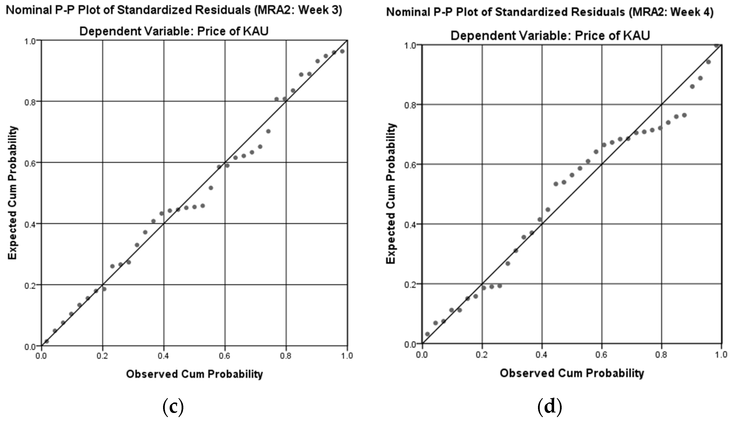
Figure 4 shows the normal P-P plot of regression standardized residual for testing the normality of the model estimation results for each time lag. Unlike the previous analysis, the model was analyzed only with statistically significant variables of each variable. Table 9 lists the variables used in the analysis model derived by time lag. Table 10, Table 11, Table 12 and Table 13 present the estimation results of the MRA model by time lag.

5.2. Timeseries Analysis Using ARIMA

5.2.1. Data Pre-Processing

This section explains the process of data pre-processing. R provides useful packages and functions in this matter, so it was used in this study. The ndiffs() function was used to deduce the number of differences required for a stationary series. The adf.test() function was used to conduct a unit root test. The acf() and pacf() functions were used to plot the ACF and PACF plots, respectively.
As mentioned in Step 4 of Figure 1, the trading price data were naturally converted to stabilize the variance to secure the time series normality of data for Timeseries Analysis. The number of differences in ARIMA analysis was determined as 1. Figure 5 presents the stabilized trading price data, and Table 14 lists the unit root test result of the trading price data.

5.2.2. Time Lag for an Appropriate Prediction Model

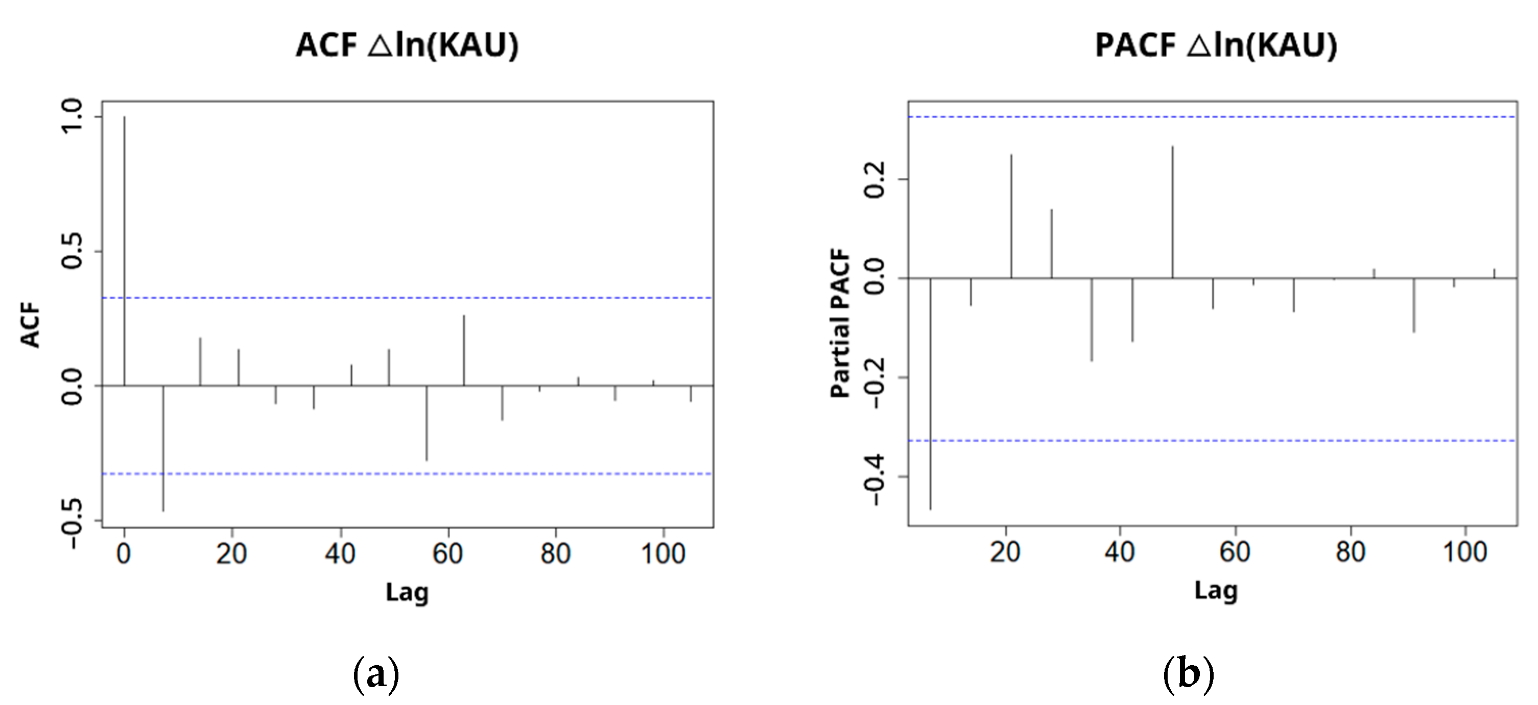
For the time lag selection of AR and MA, the model was estimated by considering the ACF (Auto Correlation Function) and PACF (Partial Auto Correlation Function) of the trading price data in Figure 6.
In ARIMA analysis, p , the time lag of AR, was used for analysis by reflecting the length of the time lag considered in the MRA and considering from 1 to 4. The time lag of MA, q , was fixed to 0. The time lag of d was analyzed by fixing it to 1 according to the number of differences in the previous unit root tests.

5.2.3. Model Derivation and Conformity Assessment

The suitability of the ARIMA(1,1,0), ARIMA(2,1,0), ARIMA(3,1,0), and ARIMA(4,1,0) models determined according to the previous process was diagnosed. The error satisfied the homogeneity of variance. There was no autocorrelation of the estimated model because there was no characteristic trend in the standardized residuals graph of Figure 7.
The time lag correlation through ACF statistics and Ljung–Box’s Q statistics confirms that white noise appears higher than the 5% significance level in most time lags. The null hypothesis of ‘time lag does not matter’ was satisfied [54].

6. Results

By comparing the adj-R2 representing the explanatory power of the derived MRA model, the prediction was attempted through the MRA model with the highest explanatory power for each analysis method, and the explanatory power of the MRA model for each time lag is shown in Table 15.
The predictions are attempted through the ARIMA model showing the lowest value by comparing the Akaike Information Criterion (AIC), which is an indicator for judging the appropriateness of the ARIMA model by the time lag. Table 16 lists the AIC for each ARIMA model [55].
The predictions are attempted through the four-week time lag MRA models of MRA1 and MRA2, which show the highest adj-R2 among the derived MRA models. Table 8 and Table 13 present the estimation results of each model. Table 17 lists the estimation results of the ARIMA(4,1,0) model showing the highest AIC value among the ARIMA models. Table 18 shows the results of actual trading price prediction through the ARIMA(4,1,0) model.
In this study, MAPE and MAE, with lower sensitivity to outliers and relatively higher reliability than the other predictions from evaluation indicators, were used to show the average error between the actual and predicted prices in the forecast period [52,54]. Equations (4) and (5) show the MAPE and MAE formula, respectively.
MAPE formula:
M A P E = 100 n t = 1 n | A c t u a l t P r e d i c t e d t A c t u a l t |    
MAE formula:
M A E = 1 n t = 1 n | A c t u a l t P r e d i c t e d t |
where A c t u a l t : actual value, P r e d i c t e d t : forecasted value, and n : number of samples
As a result of predicting the trading price after the next week of the analysis period, MAPE of 3.19 in the four-week time lag MRA model input, 2.75, and 0.113 in the ARIMA(4,1,0) model was shown, and the results of 847.31, 730.25, and 29.88 in the case of MAE.
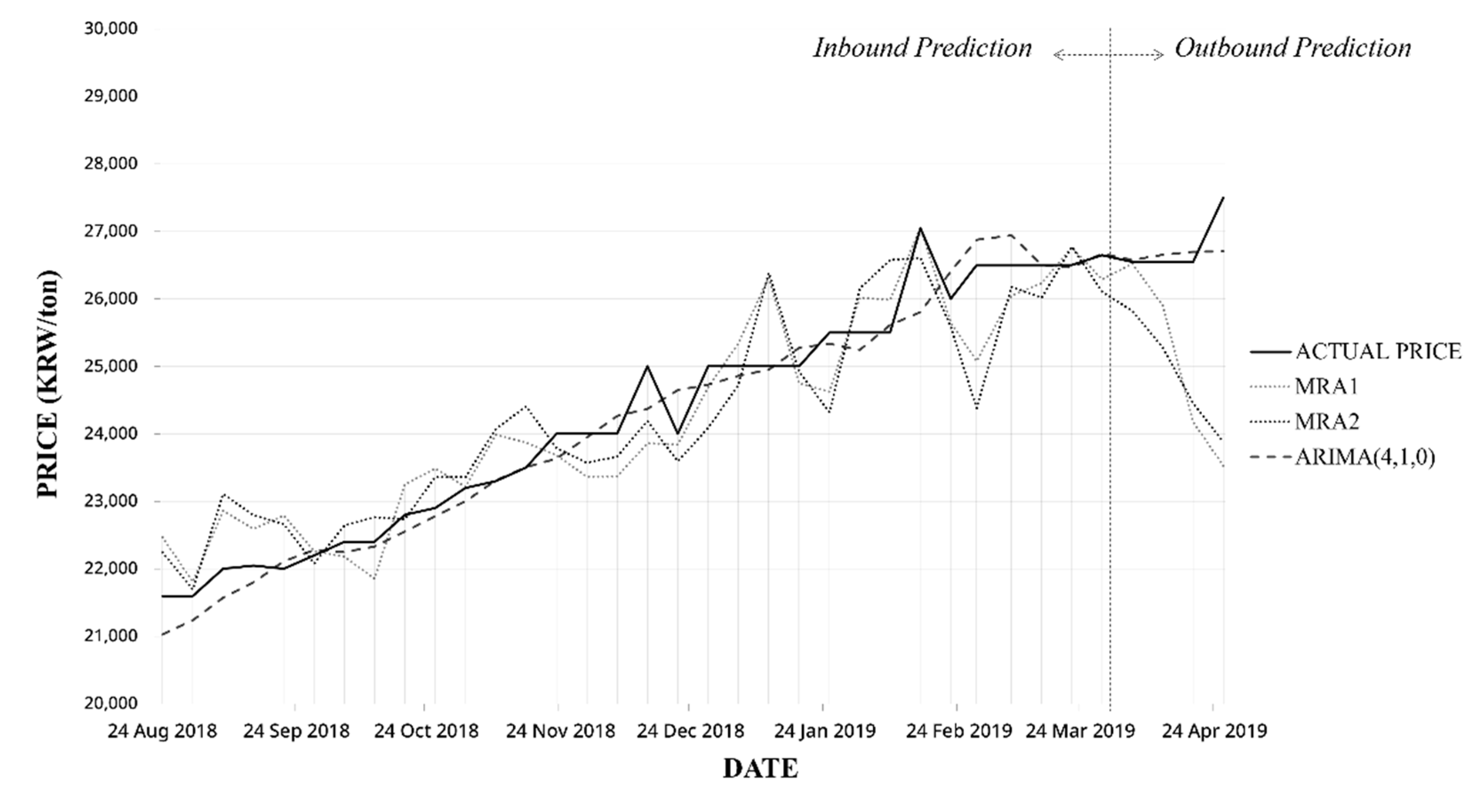
Table 19 lists the results of MAPE expressing the predictive power for the next four weeks of the analysis period by expanding the predictive period. The predictive power of the MRA model decreased with an increasing predictive period. Figure 8 shows a graph comparing the predicted trading price for each model and the value for the actual price. The prediction error of the MRA model increased with increasing analysis period. Table 20 lists the comparison results shown in Figure 8. As shown in Figure 8, the MRA1 and MRA2 models followed the same trend of actual price values in the inbound area. The MAPE and MAE for MRA1 and MRA2 were calculated based on Equations (4) and (5) and the values were calculated to be 2.11% MAPE for MRA1 and 2.39% MAPE for MRA2 in the inbound area. On the other hand, the MAPE and MAE increased dramatically in the outbound area (6.49% and 7.14%, respectively). This can also be seen in Figure 8, where MRA1 and MRA2 follow a declining trend in the outbound area. As for the ARIMA(4,1,0), the MAPE for the calculated inbound area was 1.07% and 0.99% in the outbound area. The ARIMA(4,1,0) showed great prediction results both in the inbound and outbound area, while MRA1 and MRA2 failed to predict the trend in the outbound area.

7. Discussion

This study derived an MRA prediction model and an ARIMA model using search query factors to reflect the behavior of market participants in predicting trading prices. The keywords extracted from papers related to emission rights and associated search terms derived from search engines were used, and trading prices corresponding to 37 weeks were applied.
The MRA model analysis results for each time lag confirmed that ‘themed stocks’ had a high correlation with the trading price when comparing the relative influence of search keyword keywords, including the med stocks related to carbon emissions, on trading price. In addition, significant search terms that can reflect the behavior of market participants related to trading prices were analyzed. Further research on the trading price prediction model focusing on the med stocks will be needed.
In the case of MRA, although it showed high predictive power to predict the trading price in the near future during the inbound analysis period, the error increased gradually at the outbound and followed a decreasing trend. The MRA confirmed that it is effective to update the analysis data and utilize the derived prediction model evenly. In the MRA model, the sudden rise and fall of the trading price were well reflected, but the error was larger than that of ARIMA, and the predictive power was relatively low for a long time. ARIMA, which reflects the behavior of the market participants, accurately reflected the long-term continuous rise in both inbound and outbound and showed the best results in the four-week prediction model.
Lamphiere et al. [33] produced ACF plots that showed distinct peaks at the medium and higher frequencies and indicated correlations within the data and memory effects at play. In the current study, however, there were no distinct peaks in the ACF plots. This difference was attributed to the dissimilarity in the analyzed data, where the data used in the current study show an increasing trend in general, unlike the work by Lamphiere et al. [33]. The maturity of the market plays a significant role in the matter of data variability and size.
Numerous studies on predicting and analyzing the correlations of carbon emission trading are being conducted worldwide. As mentioned in the literature review section, GARCH models have shown great potential in conducting such analysis [34,35,36,37,38]. Hence, they must be considered in future studies predicting and analyzing the correlations of KAU and different sources as different markets, environmental issues, and status in Korea.
In the case of ARIMA, the error was less than the credit prediction value using MRA, and the trend of the actual value was reflected. The results of the two models are derived differently in outbound because of the characteristics of the MRA and ARIMA models. MRA has high predictive power for the near future, but the error rate increases gradually with increasing analysis period, and ARIMA only differs in the degree of the upward trend but does not effectively represent price fluctuations and does not consider the influence of independent variables.

8. Conclusions

This study had significance in predicting the actual trading price in Korea, and the factors affecting the KAU were identified. For this purpose, the study conducted MRA and ARIMA. The independent variables used for regression were search queries connected to the largest search engine in Korea (Naver). As shown in Figure 8 and Table 20, the MAPE was quite promising for regression when predicting inbound values. Nevertheless, further studies need to assess other methodologies to achieve higher predictive accuracy at outbound values, while the ARIMA model showed good prediction results for both.
Attempts to predict the trading price and derived prediction models can help reduce the risk and uncertainty of the emission market to form a stable market. Policy help can be provided through the judgment of overheating and stagnation of the emission market. In addition, the prediction model of this study is expected to help investors make decisions at a time when the scope of the industry participating in ETS, the increase in the number of companies, and the expansion of participants, such as third-party market participation. On the industrial side, it is possible to check the purchase price and amount of emission rights using a model with a low error rate in process planning and the establishment and help calculate an accurate budget, considering environmental charges.
As a limitation, the predictive power through MRA was high, but the error rate increased gradually with increasing analysis period, and ARIMA showed high predictive power, but the price change was not effectively represented due to the characteristics of the model, and the effect of independent variables was not considered. Accordingly, the two models of this study require valid data. Future studies should consider the influence of independent variables, including the market participants’ behavior in the analysis and the prediction of the model, such as the MRA method and possibly different models, such as the GARCH model, as suggested in the discussion section. In addition, it is essential to study the analysis method with high predictive power and small errors simultaneously.

Author Contributions

Conceptualization, S.H.; methodology, H.K. and S.H.; software, H.K.; validation, H.K., Y.K. (Yujin Kim) and S.H.; formal analysis, H.K.; investigation, H.K.; resources, H.K.; data curation, H.K. and Y.K. (Yujin Kim); writing—original draft preparation, H.K. and Y.K. (Yujin Kim); writing—review and editing, Y.K. (Yujin Kim), Y.K. (Yongho Ko) and S.H.; visualization, Y.K. (Yujin Kim); supervision, S.H.; project administration, S.H.; revision and finalization, Y.K. (Yujin Kim), Y.K. (Yongho Ko) and S.H.; funding acquisition, S.H. All authors have read and agreed to the published version of the manuscript.

Funding

This research was supported by the National Research Foundation of Korea (NRF) grant funded by the Korean government (MSIT) (No. 2021R1A2C1007467).

Informed Consent Statement

Not applicable.

Data Availability Statement

Not applicable.

Conflicts of Interest

The authors declare no conflict of interest.

References

  1. Stern, N.; Stern, N.H. The Economics of Climate Change: The Stern Review; Cambridge University: Cambridge, UK, 2007. [Google Scholar]
  2. European Commission. EU ETS Handbook; European Commission: Brussels, Belgium, 2015; pp. 3–138. [Google Scholar]
  3. Beck, U.; Kruse-Andersen, P.K. Endogenizing the Cap in a Cap-and-Trade System: Assessing the Agreement on EU ETS Phase 4. Environ. Resour. Econ. 2020, 77, 781–811. [Google Scholar] [CrossRef]
  4. European Commission. Questions and Answers on the Provisional Agreement to Revise the EU Emissions Trading System (EU ETS); European Commission: Brussels, Belgium, 2017; pp. 1–4. [Google Scholar]
  5. Song, H.S. Activation of the 2050 Carbon Neutral and Emission Trading System; Issue Report 21–23; KCMI Korea Capital Market Institute: Seoul, Korea, 2021; pp. 1–21. [Google Scholar]
  6. European Commission. The Paris Protocol–A Blueprint for Tackling Global Climate Change Beyond; European Commission: Brussels, Belgium, 2020. [Google Scholar]
  7. Son, D.; Jeon, Y. Learning-by-doing Effect on Price Determination System in Korea’s Emission Trading Scheme. Environ. Resour. Econ. Rev. 2018, 27, 667–694. [Google Scholar]
  8. Lee, S.; Kim, D. Domestic Greenhouse Gas Emission Trading System Analysis of enforcement effects. Korean Environ. Inst. Res. Rep. 2017, 1–115. [Google Scholar]
  9. Son, I.; Kim, D.K. Analysis of the Impact of Key Design Elements for the EU-ETS Phase 4 on the K-ETS in the Future. Environ. Resour. Econ. Rev. 2021, 30, 129–167. [Google Scholar]
  10. Yoo, I. Domestic Emission Trading Market Issues and Prospects for 2021. KONETIC, 2021; pp. 2–9. Available online: https://www.konetic.or.kr/user/P/PA/PA001_L01.do (accessed on 1 September 2021).
  11. K-eco (Korea Environment Corporation). GHG Reduction Policy Support. Available online: https://www.keco.or.kr/kr/business/climate/contentsid/1520/index.do (accessed on 1 February 2022).
  12. Lee, J.Y.; Seol, G.; Yoon, N.R.; Lee, M.K.; Lee, S.W.; Lee, S.Y.; Lee, J.H.; Jeong, Y.M. 2018 K-ETS Summary Report; President of the Greenhouse Gas Inventory and Research Center of Korea: Seoul, Korea, 2020; pp. 1–40. [Google Scholar]
  13. Benz, E.; Trück, S. Modeling the price dynamics of CO2 emission allowances. Energy Econ. 2009, 31, 4–15. [Google Scholar] [CrossRef]
  14. Chevallier, J. Carbon futures and macroeconomic risk factors: A view from the EU ETS. Energy Econ. 2009, 31, 614–625. [Google Scholar] [CrossRef]
  15. Zhu, B.; Chevallier, J. Carbon Price Forecasting with a Hybrid ARIMA and Least Squares Support Vector Machines Methodology. In Pricing and Forecasting Carbon Markets; Springer: Cham, Switzerland, 2017; pp. 87–107. [Google Scholar] [CrossRef]
  16. Sun, W.; Huang, C. A carbon price prediction model based on secondary decomposition algorithm and optimized back propagation neural network. J. Clean. Prod. 2020, 243, 118671. [Google Scholar] [CrossRef]
  17. Koop, G.; Tole, L. Forecasting the European carbon market. J. R. Stat. Soc. Ser. A 2013, 176, 723–741. [Google Scholar] [CrossRef] [Green Version]
  18. Zhang, J.; Li, D.; Hao, Y.; Tan, Z. A hybrid model using signal processing technology, econometric models and neural network for carbon spot price forecasting. J. Clean. Prod. 2018, 204, 958–964. [Google Scholar] [CrossRef]
  19. Ministry of Environment. 3rd Basic Plan for Emission Transaction System. 2019, pp. 1–35. Available online: https://www.gihoo.or.kr/portal/kr/community/data_view.do?p=1&idx=20483&column=&groupname=data&groupid=&f=1&q (accessed on 1 April 2020).
  20. Çanakoğlu, E.; Adıyeke, E.; Ağralı, S. Modeling of carbon credit prices using regime switching approach. J. Renew. Sustain. Energy 2018, 10, 035901. [Google Scholar] [CrossRef]
  21. Kim, Y.; Ahn, J. The Study on Development of Carbon Emission Price Forecasting Model Reflecting Emission Trading Market Characteristics. Entrue J. Inf. Technol. 2016, 15, 7–16. [Google Scholar]
  22. Kim, S. Analysis and Prospects of Price Determinants of Emissions Trading; Korea Energy Economics Institute: Seoul, Korea, 2007. [Google Scholar]
  23. Chevallier, J. EUAs and CERs: Vector autoregression, impulse response function and cointegration analysis. Econ. Bull. 2010, 30, 558–576. [Google Scholar]
  24. Chevallier, J. Nonparametric modeling of carbon prices. Energy Econ. 2011, 33, 1267–1282. [Google Scholar] [CrossRef]
  25. Conrad, C.; Rittler, D.; Rotfuß, W. Modeling and explaining the dynamics of European Union Allowance prices at high-frequency. Energy Econ. 2012, 34, 316–326. [Google Scholar] [CrossRef] [Green Version]
  26. Guðbrandsdóttir, H.N.; Haraldsson, H. Predicting the Price of EU ETS Carbon Credits. Syst. Eng. Procedia 2011, 1, 481–489. [Google Scholar] [CrossRef] [Green Version]
  27. Chevallier, J. Carbon price drivers: An updated literature review. Int. J. Appl. Logist. 2013, 4, 1–7. [Google Scholar] [CrossRef] [Green Version]
  28. Reboredo, J.C. Modeling EU allowances and oil market interdependence. Implications for portfolio management. Energy Econ. 2013, 36, 471–480. [Google Scholar] [CrossRef]
  29. Yahşi, M.; Çanakoğlu, E.; Ağralı, S. Carbon price forecasting models based on big data analytics. Carbon Manag. 2019, 10, 175–187. [Google Scholar] [CrossRef]
  30. Zhao, X.; Han, M.; Ding, L.; Kang, W. Usefulness of economic and energy data at different frequencies for carbon price forecasting in the EU ETS. Appl. Energy 2018, 216, 132–141. [Google Scholar] [CrossRef]
  31. Hao, Y.; Tian, C.; Wu, C. Modelling of carbon price in two real carbon trading markets. J. Clean. Prod. 2020, 244, 118556. [Google Scholar] [CrossRef]
  32. Kim, H.; Im, G.; Kim, Y.; Lee, M.; Han, S. The Comparison of Certified Emission Reductions Forecasting Model Using Price of Certified Emission Reductions and Related Search Keywords. In Proceedings of the Korean Institute of Building Construction Conference 2020, Seoul, Korea, 12 June 2020; pp. 44–45. [Google Scholar]
  33. Lamphiere, M.; Blackledge, J.; Kearney, D. Carbon Futures Trading and Short-Term Price Prediction: An Analysis Using the Fractal Market Hypothesis and Evolutionary Computing. Mathematics 2021, 9, 1005. [Google Scholar] [CrossRef]
  34. Zhang, Y.-J.; Sun, Y.-F. The dynamic volatility spillover between European carbon trading market and fossil energy market. J. Clean. Prod. 2016, 112, 2654–2663. [Google Scholar] [CrossRef]
  35. Wei, L.; Can, L. The research on setting a unified interval of carbon price benchmark in the national carbon trading market of China. Appl. Energy 2015, 155, 728–739. [Google Scholar]
  36. Zhibin, L.; Shan, H. Carbon option price forecasting based on modified fractional Brownian motion optimized by GARCH model in carbon emission trading. North Am. J. Econ. Financ. 2021, 55, 101307. [Google Scholar]
  37. Loperfido, N. Kurtosis-based projection pursuit for outlier detection in financial time series. Eur. J. Financ. 2019, 26, 142–164. [Google Scholar] [CrossRef]
  38. Yun, P.; Zhang, C.; Wu, Y.; Yang, Y. Forecasting Carbon Dioxide Price Using a Time-Varying High-Order Moment Hybrid Model of NAGARCHSK and Gated Recurrent Unit Network. Int. J. Environ. Res. Public Health 2022, 19, 899. [Google Scholar] [CrossRef] [PubMed]
  39. Ginsberg, J.; Mohebbi, M.H.; Patel, R.S.; Brammer, L.; Smolinski, M.S.; Brilliant, L. Detecting influenza epidemics using search engine query data. Nature 2009, 457, 1012–1014. [Google Scholar] [CrossRef]
  40. Da, Z.; Engelberg, J.; Gao, P. In search of attention. J. Financ. 2011, 66, 1461–1499. [Google Scholar] [CrossRef]
  41. Joseph, K.; Wintoki, M.B.; Zhang, Z. Forecasting abnormal stock returns and trading volume using investor sentiment: Evidence from online search. Int. J. Forecast. 2011, 27, 1116–1127. [Google Scholar] [CrossRef]
  42. Han, S.; Ko, Y.; Kim, J.-Y.; Shin, D.H. Enhancement of Prediction Accuracy for Home Sales Index Prediction Model based on Integration of Multiple Regression Analysis and Genetic Algorithm. KSCE J. Civ. Eng. 2018, 22, 2159–2166. [Google Scholar] [CrossRef]
  43. Beracha, E.; Wintoki, M.B. Forecasting Residential Real Estate Price Changes from Online Search Activity. J. Real Estate Res. 2013, 35, 283–312. [Google Scholar] [CrossRef]
  44. Goel, S.; Hofman, J.M.; Lahaie, S.; Pennock, D.M.; Watts, D.J. Predicting consumer behavior with Web search. Proc. Natl. Acad. Sci. USA 2010, 107, 17486–17490. [Google Scholar] [CrossRef] [PubMed] [Green Version]
  45. BizSpring Inc. Statistics. Available online: http://www.internettrend.co.kr/trendForward.tsp (accessed on 1 July 2019).
  46. Naver. Search Term Trend. Available online: http://datalab.naver.com/keyword/trendSearch.naver (accessed on 4 March 2022).
  47. Neter, J.; Kutner, M.H.; Nachtsheim, C.J.; Wasserman, W. Applied Linear Statistical Models; Irwin: Chicago, IL, USA, 1996. [Google Scholar]
  48. Nam, J.-O.; Noh, S.-G. A Study on Forecast of Oyster Production using Time Series Models. Ocean Polar Res. 2012, 34, 185–195. [Google Scholar] [CrossRef] [Green Version]
  49. Hyndman, R.J.; Athanasopoulos, G. Forecasting: Principles and Practice, 3rd ed.; OTexts: Melbourne, Australia, 2018. [Google Scholar]
  50. Han, S.; Ko, Y.; Kim, J.; Hong, T. Housing Market Trend Forecasts through Statistical Comparisons based on Big Data Analytic Methods. J. Manag. Eng. 2018, 34, 04017054. [Google Scholar] [CrossRef]
  51. Devore, J. Probability and Statistics for Engineering and Science, 8th ed.; Richard Stratton: New York, NY, USA, 2012; pp. 1–712. [Google Scholar]
  52. Ryu, N.; Kim, H.; Kang, P. Evaluating Variable Selection Techniques for Multivariate Linear Regression. J. Korean Inst. Ind. Eng. 2016, 42, 314–326. [Google Scholar] [CrossRef] [Green Version]
  53. Asuero, A.G.; Sayago, A.; Gonzalez, A.G. The Correlation Coefficient: An Overview. Crit. Rev. Anal. Chem. 2006, 36, 41–59. [Google Scholar] [CrossRef]
  54. Im, C.Y.; Kim, H.C. A Study on the Analysis and Prediction of Housing Mortgage in Deposit Bank Using ARIMA Model. J. Korea Inst. Inf. Electron. Commun. Technol. 2019, 12, 265–272. [Google Scholar]
  55. Min, K.-C.; Jun, Y.-I.; Ha, H.-K. Forecasting the Air Cargo Demand with Seasonal ARIMA Model: Focusing on ICN to EU Route. J. Korean Soc. Transp. 2013, 31, 3–18. [Google Scholar] [CrossRef]
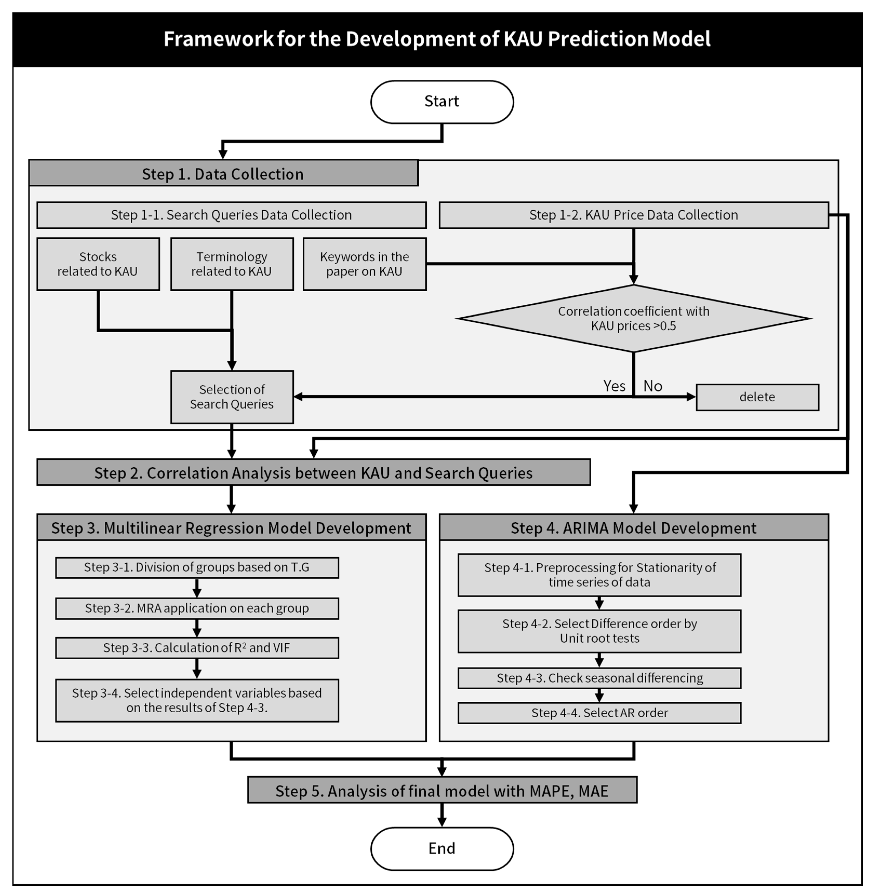
Figure 1. Framework for the development of the KAU prediction model (own creation).
Sustainability 14 08177 g001
Figure 2. KAU trend (source: https://ets.krx.co.kr).
Sustainability 14 08177 g002
Figure 4. Nominal P-P plot of regression standardized residential of MRA2 (own creation): (a) One-week time lag MRA model with statistically significant variables; (b) two-week time lag MRA model with statistically significant variables; (c) three-week time lag MRA model with statistically significant variables; (d) four-week time lag MRA model with statistically significant variables.
Sustainability 14 08177 g004aSustainability 14 08177 g004b
Figure 5. Stabilized KAU data (own creation).
Sustainability 14 08177 g005
Figure 6. ACF and PACF of the KAU data (own creation): (a) Autocorrelation function of Korean Allowance Unit; (b) Partial autocorrelation function of Korean Allowance Unit.
Sustainability 14 08177 g006
Figure 7. Conformity diagnosis of ARIMA model (own creation): (a) Standardized residuals graph, ACF of residuals graph, significance probability graph of ARIMA(1,1,0); (b) standardized residuals graph, ACF of residuals graph, significance probability graph of ARIMA(2,1,0); (c) standardized residuals graph, ACF of residuals graph, significance probability graph of ARIMA(3,1,0); (d) standardized residuals graph, ACF of residuals graph, significance probability graph of ARIMA(4,1,0).
Sustainability 14 08177 g007
Figure 8. Graph of the actual price and predicted price by prediction models (own creation).
Sustainability 14 08177 g008
Table 1. Search queries basic statistics.
KeywordsMeanS.DMinimumMedianMaximumSize
CET *108.741.038.5109.1198.937
FOOSUNG23,663.77092.711,293.822,554.545,426.437
CETS **369.2155.2120.4360.2733.437
EAGON11,542.58320.63555.19609.542,022.237
Price of CERs54.044.50.043.8213.637
HH ***11,809.85206.75330.910,853.027,770.437
UNISON16,969.44586.87856.316,120.134,258.337
HOMEDECO1176.7218.6863.21155.31935.637
HUCHEMS4862.71144.52336.94692.97703.037
productive1675.0520.4973.71470.62869.637
productivity1425.9342.9798.21370.52507.437
compare1820.6436.71285.71771.33289.337
excavator855.680.4709.1861.11083.337
emissions766.4194.6445.2750.61201.037
CO2 emissions14.013.50.09.655.737
GW ****280.153.5155.4287.7370.537
NOx4087.3755.73007.93991.26967.737
PEMS168.9163.10.0122.3914.037
durable2100.4475.31150.92075.83443.737
furniture3026.7536.91906.22902.24546.037
wakefulness83.751.212.670.7222.137
S.D: Standard Deviation; * CET: Carbon Emission Trading; ** CETS: Carbon Emission Trading System; *** HH: Hansol Homedeco; **** GW: Global Warming. (source: http://datalab.naver.com/keyword/trendSearch.naver).
Table 2. KAU data basic statistics (source: https://ets.krx.co.kr).
DataMeanStandard DeviationMinimumMedianMaximumSize
KAU23,931.0811770.13621,60024,00027,05037
Table 3. Correlation coefficient by parallax of search queries data (own creation).
VariableWeek 1Week 2Week 3Week 4
CET *−0.149−0.211−0.247−0.363
FOOSUNG−0.39−0.417−0.493−0.532
CETS **−0.317−0.316−0.341−0.384
EAGON−0.368−0.346−0.359−0.374
Price of CER−0.313−0.356−0.465−0.507
HANSOLHOMEDECO−0.469−0.419−0.433−0.456
UNISON−0.191−0.146−0.213−0.223
HOMEDECO0.5780.6230.6660.702
HUCHEMS0.1660.1830.0660.075
productive0.6560.6710.6630.635
productivity0.3990.4580.470.462
Compare0.5360.5030.4590.464
Excavator−0.444−0.218−0.215−0.319
emissions0.4680.5370.5290.548
CO2 emissions0.140.1120.097−0.022
global warming−0.161−0.101−0.0670.02
NOx−0.080.0250.1020.168
PEMS−0.089−0.017−0.037−0.02
durable0.5130.4990.4640.387
furniture0.2850.3140.3340.348
wakefulness0.5820.5430.50.482
* CET: Carbon Emission Trading; ** CETS: Carbon Emission Trading System.
Table 4. Variable used by MRA 1 (own creation).
Time GapSearch Queries
Week 1HOMEDECO, productive, compare, durable, wakefulness
Week 2HOMEDECO, productive, compare, emissions, wakefulness
Week 3HOMEDECO, productive, emissions, wakefulness
Week 4FOOSUNG, price of CER, HOMEDECO, productive, emissions
Table 5. Time lag: Week 1, MRA1 estimation results (own creation).
VariableCoefficientS.EtPrVIFadj-R2D.W.
US
HOMEDECO2.9340.3630.7284.0280.0001.1250.7401.395
productive2.1130.6220.4185.0570.0002.092
compare1.9600.4750.6453.0360.0053.386
durable−1.693−0.4530.688−2.4610.0204.687
wakefulness8.2560.2333.8922.1210.0421.671
(Constant)16,306.254-1062.46515.3480.000-
U: Unstandardized; S: Standardized; S.E: Standard Error; Pr: Probability; VIF: Variance Inflation Factor adj-R2: adjusted R2; D.W.: Durbin Watson.
Table 6. Time lag: Week 2, MRA1 estimation results (own creation).
VariableCoefficientS.EtPrVIFadj-R2D.W.
US
HOMEDECO3.5050.4350.8324.2110.0001.2710.6981.281
productive1.5450.4550.3804.064 0.000 1.491
emissions−0.035−0.0041.074−0.033 0.974 1.665
compare0.8210.1840.4911.6720.105 1.446
wakefulness5.2590.1354.4121.192 0.242 1.522
(Constant)15,428.686-1124.78213.7170.000 -
U: Unstandardized; S: Standardized; S.E: Standard Error; Pr: Probability; VIF: Variance Inflation Factor. adj-R2: adjusted R2; D.W.: Durbin Watson.
Table 7. Time lag: Week 3, MRA1 estimation results (own creation).
VariableCoefficientS.EtPrVIFadj-R2D.W.
US
HOMEDECO3.958 0.4920.8544.635 0.000 1.3060.698 1.281
productive1.658 0.4890.381 4.3500.000 1.465
emissions0.138 0.0151.075 0.129 0.898 1.620
wakefulness5.254 0.1284.362 1.205 0.237 1.310
(Constant)16,093.189-980.468 16.4140.000-
U: Unstandardized; S: Standardized; S.E: Standard Error; Pr: Probability; VIF: Variance Inflation Factor. adj-R2: adjusted R2; D.W.: Durbin Watson.
Table 8. Time lag: Week 4, MRA1 estimation results (own creation).
VariableCoefficientS.EtPrVIFadj-R2D.W.
US
HOMEDECO2.415 0.3024.068 −0.797 0.434 2.322 0.822 1.561
productive1.758 0.5080.030 −2.867 0.009 4.460
emissions1.210 0.1331.756 −0.298 0.769 6.302
FOOSUNG−0.085 −0.4080.018 1.150 0.261 1.963
price of CER−1.4410.0434.353 0.194 0.848 3.613
(Constant)19,590.524-1098.55317.8330.000 -
U: Unstandardized; S: Standardized; S.E: Standard Error; Pr: Probability; VIF: Variance Inflation Factor. adj-R2: adjusted R 2 ; D.W.: Durbin Watson.
Table 9. Variable used by MRA2 (own creation).
Time GapSearch Queries
Week 1productive, HOMEDECO, wakefulness
Week 2productive, HOMEDECO, compare
Week 3HOMDECO, productive
Week 4HOMEDECO, productive, FOOSUNG
Table 10. Time lag: Week 1, MRA2 model estimation results (own creation).
VariableCoefficientS.EtPrVIF adj - R 2 D.W.
US
productive1.5620.4600.3444.5430.0001.1580.6821.262
HOMEDECO3.0980.3840.8003.8740.0001.109
wakefulness11.2640.3183.6313.1020.0041.189
(Constant)16,774.013-972.62117.2460.000-
U: Unstandardized; S: Standardized; S.E: Standard Error; Pr: Probability; VIF: Variance Inflation Factor. adj- R 2 : adjusted R 2 ; D.W.: Durbin Watson.
Table 11. Time lag: Week 2, MRA2 model estimation results (own creation).
VariableCoefficientS.EtPrVIF adj - R 2 D.W.
US
HOMEDECO2.6580.3330.6893.8610.0001.4990.7031.281
productive2.0300.5870.2647.6960.0001.174
FOOSUNG−0.090−0.4340.017−5.2110.0001.398
(Constant)19,825.066-1023.65219.3670.000 -
U: Unstandardized; S: Standardized; S.E: Standard Error; Pr: Probability; VIF: Variance Inflation Factor. adj- R 2 : adjusted R 2 ; D.W.: Durbin Watson.
Table 12. Time lag: Week 3, MRA2 model estimation results (own creation).
VariableCoefficientS.EtPrVIF adj - R 2 D.W
US
HOMEDECO4.3180.5370.7655.6430.000 1.063 0.6941.064
productive1.806 0.5330.322 5.602 0.000 1.063
(Constant)15,901.400 -938.182 16.949 0.000 -
U: Unstandardized; S: Standardized; S.E: Standard Error; Pr: Probability; VIF: Variance Inflation Factor. adj- R 2 : adjusted R 2 ; D.W.: Durbin Watson.
Table 13. Time lag: Week 4, MRA2 model estimation results (own creation).
VariableCoefficientS.EtPrVIF adj - R 2 D.W
US
HOMEDECO2.6580.3330.6893.8610.0001.4990.8221.608
productive2.0300.5870.2647.6960.0001.174
FOOSUNG−0.090−0.4340.017−5.2110.0001.398
(Constant)19,825.066 -1023.65219.3670.000-
U: Unstandardized; S: Standardized; S.E: Standard Error; Pr: Probability; VIF: Variance Inflation Factor. adj- R 2 : adjusted R 2 ; D.W.: Durbin Watson.
Table 14. Augmented Dickey–Fuller (ADF) test result of KAU data (own creation).
Dependent VariableVariableFirst Difference
t-StatisticPrt-StatisticPr
KAU–2.91670.2158–3.84590.02834
Pr: Probability.
Table 15. Adj-R2 by the MRA Models (own creation).
ModelWeek 1Week 2Week 3Week 4
MRA 10.7400.6980.6890.822
MRA 20.6820.7030.6940.822
Table 16. AIC (Akaike information criterion) of ARIMA models (own creation).
ModelARIMA(1,1,0)ARIMA(2,1,0)ARIMA(3,1,0)ARIMA(4,1,0)
AIC−183.93−182.11−183.2−184.09
Table 17. ARIMA(4,1,0) model estimated results (own creation).
VariableCoefficientStandard ErrorzPr
(Constant)0.00070.00630.11440.9089
AR(1)−0.51920.1560−3.32690.0008
AR(2)0.20800.17311.20180.2294
AR(3)0.58240.18573.13580.0017
AR(4)0.31910.17251.84980.0643
AIC−184.09
Log-likelihood98.05
Pr: Probability.
Table 18. Result of each model’s prediction at 2019.04.05 (Outbound 1 Week) (own creation).
Dependent VariableMRATime Series
Time Lag: Week 4
(MRA1)
Time Lag: Week 4
(MRA2)
ARIMA(4,1,0)
Predicted Price
(KRW/ton)
25,702.6925,819.7526,579.88
Actual Price
(KRW/ton)
26,55026,55026,550
MAPE3.192.750.11
MAE847.31730.2529.88
Table 19. Forecasts for the next four weeks (Outbound weeks 1–4) (own creation).
Time Lag: Week 4 (MRA1)Time Lag: Week 4 (MRA2)ARIMA(4,1,0)
MAPE7.317.140.99
Table 20. Quantified comparison of the prediction models (own creation).
InboundOutbound
MRA1MRA2ARIMA(4,1,0)MRA1MRA2ARIMA(4,1,0)
MAPE2.112.391.076.497.140.99
MAE509.37583.89261.271756.251927.99269.07
Publisher’s Note: MDPI stays neutral with regard to jurisdictional claims in published maps and institutional affiliations.