Vehicle Recognition from Unmanned Aerial Vehicle Videos Based on Fusion of Target Pre-Detection and Deep Learning

Abstract

For accurate and effective automatic vehicle identification, morphological detection and deep convolutional networks were combined to propose a method for locating and identifying vehicle models from unmanned aerial vehicle (UAV) videos. First, the region of interest of the video frame image was sketched and grey-scale processing was performed; sub-pixel-level skeleton images were generated based on the Canny edge detection results of the region of interest; then, the image skeletons were decomposed and reconstructed. Second, a combination of morphological operations and connected domain morphological features were applied for vehicle target recognition, and a deep learning image benchmark library containing 244,520 UAV video vehicle samples was constructed. Third, we improved the AlexNet model by adding convolutional layers, pooling layers, and adjusting network parameters, which we named AlexNet*. Finally, a vehicle recognition method was established based on a candidate target extraction algorithm with AlexNet*. The validation analysis revealed that AlexNet* achieved a mean $F_1$ of 85.51% for image classification, outperforming AlexNet (82.54%), LeNet (63.88%), CaffeNet (46.64%), VGG16 (16.67%), and GoogLeNet (14.38%). The mean values of $P_{cor}$, $P_{re}$, and $P_{miss}$ for cars and buses reached 94.63%, 6.87%, and 4.40%, respectively, proving that this method can effectively identify UAV video targets.

1. Introduction

Recently, traffic congestion has become a major problem in large cities and even small- and medium-sized cities in China and abroad. Effective monitoring and control of urban traffic have become urgent for transportation departments and the general public in all countries. To ensure the efficient operation of traffic and to meet the travel needs of the public, one of the important prerequisites and key conditions lies in real-time, efficient access to traffic information. Accordingly, many cities have deployed fixed-type detectors such as induction coils, fixed-point cameras, and RFID to obtain cross-sectional traffic information, and use mobile devices such as floating vehicles to extract dynamic traffic information based on GPS, providing a large amount of basic data for urban traffic operation.

With the increasing requirements of urban traffic supervision, video image detection technology has rapidly developed, and the popularity of drones in the civilian sector had gradually increased. Since 2002, the United States, Germany, Korea, and China have been exploring the utilization of drones to observe the traffic status in urban wide-area scenarios [1,2,3,4]. Comparing modern urban traffic systems with ground-based traffic information detection equipment, UAVs equipped with video inspection platforms have a variety of advantages such as being lightweight and low cost, and having easy handling, wide monitoring range, and no effects on road traffic. They are suitable for traffic monitoring in urban arterial areas, key road sections and nodes, and other important parts of the road network, and can be used as an effective supplement to the existing traffic information detection methods.

The basis and key of UAV traffic information acquisition depend on video vehicle detection, which has attracted keen attention from researchers. Scholars found that the accuracy of the information collected by the UAV was highly dependent on the stabilization of the video and the georeferencing procedure [5]. Vehicle detection is mostly performed by designing algorithms to extract image features [6,7]. However, due to the complexity of the traffic scene, the relevant feature extraction process is tedious and more sensitive to changes in vehicle scale, and the detection effect often fails to meet expectations when the target objects are relatively small and the distance between the target objects is very close. As a result, some scholars have proposed multi-scale target detection algorithms to solve the problem of multi-scale vehicle detection under large-sized aerial images [8]. The response time required for moving target objects in video tracking is reduced by methods such as video inter-frame motion estimation and dynamic computational offloading schemes [9,10]. Additionally, it tries to prevent the possibility of the algorithm updating the assignment indefinitely without completing all vehicle checks, which promotes the development of video traffic information collection effectively [11].

Since the detection efficiency and robustness of video image vehicle recognition in complex environments are still poor, deep learning is gradually emerging in large-scale image classification and localization. Some scholars have focused on video target recognition based on deep neural networks. Alex Krizhevsky’s team proposed the famous AlexNet model based on deep convolutional neural networks (CNN), which became a landmark advance in deep learning in the field of large-scale image classification [12]. Then, deep convolutional neural networks, such as the convolutional architecture for fast feature-embedding networks (CaffeNet), visual geometry group 16 layers (VGG16), and GoogLeNet, have been proposed [13]. Many scholars have also started to conduct vehicle-detection-related research using deep learning models, applying CNN and support vector machine (SVM) methods for vehicle identification in UAV images [14]. Some scholars applied CNN and a hard-case-mining-based vehicle detection method for satellite images and an improved faster regions with CNN features (R-CNN) method for traffic scene vehicle detection by applying MIT and Caltech vehicle datasets [15,16]. These studies proposed deep learning models based on CNN, Faster R-CNN, and other deep learning models for cell phones, vehicles, license plates, pedestrian, and traffic sign detection methods; although, there are relatively few studies on vehicle detection specifically for UAV videos. Compared with traditional image detection methods, deep convolutional neural networks can simulate human brain neural networks for data hierarchical description, which can usually obtain a large number of multi-scale image features, whose recognition results are usually closer to the actual situation, with higher accuracy and effective image classification.

In summary, the complex and variable urban traffic video scenes from UAVs often make it difficult to manually extract reasonable features to effectively identify vehicle targets. To effectively combine the advantages of traditional image detection with deep learning to recognize vehicle targets accurately, we proposed a UAV video vehicle localization and model recognition method based on morphological detection fused with the AlexNet deep convolutional network, and we constructed a dataset for testing and analysis. The proposed detection framework consists of the following four steps:

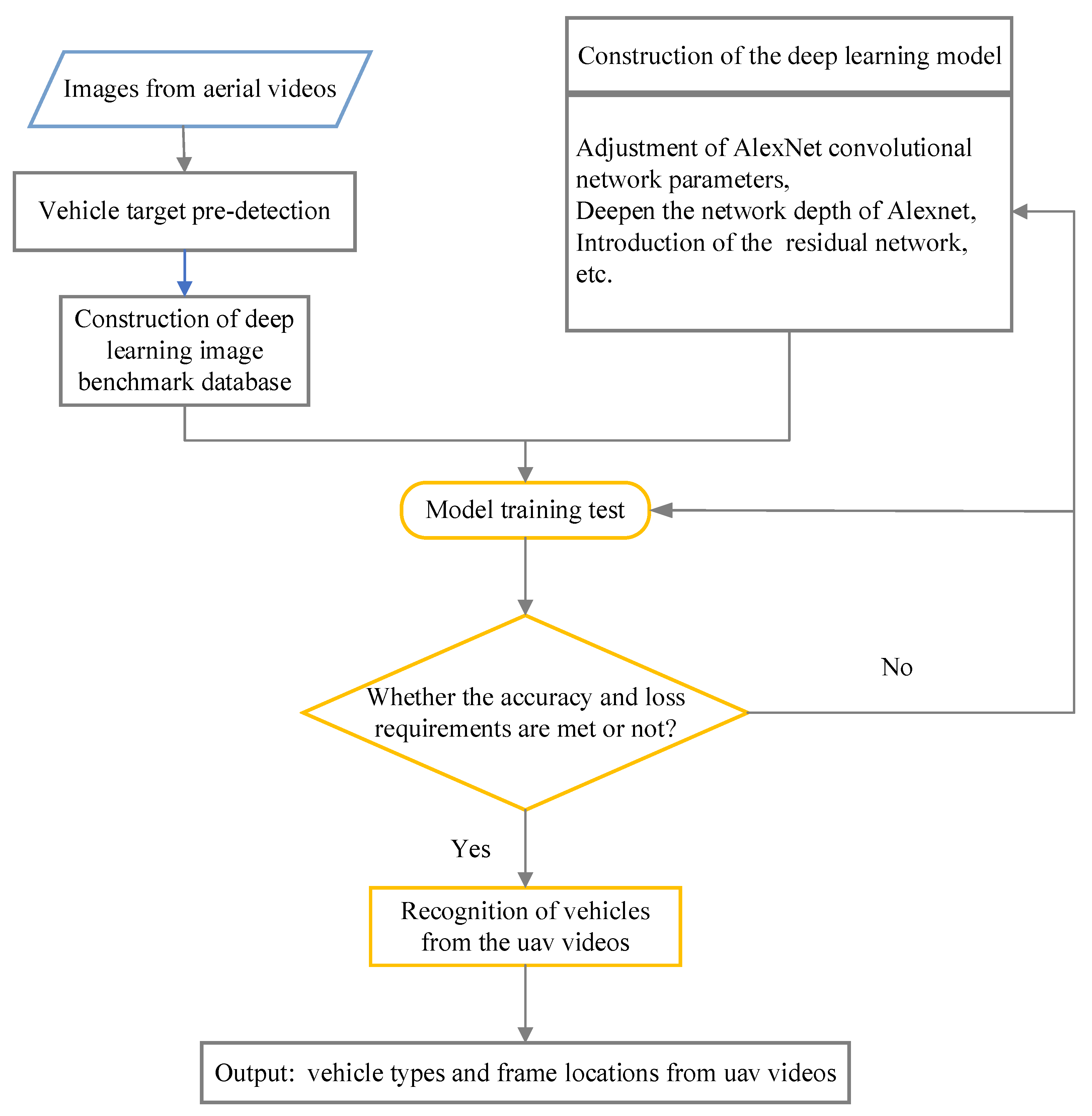
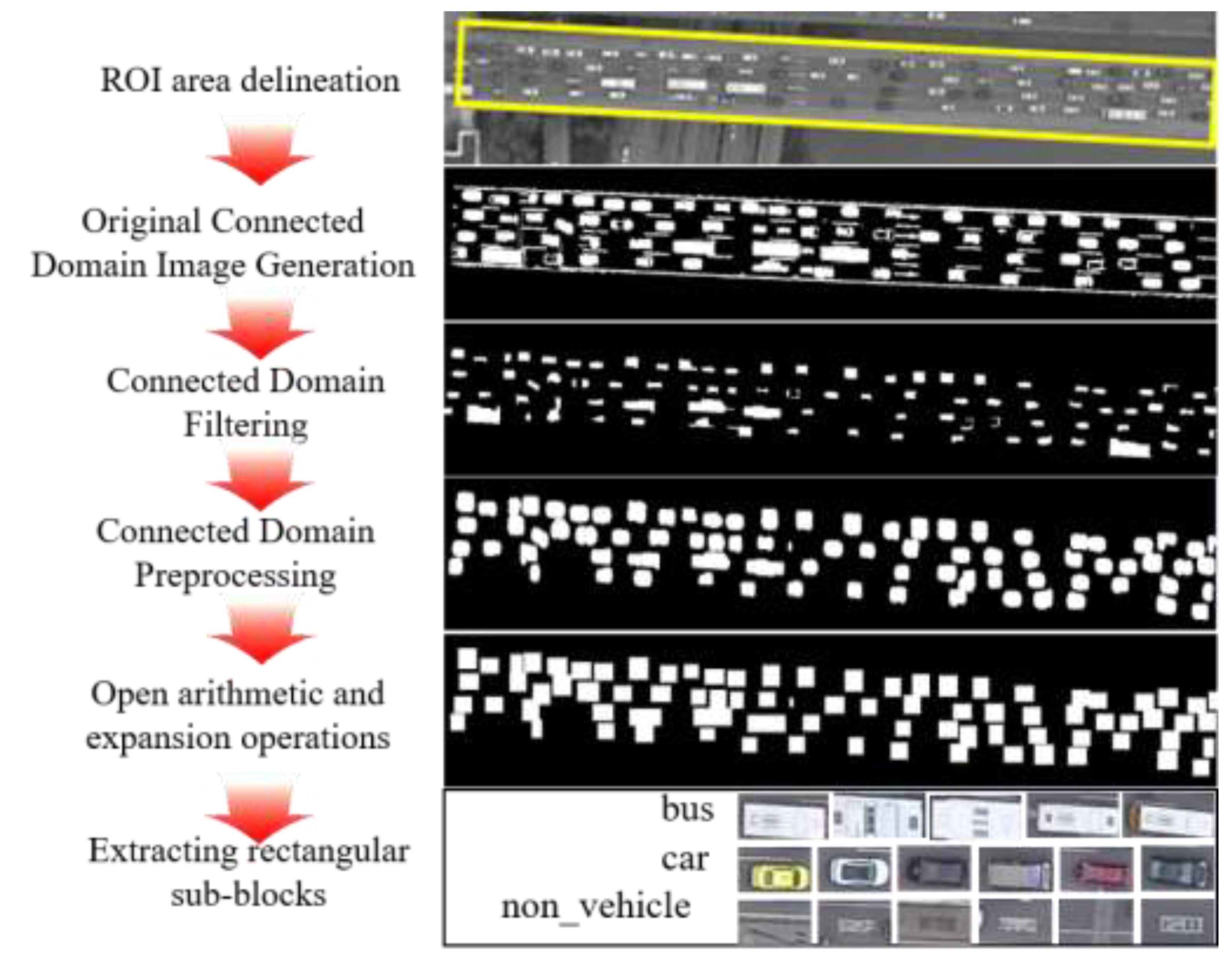
• UAV high-resolution video vehicles target pre-detection: we used techniques including edge detection, morphology analysis, image skeleton structure reconstruction, and connected domain feature analysis to identify the connected domains that satisfy the preset conditions. The connected domains were used as candidate vehicle target regions.
• Image benchmark library construction: the candidate vehicle target areas were taken and sorted manually. The image benchmark library was constructed containing training image sets, test image sets, and validation image sets of bus, car, and non-vehicle. Non-vehicle in the present paper includes lane lines, trees, railings, other traffic signs, etc.
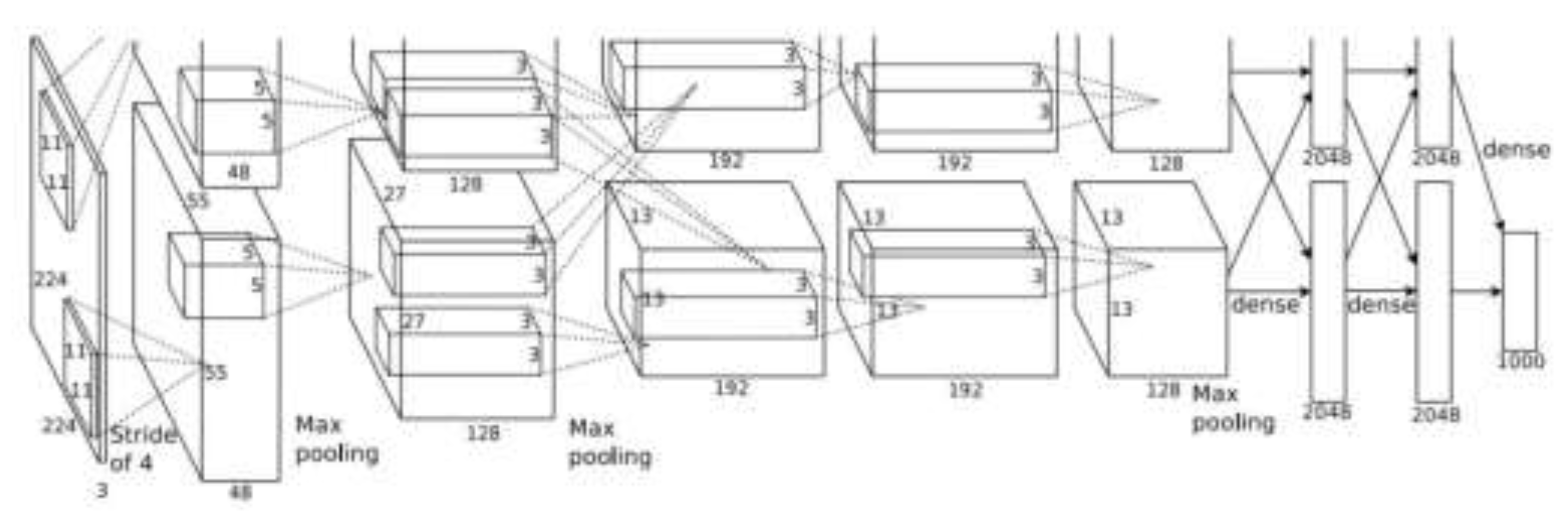
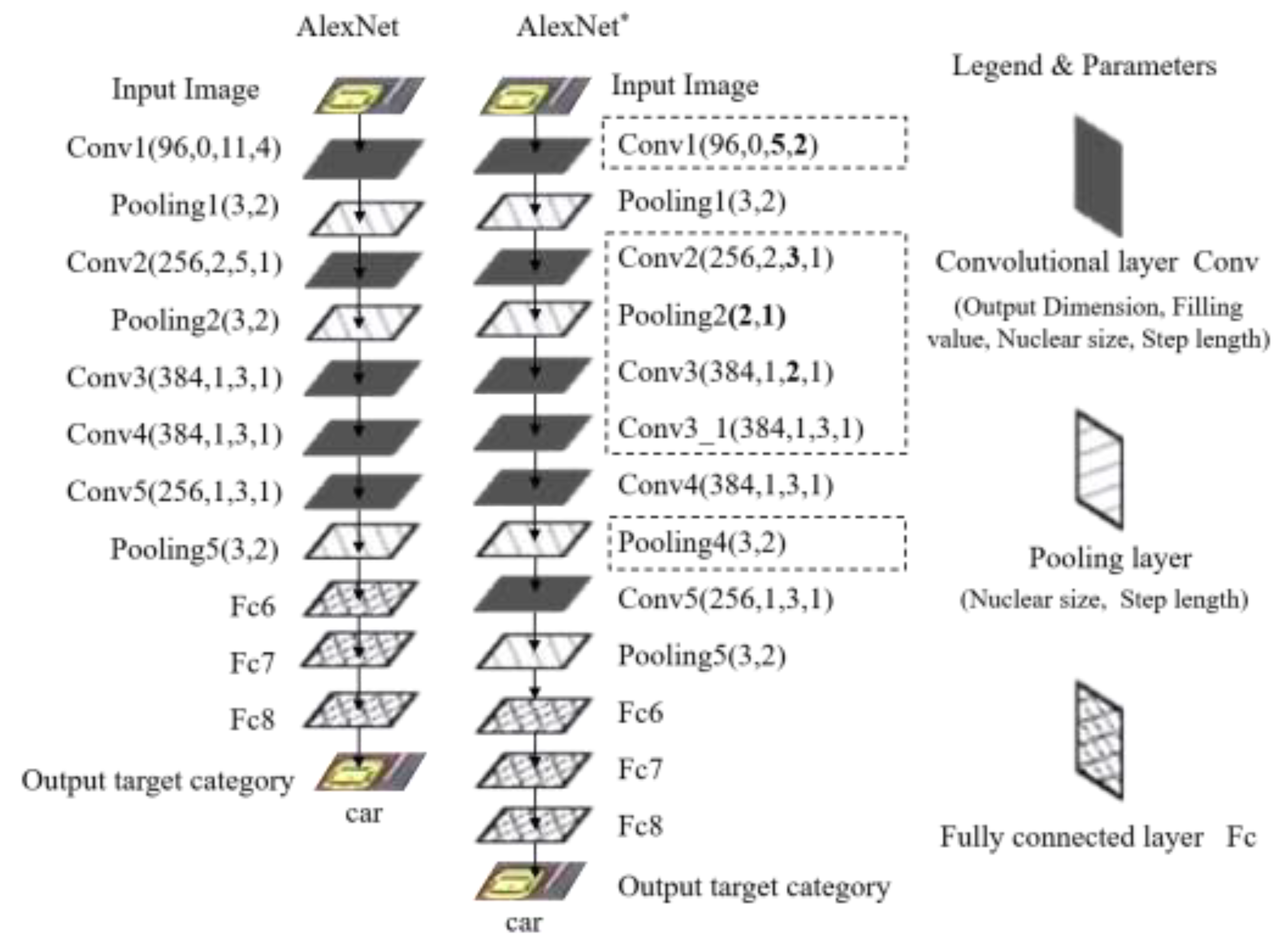
• Deep learning model construction and test: the AlexNet was used as the prototype. The deep learning model was reconstructed by optimizing the convolutional network parameters and adding convolutional and residual layers. Thereafter, the reconstructed deep learning model was trained and tested with feedback optimization.
• Reconstructed deep learning model performance evaluation: the multiple reconstructed deep learning models were constructed as alternatives and the optimal model that met the precision requirement was selected. The optimal model could identify the candidate vehicle target type (bus, car, or non-vehicle) and localize it in the original image. The details of the proposed detection framework are shown in Figure 1.

2. Methodologies

2.1. UAV High-Resolution Video Vehicle Target Pre-Detection

UAV images show more specific scale variations than natural images. The objects in UAV images tend to be denser and smaller because they were taken at high altitudes. However, vehicles have more obvious edge and contour morphological features. If we achieved the accurate detection of vehicle contour in UAV overhead video, it could be applied to the model recognition improvement.

With the continuous development of gimbal and vibration reduction technology, UAV video can avoid the situation of shaking effectively. Because the wide-area scene of a hovering UAV video is relatively stable, it is necessary to outline the region of interest (ROI) through human processing, and the subsequent detection only needs to expand the operation on this ROI. The method not only reduced the number of operations and saved running time, but also improved the detection results, as shown in Figure 2. Then, grayscale images synthesized the information of each red–green–blue color mode (RGB) channel of the true color bitmap, which could make image processing more convenient and efficient [17]. Therefore, the color image was converted to a grayscale image based on the established video maturity analysis algorithm, as in Figure 3, where the rectangular wireframe range is ROI.

2.2. Skeleton Image Skeleton Analysis and Processing

Canny edge detection was performed on the grayscale processed image ROI. A sub-pixel skeleton was generated based on the edge-pixel center sub-pixel. Then, the image skeleton was decomposed into arc segments by the polygon approximation algorithm. If the distance between the endpoints of any adjacent arc segments was less than a threshold value [18], then the endpoints of the arc segments were connected, and the skeleton reconstruction image was obtained.

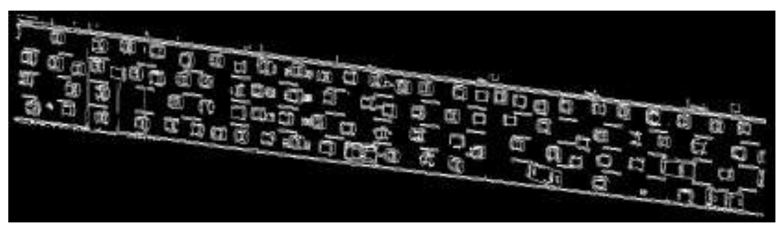
2.2.1. Canny Edge Detection

The Canny edge detection algorithm is a widely used classical edge detection algorithm, while the traditional algorithm has problems such as poor continuity and unclear edge detection results. Based on this, we divided the algorithm into four main steps as follows:

(1)

Eliminate image noise with Gaussian filtering. The basic principle of Gaussian smoothing is to recalculate the value of each point in the image. When calculating, the weighted average of the point and its adjacent points is taken, and the weight fits the Gaussian distribution. It can suppress the high-frequency part of the image, and let the low-frequency part pass through [19].

(2)

Image gradient intensity and direction were obtained by convolution with the Sobel operator convolution. Sobel operator is the weighted difference between the gray values of the upper, lower, left, and right fields of each pixel in the image and reaches the extreme value at the edge to detect the edge. It has a smooth suppression effect on noise and has a good detection effect [20].

(3)

The non-maximum suppression technique was used to retain the maximum value of the gradient intensity at each pixel and delete the other values.

(4)

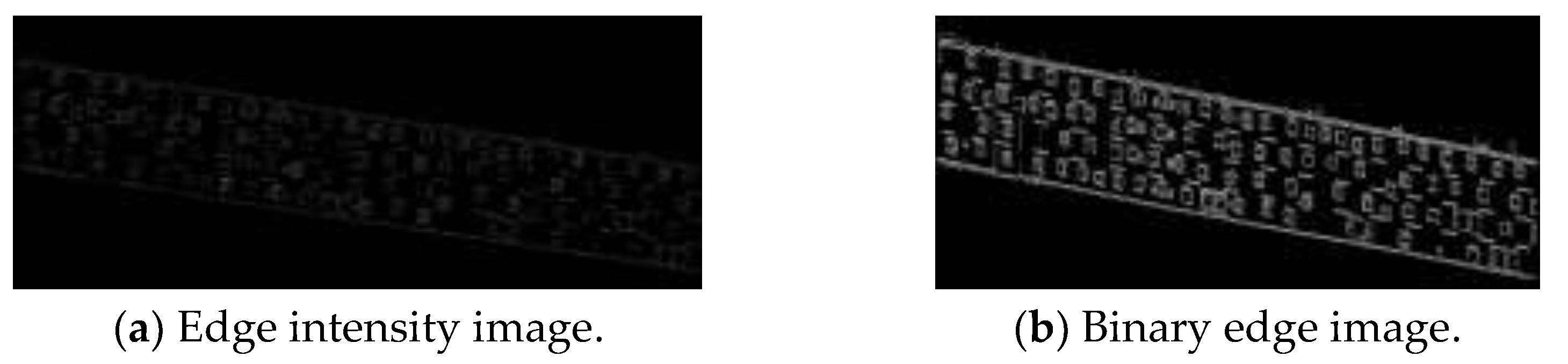
Image weak edge and strong edge were defined by double thresholding, and edge-connected processing was performed to obtain edge images.

Taking the grayscale image of Figure 3 as an example, Canny edge detection was performed on the ROI to obtain the edge intensity image; then, the simple threshold segmentation method or OTSU segmentation method was used to obtain the binary edge image, as in Figure 4a,b. The idea of the OTSU segmentation is to maximize the variance between classes. The original image can be divided into the foreground and background images by the OTSU segmentation [21].

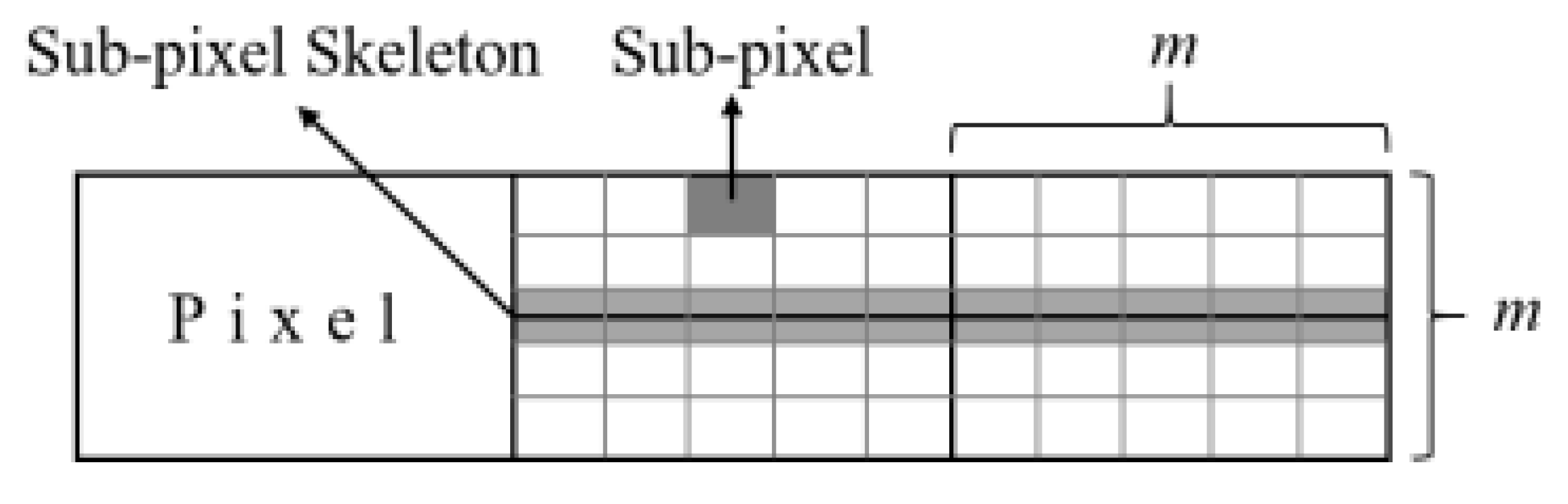
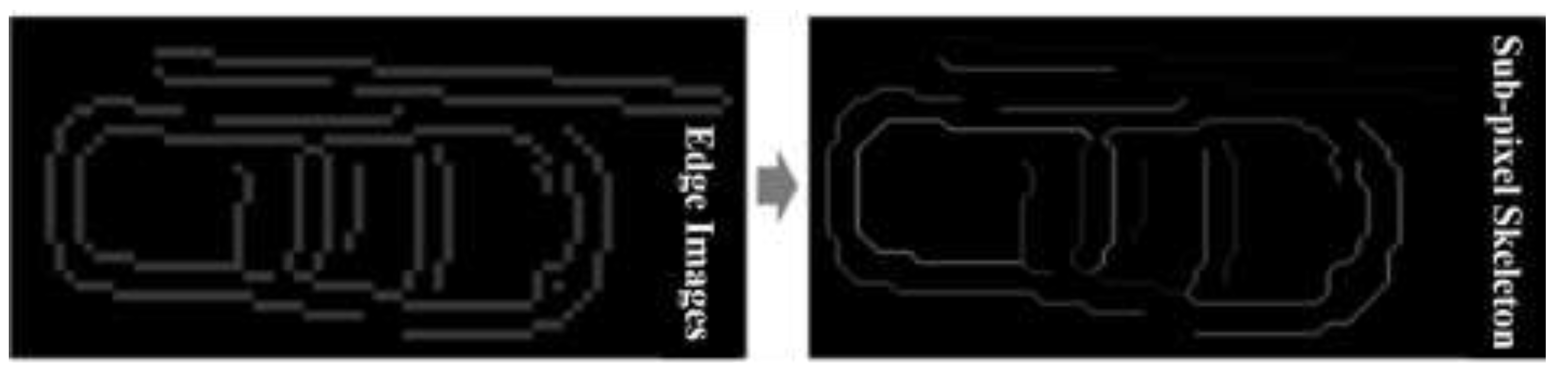
2.2.2. Skeleton Image Generation

Sub-pixel image processing allows for greater utilization of image information. To generate sub-pixel-level skeleton images, the skeleton of ROI edge images was decomposed and reconstructed. The sub-pixel is shown in Figure 5.

Each physical pixel can be divided into $m\times m$ sub-pixels. The line width in the ROI edge image is 1 px. As shown in Figure 5, the central sub-pixel of each pixel was connected to form the sub-pixel skeleton. Then, taking the first candidate vehicle region in the upper left corner of the ROI edge image in Figure 4 as an example, its sub-pixel skeleton is generated in Figure 6.

2.2.3. Skeleton Image Decomposition

The subpixel skeleton was decomposed into straight-line segments or arc segments by the Ramer polygon approximation algorithm. The algorithm can approximate a curve as a series of points and reduce the number of points, making contour edges more precise [22]. The main steps are:

(1)

Assigning several points along the edge as initial points and connecting the initial points to form the initial polygon.

(2)

Between any two neighborhood breakpoints, along the skeleton curve segment, the point with the greatest vertical distance from the line formed by the two breakpoints was found. If the distance satisfies d > d₁, then the point would be used as a new breakpoint to continue the segmentation.

(3)

Continue to decompose the skeleton until all the threshold conditions d ≤ d₁ are met.

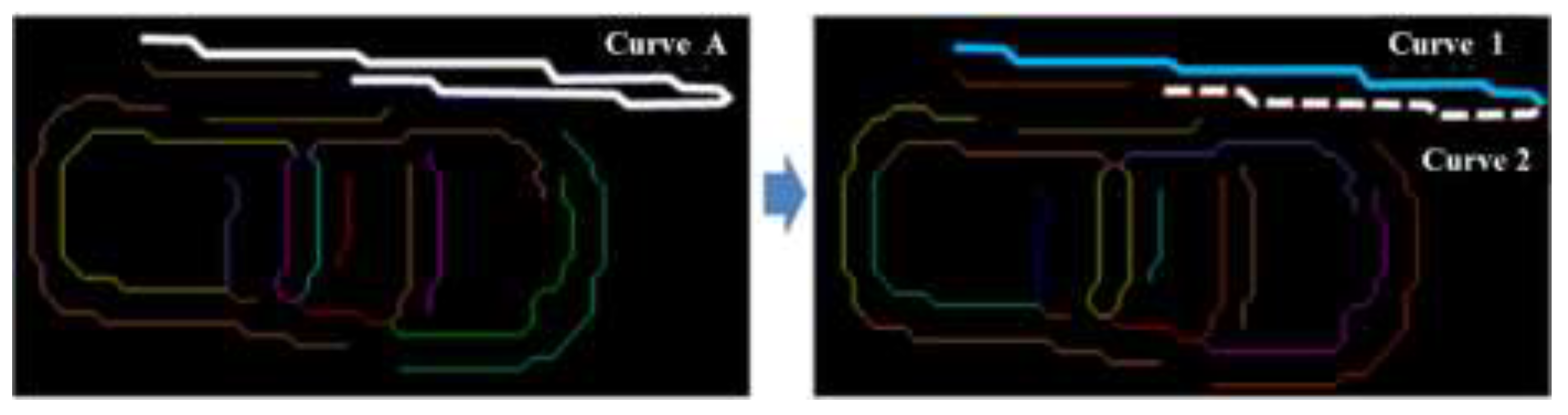
(4)

We assumed that the threshold d₂ is d₂ < d₁. Then, with d₂ as the threshold, refer to steps (1)–(3) for segmentation. Eventually, the decomposition result of the skeleton was obtained. Figure 7 shows an example of the result of skeleton decomposition; Curve A in Figure 7 was decomposed into Curve 1 and Curve 2.

The pseudo-codes of the skeleton decomposition Algorithm 1 from step (1) to (3) are as follows (step (4) is similar, so it will not be repeated here) [23]:

Algorithm 1: Image skeleton decomposition algorithm (“←” means assignment)

①: int SkeletonNumber←The number of curves in the skeleton image;

②: int d1←Distance thresholds;

③: For int i = 1 to SkeletonNumber;

④: Curve[i]←The i-th skeleton curve;

⑤: InitPt[]←The initial set of breakpoints for Curve[i];

⑥: Line[]←The set of line segments formed by any initial breakpoint;

⑦: maxDist←The maximum vertical distance between Curve[i] and ∀ Line;

⑧: pTemp←The point on Curve[i] that generates maxDist;

⑨: If maxDist > d1;

⑩: Split Curve[i] from breakpoint pTemp;

⑪: InitPt[]=Merge{InitPt[], pTemp}// Adding new breakpoints;

⑫: return to ⑤//Enter the ⑤ loop operation;

⑬: Else;

⑭: i++//Segmentation of the next skeleton curve;

⑮: End For

According to the results of skeleton decomposition, for any adjacent skeleton curve, if its endpoint distance was less than the threshold d₃, then the two endpoints were connected. The processing result is shown in Figure 8. The skeleton connection processing can effectively enhance the closure, continuity, and integrity of the candidate target image structure, which helped vehicle recognition. Since the skeleton connection result was still a sub-pixel level image, to facilitate the subsequent work on vehicle recognition and to reduce the computational cost, it was necessary to reduce it to a pixel-level image (Figure 8). According to the ROI edge image in Figure 2, the pixel-level skeleton image obtained after processing is shown in Figure 9.

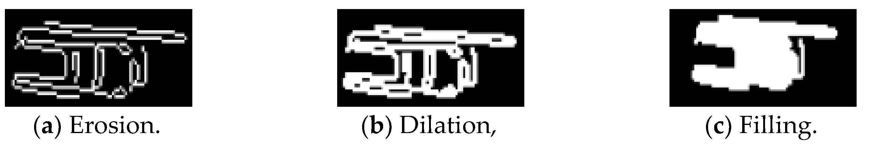
2.3. Morphological Detection

We performed a dilation filling operation on the skeleton image to obtain the original connected domain image. Four morphological operators were mainly used to process the reconstructed skeleton images: dilation, erosion, filling, and closing operations [24]. Meanwhile, the vehicle targets were extracted by combining various morphological features, such as the area of the connected domain, the rectangularity, and the long and short axes of the equivalent ellipse.

First, we used morphological operators for the connected domain feature extraction work. Morphological operators are widely used to extract image components from images that are useful for expressing and depicting the shape of regions, and they have good results in the analysis and processing of image shape and structure [25]. Morphological operators are introduced to study the characteristics of a vehicle’s contour-connected domain, which can be divided into four types: dilation, erosion, filling, opening, and closing. Dilation used t × t structural elements to expand the boundary of the target area to the outside, which could be used to fill some gaps in the image region. Erosion was in contrast to dilation, which used t × t structuring elements to shrink the boundary of the target area inward, thereby eliminating small and meaningless objects. The process of the first dilation and then erosion is called a closing operation, which can be used to fill small holes in objects, connect adjacent objects, and smooth boundaries. The filling is to fill out the area enclosed by the outline to eliminate voids and gaps inside the object, as shown in Figure 10. Figure 10a is the erosion effect of the middle figure, on the contrary, Figure 10b is the dilation effect of Figure 10a,c is the filling effect of Figure 10b. The effect of the closing operation is shown in Figure 11.

Furthermore, the connected domain has the following morphological characteristics. A pixel is the smallest unit of an image. Each pixel is surrounded by eight adjacent pixels. There are two common adjacencies: 4-adjacency and 8-adjacency. As in Figure 12, the adjacency includes points at the top, bottom, left, right, and diagonal positions. According to the 4-adjacency or 8-adjacency, the region formed by connected pixels is called the connected domain. In image processing, computational analysis of connected domains is often carried out to achieve image segmentation, noise removal, and target recognition. The connected domains were built based on 8-adjacency and the calculation and analysis of morphological characteristics such as area, rectangularity, and equivalent ellipse with major and minor axes were performed.

(1)

Area, S: the total number of pixels in the connected domain.

(2)

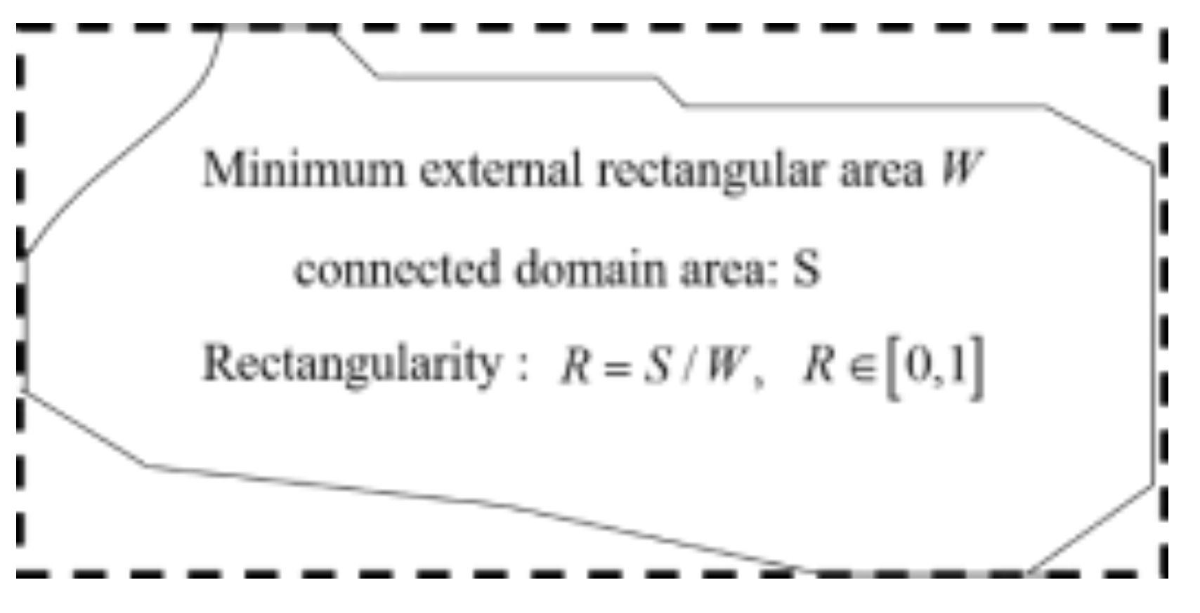
Rectangularity, R: the ratio of the connected domain area S to the minimum external rectangular area W, reflects the fullness of the connected domain area to its outer rectangle, as shown in Figure 13.

(3)

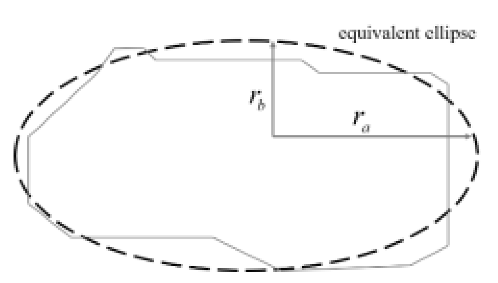
Equivalent ellipse with major and minor axes [26]: a corresponding ellipse can be obtained for each connected domain; the elliptic equation is in the same form as the moment of inertia in the connected domain. Assuming that an ellipse region is homogeneous and has the same moment of inertia as the connected domain, the ellipse parameters can reflect the characteristics of the aforementioned connected domain. This ellipse is called an equivalent ellipse. Accordingly, the major axis r_a and minor axis r_b of the equivalent ellipse can be solved, as shown in Figure 14.

Second, we recognized the vehicle based on the vehicle recognition algorithm of morphological analysis, including the following four steps:

(1)

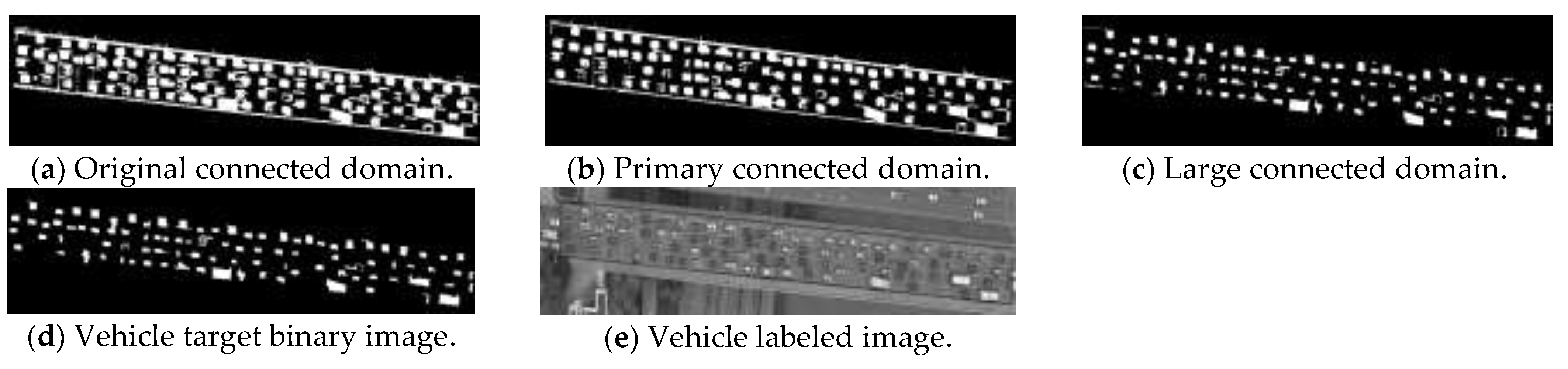
Connected domain screening: The dilation and filling operations were performed on the skeleton reconstruction image to obtain the connected domain image. The results are shown in Figure 15a. Based on the connected domain rectangularity, area, and equivalent elliptic minor axis thresholds, the connected domains that satisfied conditions (1)–(3) were extracted. As shown in Figure 15b, this step removes some small areas and narrow lanes markings.

$$d_1\le D\le d_2$$

(1)

$$A>s_1$$

(2)

$$b_1\le b\le b_2$$

(3)

where $D$, $A$, and $b$ are the rectangularity, the area, and the equivalent elliptic short axis length of the connected domain, respectively. $d_1$, $d_2$, $s_1$, $b_1$, and $b_2$ are threshold parameters ($d_1=0.1$, $d_2=1$, $s_1=50$, $b_1=5$, and $b_2=200$, respectively, in this paper).

(2)

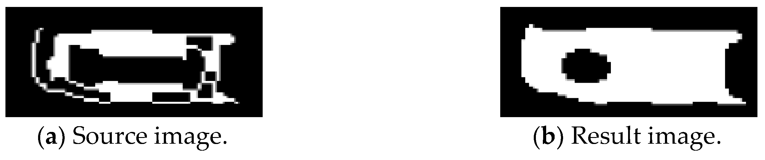
The larger connected domain was chosen based on the area and equivalent elliptic major axis and minor axis thresholds. If condition (4) is satisfied, then perform the closing operation and dilation operation on it; the results are shown in Figure 15c. Next, the smaller connected domain was chosen. If condition (5) is satisfied, perform the opening operation and dilation operation on it. This step effectively divides the large, connected domain and further eliminates narrow lane markings and road edges, as shown in Figure 15c.

$$A>s_2 \mathrm{or} a>a_1$$

(4)

$$A<s_3 \mathrm{or} b<b_3$$

(5)

where $a$ is the length of the equivalent elliptic major axis in the connected domain; $a_1$, $b_3$, $s_2$, and $s_3$ are threshold parameters ($a_1=30$, $b_3=15$, $s_2=1500$, and $s_3=600$, respectively); and the rest of the symbols have the same meaning as before.

(3)

According to the area and equivalent ellipse minor axis threshold, if condition (6) is satisfied, perform the opening operation and dilation operation on it. Finally, all subblocks were converted to rectangular subblock results.

$$A>s_2 \mathrm{or} a>a_1$$

(6)

where $b_4$ and $s_4$ are threshold parameters ($b_4=10$ and $s_4=500$, respectively), and the rest of the symbols have the same meaning as before.

(4)

Extract the rectangular subblock coverage area images as candidate targets, as shown in Figure 15d,e.

In summary, the algorithm mainly uses morphological operations to perform line-to-plane conversion on the skeleton structure image, and then calculates and analyzes the morphological features of the connected domain, and finally identifies the vehicle, as shown in Figure 16. The pseudo codes of the vehicle recognition Algorithm 2 for steps (1)–(4) are as follows [27].

Algorithm 2: Vehicle recognition algorithm based on morphological analysis (“←” means assignment):

①: Skeleton←skeleton reconstruction image;

②: Image0←Dilation and filling of Skeleton;

③: R[i], A[i]←The rectangularity, area of the ith connected domain;

④: ra[i], rb[i]←The length of the major axis, the length of the minor axis of the equivalent ellipse of the ith connected domain;

⑤: For int i = 1 to M//M is the number of concatenated domains of Image0;

⑥: If R[i]∈[r1,r2] or A[i] > s1 or rb[i]∈[b1, b2];

⑦: Retain the ith connected domain of Image0 // r1, r2, s1, b1, b2 are threshold parameters;

⑧: End For//Let be Image1;

⑨: For int j = 1 to N//N is the number of connected domains of Image1;

⑩: If A[j] > s2 or ra[j] > a2//s2, a2 is the threshold parameter;

⑪: Closing operation and erosion operation on the jth connected domain of Image1;

⑫: End For//The first large target segmentation result is obtained, let it be Image2;

⑬: Image3 ← The result of the dilation process of Image2;

⑭: s3←Connected domain area threshold parameter;

⑮: a3←The length threshold parameter of the major axis of the equivalent ellipse of the connected domain;

⑯: Return to ⑨~⑪//Image3 is processed with thresholds s3 and a3 // the result is named Image4;

⑰: For int k = 1 to W//W is the number of connected domains of Image4;

⑱: If A[k] < s4 or rb[k] < b3 or rb[k] > b4;

⑲: Remove the kth connected domain//s4, b3, b4 are the threshold parameters;

⑳: End For//The binary image of vehicle recognition is obtained.

2.4. AlexNet Model

We chose the AlexNet to be the prototype deep learning model. It consists of 5 convolutional layers, 3 pooling layers, and 3 fully connected layers, as shown in Figure 17. AlexNet has contributions in using rectified linear units (ReLU) nonlinearity activation function, using local response normalization (LRN) to smooth the output; first using graphics processing unit (GPU) acceleration training; and using the dropout method to randomly inactivate neurons in proportion to reduce overfitting in the first two layers of the fully connected layer, etc. The convolution part is divided into two parts for calculation by grouping. Split-channel learning reduces the learning dimension of the convolution kernel. The higher the dimension of the convolution kernel, the higher the difficulty of learning.

3. Data Set

3.1. Experimental Data

The raw data of the UAV video came from the traffic video shot at a height of 200–250 m above the ground in the main urban roads of Chongqing, and the video resolution is 3840 pixels × 2160 pixels. The dataset was produced using the VOC2007 standard. For UAV video vehicle detection, the production of VOC2007 dataset mainly includes:

(1)

JPEGImages folder: store training images, verification images, and test images.

(2)

Annotations folder: store the xml format information file corresponding to each image, including the image file name, image size, vehicle annotation outline information, etc.

(3)

ImageSets folder: store txt files containing image category labels, and record the image names used for training, validation, and test in train.txt, val.txt, and test.txt files, respectively.

3.2. Deep Learning Image Benchmark Library Construction

Deep learning models require a large number of measured images for training, testing, and verification. In order to establish and optimize the deep learning model for UAV video vehicle recognition, a benchmark library including candidate target images, training images, test images, and verification images was constructed. Since the main urban area of Chongqing has implemented the restriction management of trucks, considering the actual demand for traffic control on urban arterial roads and the operation characteristics of vehicles, the extracted vehicle candidates from the UAV video can be manually classified into bus categories, car categories, and non-vehicle category, which are marked as bus, car, and non_vehicle, respectively, to form a candidate set. Car categories include mini car, sport utility vehicle (SUV), van, etc. Non_vehicle includes lane lines, trees, railings, other traffic signs, etc. To ensure the sample size and sample class balance, color dithering and rotation transform dilation were performed on the candidate set images. Meanwhile, the size normalization, grayscale conversion, classification label making, lightning-memory-mapped database (LMDB) data files, and mean.binaryproto files were preprocessed. Then, a relatively independent training set, test set, and validation set were formed. The number of sample images in each part of the image benchmark library is shown in

Table 1. Sample Sizes of the benchmark image library.

Category	Candidates	Training	Test	Validation
bus	5152	10,000	3000	50,000
car	34,699	10,000	3000	50,000
non_vehicle	15,669	10,000	3000	50,000
Total	55,520	30,000	9000	150,000

. Accordingly, we obtained the VOC2007 UAV video image benchmark library with the training sets of 3 types of candidate targets: 10,000 images, the test set of 3000 images, and the validation set of 50,000 images.

3.3. Test Environment

The experimental platform is a workstation with a 64-bit Windows 7 operating system. Memory is 16 GB + GPU Nvidia GTX960 + Intel Core i5-4590. Microsoft Visual Studio 2010 + OpenCV2.4.9 environment was configured to build the deep learning framework of Windows version Caffe, and Python 3.6 was used as the programming language

4. Experiments and Analysis

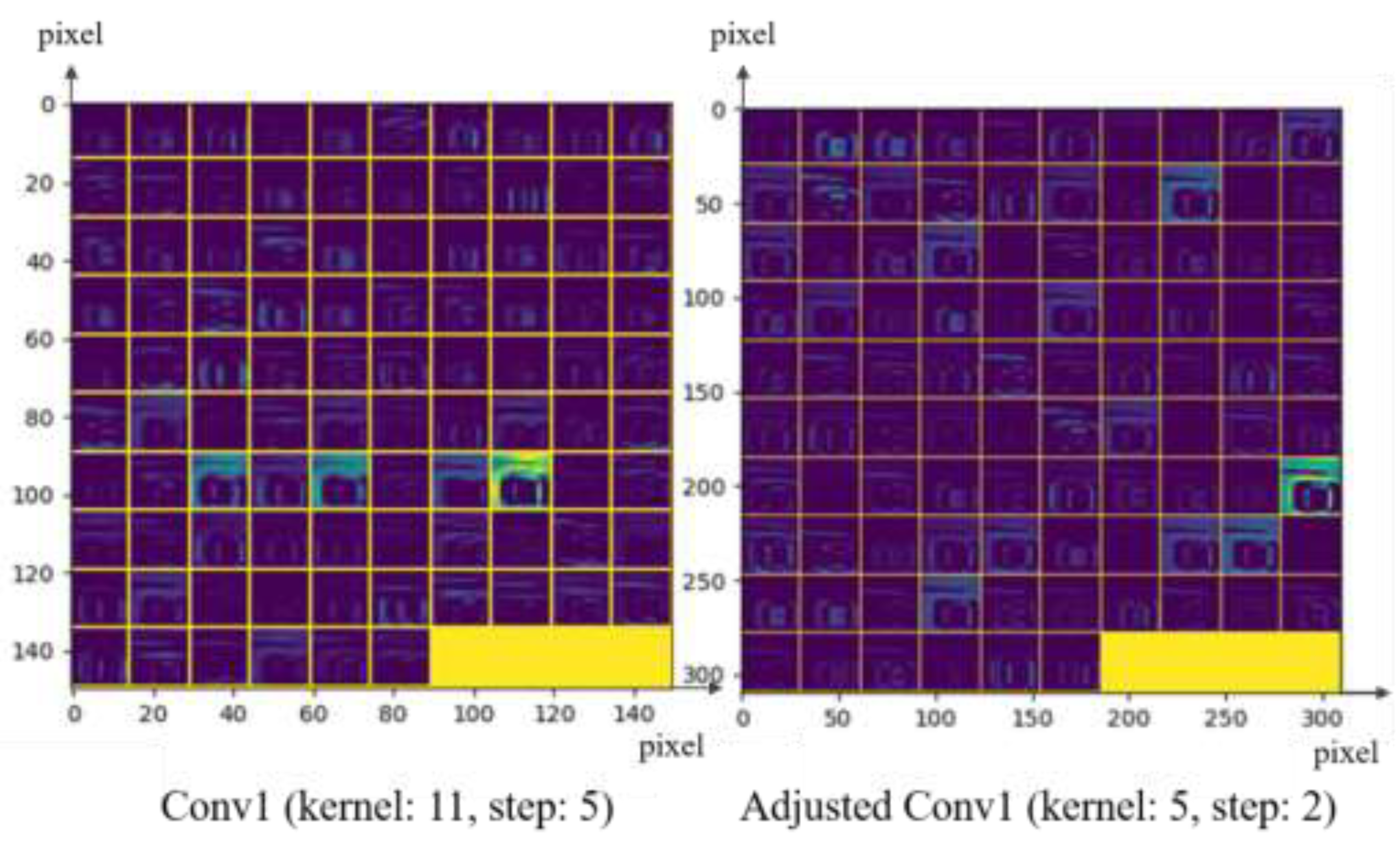
4.1. AlexNet Model Improvement

The main structure of AlexNet comprises five convolutional layers, three pooling layers, and three fully connected layers. The convolution layer mainly extracts image features; the pooling layer reduces the size of the image matrix to reduce the fully connected layer parameters. The fully connected layer mainly performs data normalization and image classification. Additionally, the AlexNet model improvement method generally adjusts the number and parameters of convolutional layers and pooling layers. Due to the small scale of vehicle targets in high-altitude scenes for UAV video images, some measures can be taken to improve the recognition effects. For instance, adopt a smaller convolution kernel size to obtain more vehicle features, add more convolutional layers at appropriate locations, and deepen the network depth to help extract more abstract image features. Moreover, add a pooling layer to achieve feature image dimensionality reduction, reduce computational effort, and speed up the convergence of the model. For example, after adjusting the convolutional layer, the vehicle contour information can be better extracted, as shown in Figure 18.

We carried out AlexNet improvement experiments through the network structure and parameter adjustment mentioned above. Each model was trained and tested 100,000 times using the training and test set images to obtain its change of $F_1$ compared with AlexNet. Then, several cross experiments, such as adjusting convolution parameters, adding and subtracting convolution layers, adding pooling layers, and adding residual layers, were conducted.

Table 2. Changes of improved AlexNet models under different adjustment methods.

Experimental Model	Adjustment Method	$\mathbf{\Delta }{\mathit{F}}_{\mathbf{1}}$ (Bus)	$\mathbf{\Delta }{\mathit{F}}_{\mathbf{1}}$ (Car)	$\mathbf{\Delta }{\mathit{F}}_{\mathbf{1}}$ (Non_Vehicle)	$\mathbf{\Delta }{\mathit{F}}_{\mathbf{1}}$ Mean Value
AlexNet1	Reduce the first two layers of convolution kernels; add Conv3_1 after Conv3.	0.48%	−13.46%	−7.39%	−6.79%
AlexNet2	Reduce the first two layers of convolution kernels; add Conv4_1 after Conv4.	−2.32%	−22.24%	−9.82%	−11.46%
AlexNet3	Reduce the first three layers of convolution kernels; add Conv4_1, Pooling4 after Conv4.	2.42%	1.32%	0.91%	1.55%
AlexNet4	Reduce the first three layers of convolution kernels; add Conv3_1 after Conv3.	0.55%	−1.52%	−1.54%	−0.84%
AlexNet5	Add residual layer “res” after Conv5.	−2.68%	−5.57%	−0.13%	−2.79%
AlexNet*	Reduce the first three layers of convolution kernels; add Conv3_1 after Conv3; add Pooling4 after Conv4.	2.85%	3.27%	2.80%	2.97%

shows the representative experimental model metrics, see later for details of the calculation method. This paper finally proposed an improved AlexNet model (named AlexNet*), which mainly optimized some convolution parameters and pooling parameters on the basis of AlexNet, and added one convolution layer and one pooling layer. As shown in Figure 19, the dotted box means the improvement section.

As mentioned earlier, the AlexNet model improvement requires several cross experiments such as adjusting convolution parameters, adding convolution layers, adding pooling layers, adding residual layers, etc. Therefore, this paper also proposed several improved models before establishing AlexNet*. Training, test, precision, recall, and $F_1$ value calculations were performed similar to AlexNet* for each model to obtain its $F_1$ value increment compared with AlexNet. The results are shown in Table 2.

By the change in the $F_1$ values of AlexNet6, it can be found that the introduction of the residual layer reduces the model performance. Comparing AlexNet1 with AlexNet2, it can be seen that adding the convolutional layer after Conv3 is more conducive to model improvement than adding it after Conv4. By comparing AlexNet2 and AlexNet3, it can be seen that, for UAV video vehicle detection, appropriately reducing convolution parameters and adding pooling layers can help improve the performance of the model. Comparing AlexNet* and AlexNet5, it was found that the introduction of the pooling layer Pooling4 is helpful for the performance improvement of the model. Comparing AlexNet* with AlexNet4, we can see that after adding two successive layers of convolution behind Conv3, the model performance drops significantly, with a 17.29% reduction in $F_1$. In summary, we reduced the first three layers of the convolution kernel of the AlexNet model to be smaller and added only one layer of convolution Conv3_1 after Conv3, and then added the pooling layer Pooling4 after Conv4 to optimize the AlexNet model, which finally improved the mean $F_1$ value of AlexNet* by 2.97%.

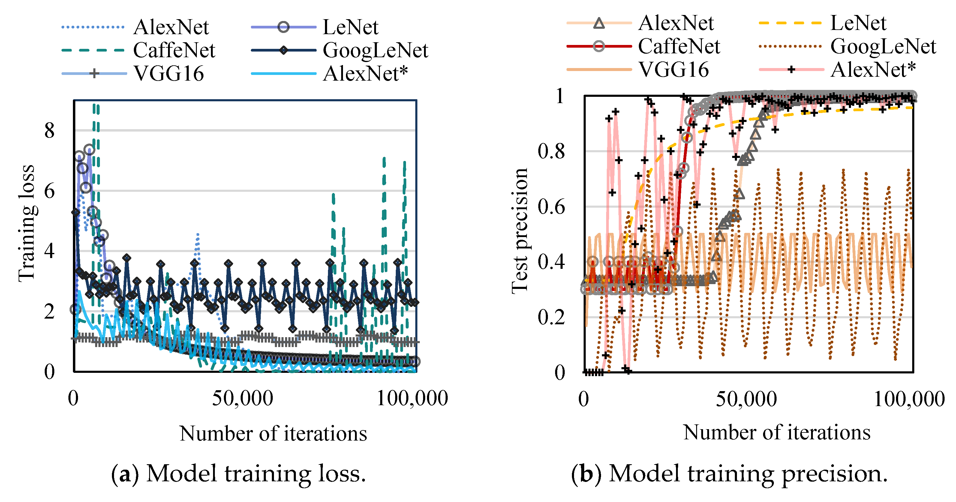
4.2. Model Training

In this paper, the commonly used AlexNet, LeNet, CaffeNet, GoogLeNet, VGG16, and AlexNet* were trained and tested. The main parameter include test_interval, base_lr, max_iter, lr_policy, gamma, and solver_mode, and their settings are shown in

Table 3. Parameters of each model.

	AlexNet	LeNet	CaffeNet	GoogLeNet	VGG16	AlexNet*
Test_Interval	500	1000	300	100	100	100
Base_lr	0.001	0.0001	0.001	0.001	0.0001	0.0001
Max_iter	100,000	100,000	100,000	100,000	100,000	100,000
lr_Policy	inv	inv	inv	Step	Step	inv
Gamma	0.001	0.0001	0.0001	0.001	0.01	0.0001
Solver_Mode	GPU	GPU	GPU	GPU	GPU	GPU

. Each model is trained for 100,000 iterations based on the training set and test set images. During this process, the network parameters will be fine-tuned with the goal of minimizing the loss value until the loss value converges and reduces to an acceptable range. After training, if the loss value of the two types is closer to 0 and the precision is closer to 1, the model training effect is better.

The training results are shown in Figure 20. It can be seen that the training loss of AlexNet*, LeNet, and AlexNet started to gradually decrease and eventually converged to 0 at about 50,000 iterations; VGG16 and GoogLeNet oscillated more seriously and failed to converge, while CaffeNet showed signs of convergence at 50,000–70,000 iterations, but stronger oscillations occur after 70,000 iterations, as shown in Figure 20a. For test loss and test precision, VGG16 and GoogLeNet oscillated severely failing to converge, while AlexNet, LeNet, CaffeNet, and AlexNet* all oscillated in the previous 50,000 iterations, but then their test loss values gradually converged to 0, and the test precision gradually increased during the oscillation and finally stabilized at 0.9~0.96. This shows that AlexNet, LeNet, and AlexNet* have the best training results, CaffeNet is not outstanding, and VGG16 and GoogLeNet are worse, as shown in Figure 20b.

4.3. Comparative Analysis between AlexNet* and Traditional CNN Models

4.3.1. Evaluation Indicators

The data was from the test images set. For certain types of targets (car, bus, non_vehicle), recognition results can be divided into four cases:

(1)

$T_{\mathrm{P}}$: the number of targets that have been correctly identified;

(2)

$F_{\mathrm{N}}$: the number of targets that have been identified as other objects;

(3)

$F_{\mathrm{P}}$: the number of other objects that have been detected as targets;

(4)

$T_{\mathrm{N}}$: the number of non-target objects that have been recognized as targets.

The precision, $P$, recall, $R$, and the comprehensive evaluation index, $F_1$, were calculated based on $T_{\mathrm{P}}$, $F_{\mathrm{N}}$, $F_{\mathrm{P}}$, and $T_{\mathrm{N}}$, as shown in Equation (7). The quality of the model was evaluated according to $F_1$: the higher the $F_1$, the better the method will be.

$$F_1=\frac{2PR}{P+R}$$

(7)

where $P=T_{\mathrm{P}}/(T_{\mathrm{P}}+F_{\mathrm{P}})$, $R=T_{\mathrm{P}}/(T_{\mathrm{P}}+F_{\mathrm{N}})$.

4.3.2. Comparison and Evaluation of AlexNet* and Common Models

The commonly used AlexNet, LeNet, CaffeNet, GoogLeNet, VGG16, and AlexNet* were tested, and the tested performance indicators are shown in

Table 4. Verification results of models.

Models	Bus Evaluation Indicators (%)			Small Car Evaluation Indicators (%)			Non-Vehicle Evaluation Indicators (%)			${\mathit{F}}_{\mathbf{1}}$ Average (%)
	$\mathit{P}$	$\mathit{R}$	${\mathit{F}}_1$	$\mathit{P}$	$\mathit{R}$	${\mathit{F}}_{\mathbf{1}}$	$\mathit{P}$	$\mathit{R}$	${\mathit{F}}_{\mathbf{1}}$
AlexNet	91.28	86.77	88.97	71.19	88.16	78.77	89.19	72.33	79.88	82.54
LeNet	98.41	54.66	70.28	51.52	72.71	60.31	60.08	62.08	61.06	63.88
CaffeNet	52.25	91.95	66.63	52.90	56.72	54.75	64.38	10.84	18.55	46.64
GoogLeNet	4.62	5.63	5.07	29.64	52.65	37.93	12.40	0.06	0.12	14.38
VGG16	0.00	0.00	0.00	33.33	100.00	50.00	0.00	0.00	0.00	16.67
AlexNet*	88.65	95.22	91.82	79.91	84.29	82.04	88.80	77.35	82.68	85.51
AlexNet*- AlexNet	−2.63	8.45	2.85	8.72	−3.87	3.27	−0.39	5.02	2.80	2.97

. The comparison and evaluation between AlexNet* and AlexNet found the following:

(1)

The precision of car recognition of AlexNet* was 79.91%, 8.72% higher than AlexNet ($P$= 71.19%). The precision of bus and non-vehicle recognition of AlexNet* were 88.65% and 88.80%, respectively, 2.63% and 0.39% lower than these of AlexNet ($P$= 91.28%, $P$= 89.19%). Thus, AlexNet* is more accurate for car recognition, while bus and non-vehicle recognition are slightly worse than AlexNet.

(2)

The recall of bus and non-vehicle of AlexNet* were 8.45% and 5.02% higher than AlexNet, respectively, but the recall of car recognition was 3.87% lower. It indicates that AlexNet* is less likely to miss bus and non-vehicle targets, but more likely to miss cars.

(3)

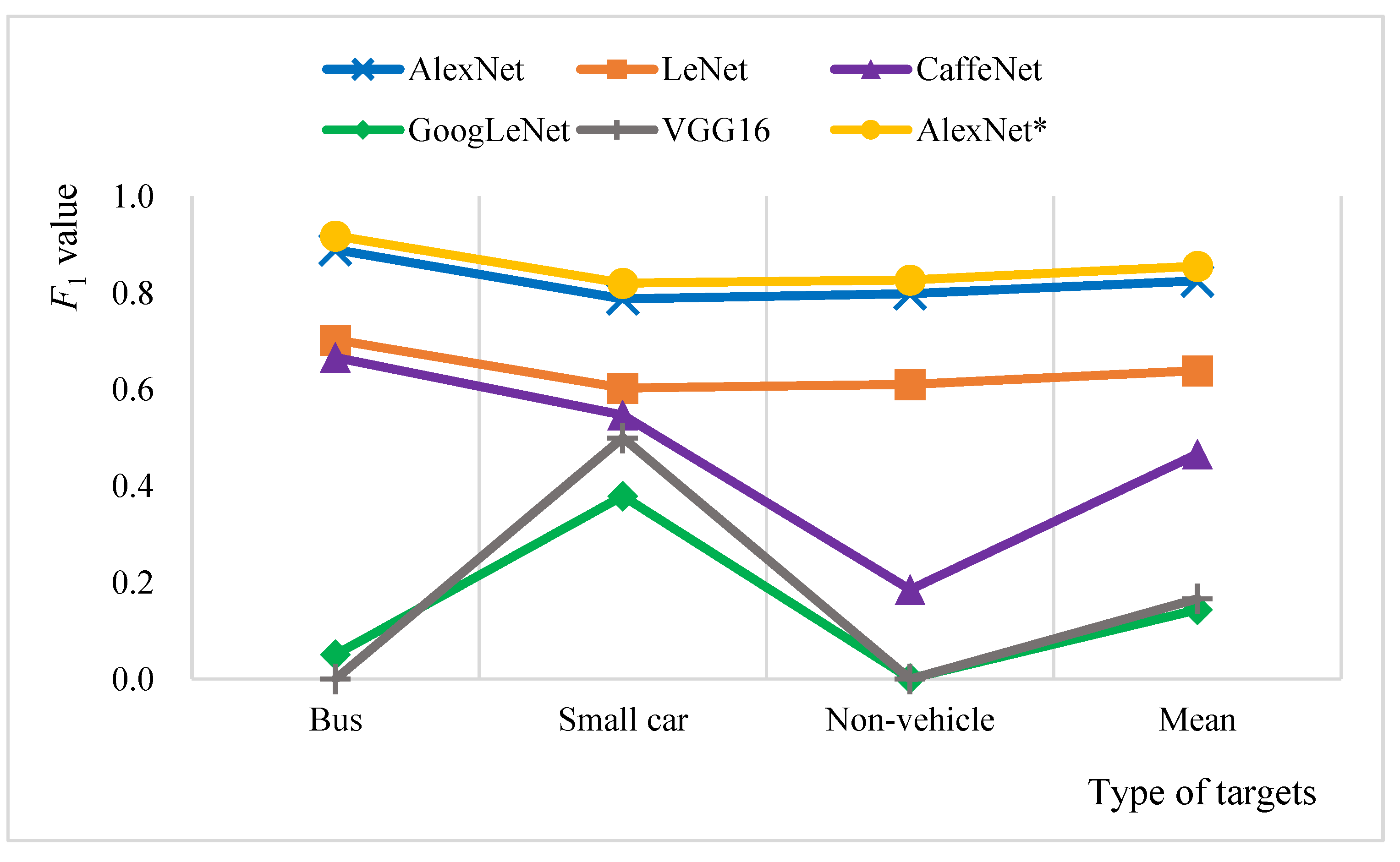
$F_1$ of AlexNet* for the bus recognition (91.82%) was 2.85% higher than that of AlexNet ($F_1$ = 88.97%), and $F_1$ of car and non-vehicles recognition also increased by 3.27% and 2.97%, respectively. Therefore, the comprehensive performance of AlexNet* for all three types of target recognition is better than AlexNet, indicating that the model improvement in this paper produces better results.

The main results for the other models are as follows:

(1)

The precision and recall of LeNet and CaffeNet have no significant differences, but $F_1$ of LeNet (70.28%, 60.31%, 61.06%) are better than CaffeNet (66.63%, 54.75%, 18.55%) for bus, car, and non-vehicle recognitions.

(2)

$F_1$ of GoogLeNet and VGG16 for three types of target recognition are not higher than 50%, largely due to the poor training effect.

Combining the distribution of $F_1$ for each model in Figure 21, it can be seen that the ranking of $F_1$ average is AlexNet* (85.51%), AlexNet (82.54%), LeNet (63.88%), CaffeNet (46.64%), VGG16 (16.67%), and GoogLeNet (14.38%). It indicates that AlexNet* has the best overall performance, with 2.97% improvements over AlexNet.

4.4. Evaluation of Vehicle Test Results

The morphological detection algorithm needs to set three parameters: image segmentation threshold adjustment value Δ, vehicle area threshold a, and vehicle aspect ratio threshold r. On the basis of extensive data test and analysis, the recommended values of Δ = 25, a = 120, and r = 6 were used in the subsequent algorithm evaluation and analysis.

4.4.1. Evaluation Indicators

The data was from the validation images set. For vehicle recognition in each frame of the UAV video, four possible cases were defined in this paper, as shown below:

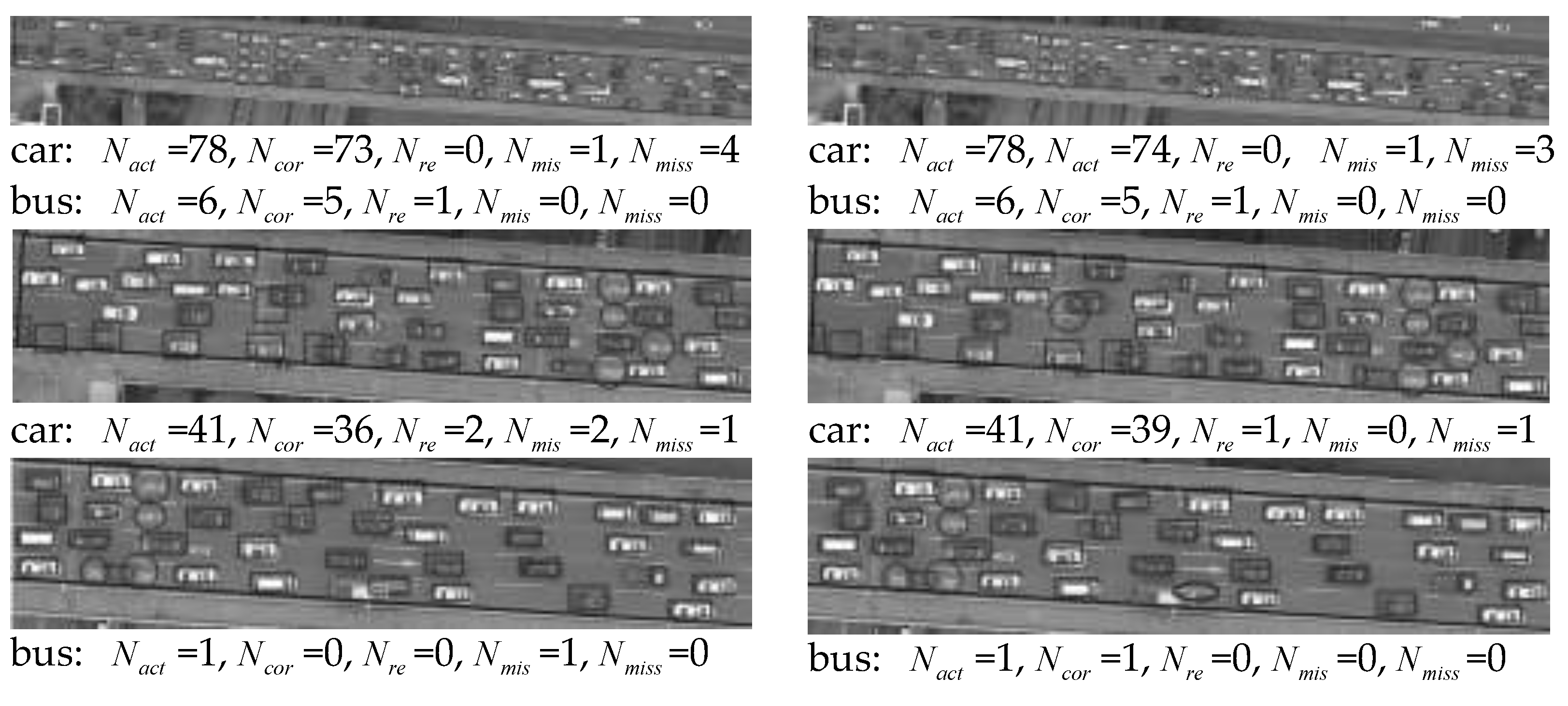
(1)

The vehicle is correctly detected: a vehicle is identified as the correct vehicle category;

(2)

Vehicle misdetection: a vehicle is recognized as another object, $N_{mis}$ denotes the number of vehicles misdetected in a certain frame;

(3)

Vehicle redetection: a vehicle is detected as two or more vehicles, and the detection of large objects (such as buses) is prone to such phenomena;

(4)

Missing vehicle detection.

According to these cases, the algorithmic evaluation indexes of correct detection rate were defined as $P_{cor}$, redetection rate $P_{re}$, and missing detection rate $P_{miss}$, where $P_{cor}$ is equivalent to the aforementioned precision and (1−$P_{miss}$) is equivalent to the recall. The calculations are shown in Equations (8)–(10).

$$P_{cor}=N_{cor}/N_{act}$$

(8)

$$P_{re}=N_{re}/N_{act}$$

(9)

$$P_{miss}=N_{miss}/N_{act}$$

(10)

where $N_{cor}$ is the number of vehicles correctly detected within a given frame; $N_{de}$ is the number of vehicles detected within a given frame, whether correct or not. $N_{miss}$ denotes the number of vehicles missed in a certain frame; $N_{re}$ denotes the number of vehicles repeatedly detected in a certain frame; $N_{act}$ represents the actual number of vehicles within a given frame.

4.4.2. Analysis of Results

A total of 150 frames of detection images were randomly extracted based on the detection results and manual interpretation. Two groups of evaluation index values (precision of the correct detection rate, redetection rate, and missing detection rate) can be calculated for each image before and after algorithm optimization. The statistical results are shown in

Table 5. Evaluation indexes comparison of AlexNet and AlexNet* (sample sizes: 150).

Statistical Values	AlexNet (%)			AlexNet* (%)
	${\mathit{P}}_{\mathit{c}\mathit{o}\mathit{r}}$	${\mathit{P}}_{\mathit{r}\mathit{e}}$	${\mathit{P}}_{\mathit{m}\mathit{i}\mathit{s}\mathit{s}}$	${\mathit{P}}_{\mathit{c}\mathit{o}\mathit{r}}$	${\mathit{P}}_{\mathit{r}\mathit{e}}$	${\mathit{P}}_{\mathit{m}\mathit{i}\mathit{s}\mathit{s}}$
Average	93.10	6.87	6.25	94.63	6.89	4.40
Median	97.02	2.27	2.56	97.65	1.97	1.79
Variance	7.77	7.95	7.30	7.47	7.87	6.18

and Figure 22, in which AlexNet represents the original algorithm and AlexNet* represents the algorithm optimization.

Table 5 shows that the average $P_{cor}$ of the AlexNet algorithm and the AlexNet* algorithm in this paper was 93.10% and 94.63%. AlexNet* had an increase of 1.53% compared with AlexNet, indicating that the AlexNet* algorithm was more capable of correct vehicle recognitions. The average $P_{re}$ of AlexNet and AlexNet* was 6.87% and 6.89%. AlexNet* reduced by 0.02% when comparing with AlexNet. There was almost no difference between the two. The average $P_{miss}$ values were 6.25% and 4.40%, respectively. AlexNet* reduced 1.85% when referring to AlexNet, so the detection results applied AlexNet* algorithm have fewer missed vehicle identifications.

On the basis of the evaluation indicators in Figure 22, the observed results are shown as follows:

(1)

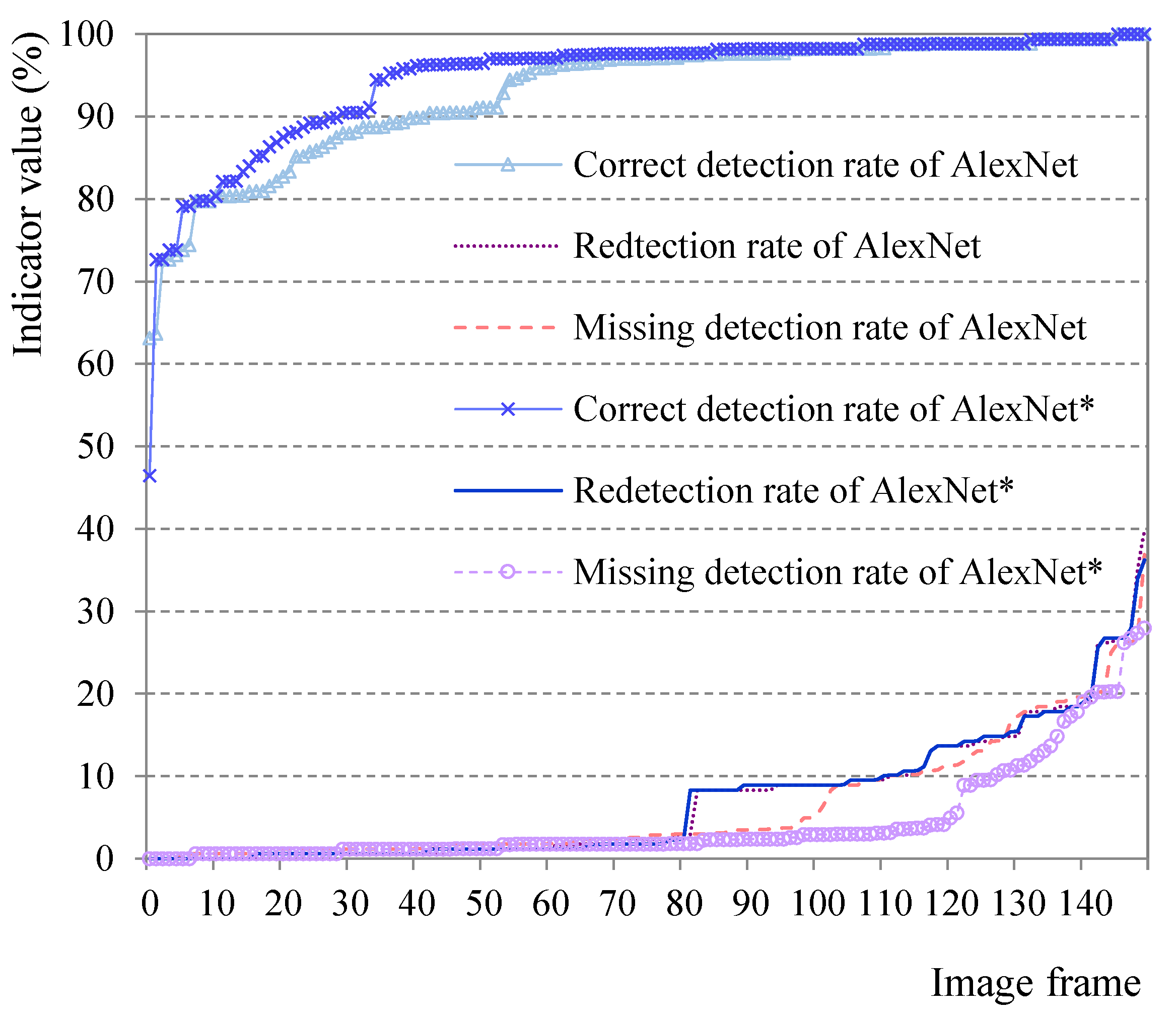
Under the standard that $P_{cor}$ is higher than 90%, the AlexNet* algorithm has 123 images (82% of the total sample), which is higher than the 111 images of the AlexNet algorithm (74% of the total sample). It indicates that $P_{cor}$ of the AlexNet* algorithm has reached a higher level;

(2)

For $P_{re}$ of 150 images, the identification results by AlexNet and AlexNet* algorithm are almost identical, and there is no significant difference. It indicates that both algorithms have better overall segmentation effects on the vehicle and can ensure the integrity of the vehicle;

(3)

The AlexNet* algorithm has a lower probability of missing detection of most sample vehicles.

Vehicle recognition was performed using AlexNet and AlexNet*, and buses, cars, and non-vehicles were labeled with ellipses, rectangles, and circles, respectively, as shown in Figure 23. AlexNet algorithm and AlexNet* algorithm can achieve better detection results in $P_{miss}$, $P_{re}$, and $P_{cor}$. Most vehicles can be detected correctly, especially in $P_{miss}$ and $P_{re}$. Meanwhile, AlexNet* has better detection results than AlexNet in both $P_{cor}$ and $P_{miss}$. According to the analysis results of 150 algorithm test images, $P_{re}$ of AlexNet* is still not good enough. The main reason for the cases of vehicle redetection is that in the early image preprocessing process, individual large vehicles have long bodies, and the edges of the vehicle contours are close to the curb line, the connected domain needs to go through several erosion processes to split with non-vehicle. This leads to a vehicle image being divided into several sub-blocks, thus being repeatedly detected in the detection process. The main reason for the missing detection of vehicles is that the color of some vehicles is relatively dim (especially black or gray vehicles) and very close to the grayscale of the road, which makes the morphological algorithm processing the vehicle target unclear and incomplete, and the vehicle cannot be identified, resulting in missing detection. Table 5 also shows that a few incorrect identifications occur. The main reason for misdetection is that the shape of lane markings or road directions text is similar to the shape of vehicles, which may be misrecognized as vehicles by algorithms.

5. Conclusions

In this paper, a vehicle candidate target extraction method based on morphological detection was established for UAV video traffic information detection for urban roads. The present study proves that the image classification effect of the proposed method is better than AlexNet, LeNet, CaffeNet, GoogLeNet, and VGG16; it is more intuitive, stable, and reliable, and has high recognition efficiency, is easy to operate, and holds other advantages. The neural network can be used to automatically learn and extract image features from low-level features to high-level features, so as to avoid the complexity, fuzziness, and instability of feature matching. It makes up for the shortage of the existing video vehicle detection methods, helps to collect real-time traffic information, expands the research scope of traffic flow theory in traffic monitoring and management, and promotes related research such as wide-area traffic flow analysis. Accordingly, it has broad engineering application value and theoretical significance.

However, due to the complex diversity of traffic scenes, our vehicle recognition method still has certain cases of redetection, misdetection, and missing detection. Although vehicle redetection does not effect $P_{cor}$ of vehicle detection, it has a certain impact on the operational efficiency of the algorithm. The deep learning model architecture is complex, and the model parameters and convolution layer optimization settings require further study. On this basis, if the image benchmark library is further expanded and the image feature extraction method is optimized, then it is expected to distinguish more vehicle types and achieve the accurate identification of UAV video vehicles. The next step of our study will focus on avoiding or reducing missing vehicle and redetection cases, especially concerning the effectiveness with which the model distinguishes vehicles from non-vehicle objects on the road.

References

- Carroll, E.A.; Rathbone, D.B. Using an unmanned airborne data acquisition system (ADAS) for traffic surveillance, monitoring, and management. In Proceedings of the ASME International Mechanical Engineering Congress and Exposition, New Orleans, LA, USA, 17–22 November 2002. [Google Scholar] [CrossRef]
- Bethke, K.H.; Baumgartner, S.; Gabele, M.; Hounam, D.; Kemptner, E.; Klement, D.; Krieger, G.; Erxleben, R. Air-and spaceborne monitoring of road traffic using SAR moving target indication—Project TRAMRAD. ISPRS J. Photogramm. Remote Sens. 2006, 61, 243–259. [Google Scholar] [CrossRef]
- Hoang, V.D.; Hernandez, D.C.; Filonenko, A.; Jo, K.H. Path Planning for Unmanned Vehicle Motion Based on Road Detection Using Online Road Map and Satellite Image. In Proceedings of the Asian Conference on Computer Vision, Singapore, 1–5 November 2014; Springer: Cham, Switzerland, 2014. [Google Scholar] [CrossRef]
- Kanistras, K.; Martins, G.; Rutherford, M.J.; Valavanis, K.P. A survey of unmanned aerial vehicles (UAVs) for traffic monitoring. In Proceedings of the 2013 International Conference on Unmanned Aircraft Systems (ICUAS), Atlanta, GA, USA, 28–31 May 2013. [Google Scholar] [CrossRef]
- Barmpounakis, E.N.; Vlahogianni, E.I.; Golias, J.C.; Babinec, A. How accurate are small drones for measuring microscopic traffic parameters? Transp. Lett. 2019, 11, 332–340. [Google Scholar] [CrossRef]
- Abdulla, A.A.; Graovac, S.; Papic, V.; Kovacevic, B. Triple-feature-based particle filter algorithm used in vehicle tracking applications. Adv. Electr. Comput. Eng. 2021, 21, 3–14. [Google Scholar] [CrossRef]
- Li, W.; Li, H.; Wu, Q.; Chen, X.; Ngan, K.N. Simultaneously detecting and counting dense vehicles from drone images. IEEE Trans. Ind. Electron. 2019, 66, 9651–9662. [Google Scholar] [CrossRef]
- Kim, K.J.; Kim, P.K.; Chung, Y.S.; Choi, D.H. Multi-scale detector for accurate vehicle detection in traffic surveillance data. IEEE Access 2019, 7, 78311–78319. [Google Scholar] [CrossRef]
- Chen, Y.; Ding, W.; Li, H.; Wang, M.; Wang, X. Video detection in UAV image based on video interframe motion estimation. J. Beijing Univ. Aeronaut. Astronaut. 2020, 46, 634–642. [Google Scholar] [CrossRef]
- Kim, B.; Min, H.; Heo, J.; Jung, J. Dynamic computation offloading scheme for drone-based surveillance systems. Sensors 2018, 18, 2982. [Google Scholar] [CrossRef] [Green Version]
- Munishkin, A.A.; Hashemi, A.; Casbeer, D.W.; Milutinović, D. Scalable markov chain approximation for a safe intercept navigation in the presence of multiple vehicles. Auton. Robot. 2019, 43, 575–588. [Google Scholar] [CrossRef]
- Krizhevsky, A.; Sutskever, I.; Hinton, G.E. Imagenet classification with deep convolutional neural networks. Adv. Neural Inf. Processing Syst. 2012, 25, 1097–1105. [Google Scholar] [CrossRef]
- Mo, L.F.; Jiang, H.L.; Li, X.P. Review of deep learning-based video prediction. CAAI Trans. Intell. Syst. 2018, 13, 85–96. [Google Scholar]
- Ammour, N.; Alhichri, H.; Bazi, Y.; Benjdira, B.; Alajlan, N.; Zuair, M. Deep learning approach for car detection in UAV imagery. Remote Sens. 2017, 9, 312. [Google Scholar] [CrossRef] [Green Version]
- Koga, Y.; Miyazaki, H.; Shibasaki, R. A CNN-based method of vehicle detection from aerial images using hard example mining. Remote Sens. 2018, 10, 124. [Google Scholar] [CrossRef] [Green Version]
- Suhao, L.; Jinzhao, L.; Guoquan, L.; Tong, B.; Huiqian, W.; Yu, P. Vehicle type detection based on deep learning in traffic scene. Procedia Comput. Sci. 2018, 131, 564–572. [Google Scholar] [CrossRef]
- Sharma, P.; Singh, A.; Singh, K.K.; Dhull, A. Vehicle identification using modified region based convolution network for intelligent transportation system. Multimed. Tools Appl. 2021, 1–25. Available online: https://link.springer.com/article/10.1007/s11042-020-10366-x. (accessed on 27 April 2022). [CrossRef]
- Song, Z.; Chen, S.; Huang, Y.; Wang, H. Improved contour polygon piecewise approximation algorithm. Sens. Microsyst. 2020, 39, 117–119, 123. [Google Scholar] [CrossRef]
- D’Haeyer, J.P. Gaussian filtering of images: A regularization approach. Signal Process. 1989, 18, 169–181. [Google Scholar] [CrossRef]
- Kanopoulos, N.; Vasanthavada, N.; Baker, R.L. Design of an image edge detection filter using the Sobel operator. IEEE J. Solid-State Circuits 1988, 23, 358–367. [Google Scholar] [CrossRef]
- Otsu, N. A threshold selection method from gray-level histograms. IEEE Trans. Syst. Man Cybern. 1979, 9, 62–66. [Google Scholar] [CrossRef] [Green Version]
- Ramer, U. An iterative procedure for the polygonal approximation of plane curves. Comput. Graph. Image Process. 1972, 1, 244–256. [Google Scholar] [CrossRef]
- Wang, Y.; Lin, Z.; Shen, X.; Cohen, S.; Cottrell, G.W. Skeleton key: Image captioning by skeleton-attribute decomposition. In Proceedings of the IEEE Conference on Computer Vision and Pattern Recognition (CVPR), Honolulu, HI, USA, 21–26 July 2017. [Google Scholar] [CrossRef]
- Serra, J. Introduction to mathematical morphology. Comput. Vis. Graph. Image Process. 1986, 35, 283–305. [Google Scholar] [CrossRef]
- Lézoray, O. Hierarchical morphological graph signal multi-layer decomposition for editing applications. IET Image Process. 2020, 14, 1549–1560. [Google Scholar] [CrossRef]
- Ma, Y.H.; Zhan, L.J.; Xie, C.J.; Qin, C.Z. Parallelization of connected component labeling algorithm. Geogr. Geo-Inf. Sci. 2013, 29, 67–71. [Google Scholar] [CrossRef]
- Banerji, A.; Goutsias, J.I. Detection of minelike targets using grayscale morphological image reconstruction. In Proceedings of the SPIE 2496, Detection Technologies for Mines and Minelike Targets, Orlando, FL, USA, 20 June 1995. [Google Scholar] [CrossRef]