
Performance of 45 Non-Linear Models for Determining Critical Period of Weed Control and Acceptable Yield Loss in Soybean Agroforestry Systems

 , , , and
Abstract
:1. Introduction
2. Materials and Methods
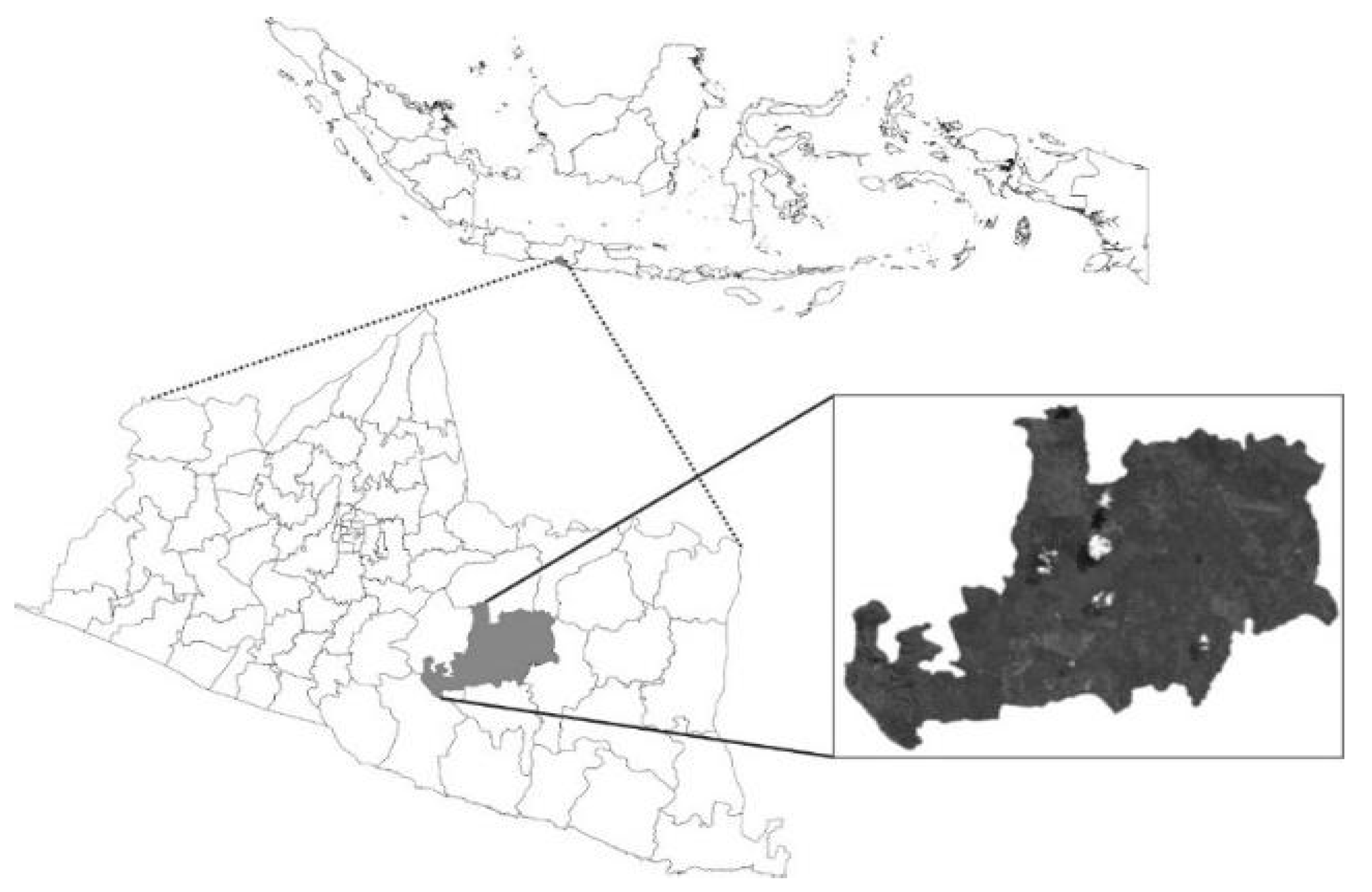
2.1. Study Site
2.2. Experimental Design and Crop Management
2.3. Data Collection
2.4. Statistical Analysis
2.4.1. Selection of Candidate Models
2.4.2. Measures for Goodness-of-Fit
2.4.3. Evaluation of Model Assumptions
2.4.4. Model Calibration
2.4.5. Data Analysis
3. Results
3.1. Choose Candidate Models for Determining CPWC
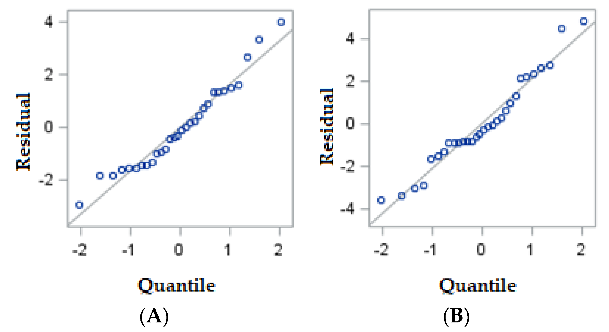
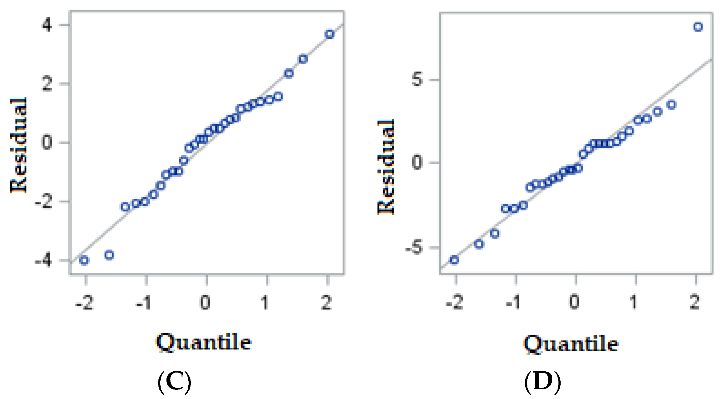
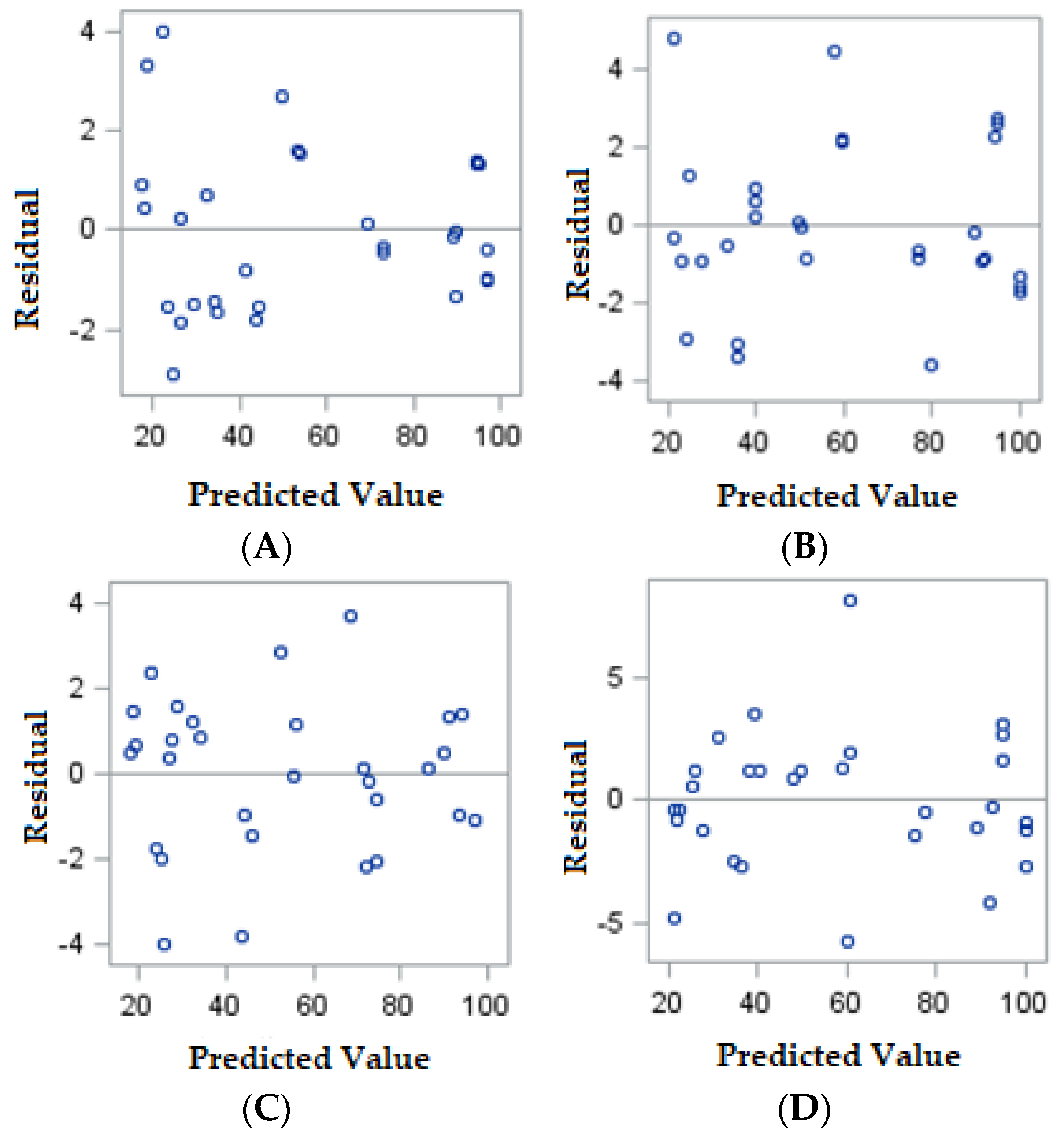
3.2. Evaluation of Model Assumptions
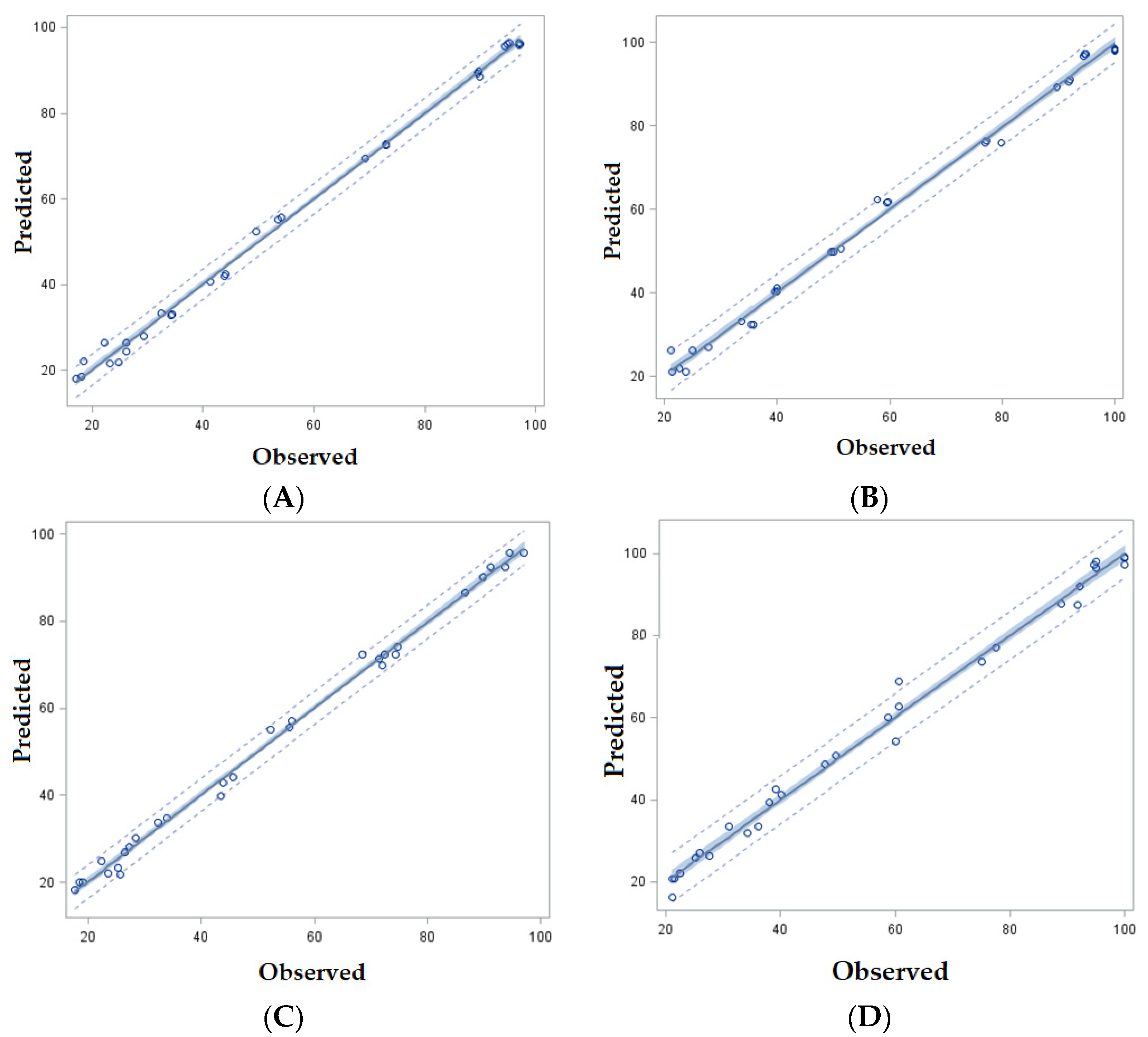
3.3. Model Calibration
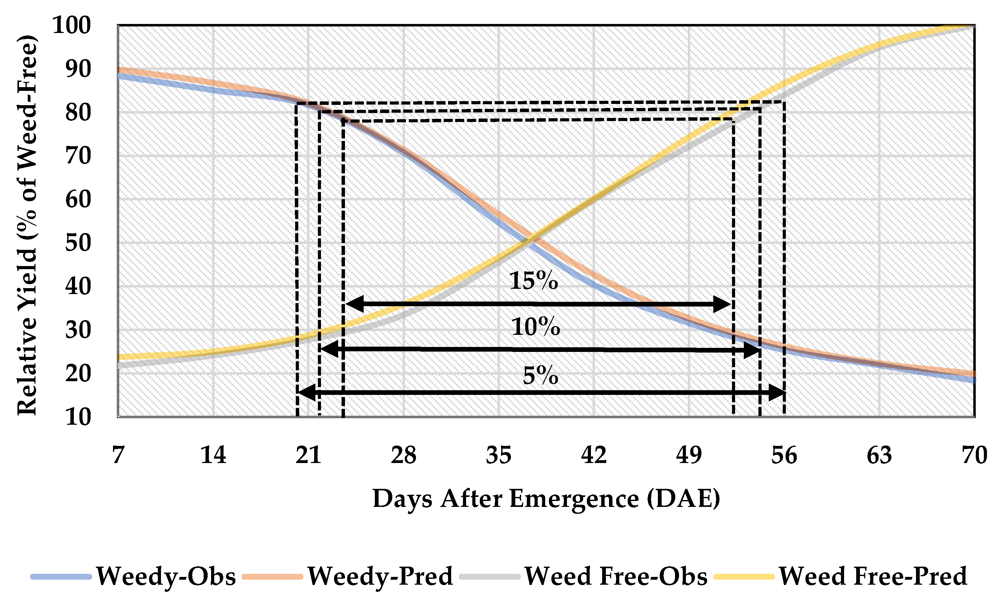
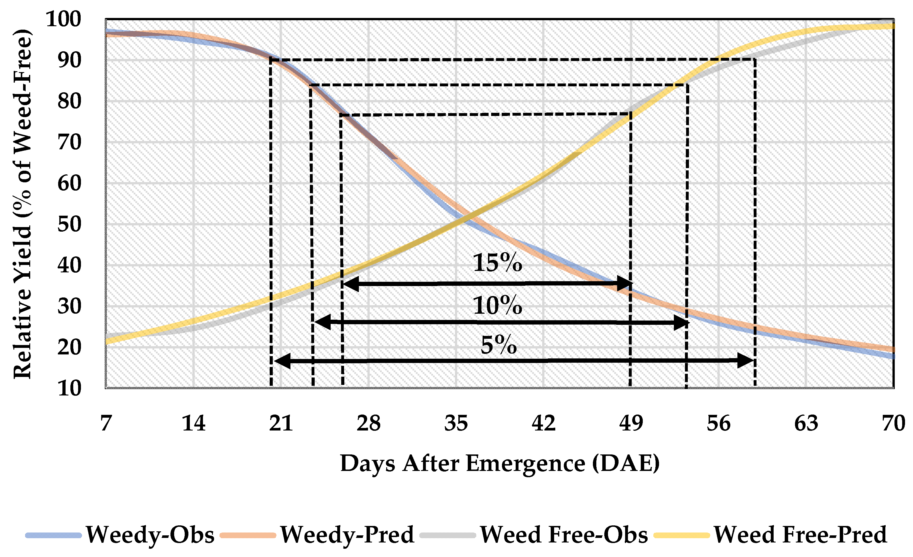
3.4. Predicted AYL Based on the Best Fitted Model
4. Discussion
5. Conclusions
Author Contributions
Funding
Institutional Review Board Statement
Informed Consent Statement
Data Availability Statement
Acknowledgments
Conflicts of Interest
References
- Abbas, A.; Khaliq, A.; Saqib, M.; Majeed, M.Z.; Ullah, S.; Haroon, M. Influence of tillage systems and selective herbicides on weed management and productivity of direct-seeded rice (Oryza sativa). Planta Daninha 2019, 37, 1–15. [Google Scholar] [CrossRef]
- Hosseini, S.Z.; Firouzi, S.; Aminpanah, H.; Sadeghnejhad, H.R. Effect of tillage system on yield and weed populations of soybean (Glycine max L.). An. Acad. Bras. Ciências 2016, 88, 377–384. [Google Scholar] [CrossRef] [PubMed] [Green Version]
- Swanton, C.J.; O’Sullivan, J.; Robinson, D.E. The critical weed-free period in carrot. Weed Sci. 2010, 58, 229–233. [Google Scholar] [CrossRef]
- Travlos, I.S.; Cheimona, N.; Roussis, I.; Bilalis, D.J. Weed-species abundance and diversity indices in relation to tillage systems and fertilization. Front. Environ. Sci. 2018, 6, 11. [Google Scholar] [CrossRef] [Green Version]
- Bastiaans, L.; Kropff, M.J. Weed competition. In Encyclopedia of Applied Plant Sciences: Crop Systems, 2nd ed.; Thomas, B., Murray, B.G., Murphy, D.J., Eds.; Academic Press: New York, NY, USA, 2017; Volume 3, pp. 473–478. [Google Scholar]
- McLeod, R. Annual Costs of Weeds in Australia; eSYS Development Pty Limited: Sydney, NSW, Australia, 2018; pp. 9–14. [Google Scholar]
- Shrestha, A.; Thapa, B.; Devkota, M.; Subedi, R. Comparative efficiency of different weed management practices on yield and economic in summer maize in Dang. Adv. Crop. Sci. Tech. 2018, 6, 2. [Google Scholar]
- Suryanto, P.; Tohari, S.E.; Putra, E.T.S.; Kastono, D.; Alam, T. Estimation of critical period for weed control in soybean on agro-forestry system with kayu putih. Asian J. Crop Sci. 2017, 9, 82–91. [Google Scholar] [CrossRef]
- Knezevic, S.Z.; Datta, A. The critical period for weed control: Revisiting data analysis. Weed Sci. 2015, 63, 188–202. [Google Scholar] [CrossRef] [Green Version]
- Zandoná, R.R.; Agostinetto, D.; Silva, B.M.; Ruchel, Q.; Fraga, D.S. Interference periods in soybean crop as affected by emergence times of weeds. Planta Daninha 2018, 36, e018169361. [Google Scholar] [CrossRef] [Green Version]
- Hartzler, R. Is Your Weed Management Program Reducing Your Economic Return? Iowa State University: Ames, IA, USA, 2003; Available online: http://extension.agron.iastate.edu/weeds/mgmt/2003/economics.shtml (accessed on 9 February 2022).
- Knezevic, S.Z.; Evans, S.P.; Blankenship, E.E.; Van Acker, R.C.; Lindquist, J.L. Critical period of weed control: The concept and data analysis. Weed Sci. 2002, 50, 773–786. [Google Scholar] [CrossRef] [Green Version]
- Hendrival, W.; Zurrahmi; Abdul, A. Critical period for weed control competition in soybean. Floratek J. 2014, 9, 6–13. [Google Scholar]
- Archontoulisa, S.V.; Miguez, F.E. Nonlinear regression models and applications in agricultural research. Agron. J. 2014, 107, 786–798. [Google Scholar] [CrossRef] [Green Version]
- Cardoso, G.D.; Alves, P.L.C.A.; Severino, L.S.; Vale, L.S. Critical periods of weed control in naturally green colored cotton BRS Verde. Ind. Crops Prod. 2011, 34, 1198–1202. [Google Scholar] [CrossRef]
- Singh, M.; Bhullar, M.S.; Chauhan, B.S. The critical period for weed control in dry-seeded rice. Crop Prot. 2011, 66, 80–85. [Google Scholar] [CrossRef]
- Singh, M.; Bhullar, M.S.; Chauhan, B.S. Relative time of weed and crop emergence is crucial for managing weed seed production: A study under an aerobic rice system. Crop Prot. 2017, 99, 33–38. [Google Scholar] [CrossRef]
- Stagnari, F.; Pisante, M. The critical period for weed competition in French bean (Phaseolus vulgaris L.) in Mediterranean areas. Crop Prot. 2011, 30, 179–184. [Google Scholar] [CrossRef]
- Seyyedi, S.M.; Moghaddam, P.R.; Mahallati, M.N. Weed competition periods affect grain yield and nutrient uptake of black seed (Nigella Sativa L.). Hortic. Plant J. 2016, 2, 172–180. [Google Scholar] [CrossRef] [Green Version]
- Tursun, N.; Datta, A.; Tuncel, E.; Kantarci, Z.; Knezevic, S.Z. Nitrogen application influenced the critical period for weed control in cotton. Crop Prot. 2015, 74, 85–91. [Google Scholar] [CrossRef]
- Tursun, N.; Datta, A.; Sakinmaz, M.S.; Kantarci, Z.; Knezevic, S.Z.; Chauhan, B.S. The critical period for weed control in three corn (Zea mays L.) types. Crop Prot. 2016, 90, 59–65. [Google Scholar] [CrossRef]
- Alam, T.; Kurniasih, B.; Suryanto, P.; Basunanda, P.; Supriyanta; Ambarwati, E.; Widyawan, M.H.; Handayani, S.; Taryono. Stability analysis for soybean in agroforestry system with kayu putih. SABRAO J. Breed. Genet. 2019, 51, 405–418. [Google Scholar]
- Alam, T.; Suryanto, P.; Handayani, S.; Kastono, D.; Kurniasih, B. Optimizing application of biochar, compost and nitrogen fertilizer in soybean intercropping with kayu putih (Melaleuca cajuputi). Rev. Bras. Cienc. Solo 2020, 44, 1–17. [Google Scholar] [CrossRef]
- Kuri-Morales, A.; Rodríguez-Erazo, F. A search space reduction methodology for large databases: A case study. In Advances in Data Mining: Theoretical Aspects and Applications; Carbonell, J.G., Siekmann, J., Eds.; Springer: Leipzig, Germany, 2007; pp. 204–205. [Google Scholar]
- Satter, A.; Iqbal, G.M. Decline curve analysis for conventional and unconventional reservoirs. Reservoir. Eng. 2016, 211–232. Available online: https://www.researchgate.net/publication/314643400_Decline_curve_analysis_for_conventional_and_unconventional_reservoirs (accessed on 20 June 2022).
- Ritz, C.; Baty, F.; Streibig, J.C.; Gerhard, D. Dose-response analysis using R. PLoS ONE 2015, 10, e0146021. [Google Scholar]
- Hyams, D.G. CurveExpert Professional Documentation. Available online: https://www.curveexpert.net/docs/curveexpert/pro/pdf/CurveExpertProfessional.pdf (accessed on 9 February 2022).
- Ratkowsky, D.A. Handbook of Nonlinear Regression Models; Marcel Dekker: New York, NY, USA, 1990; pp. 123–147. [Google Scholar]
- Richards, F.J. The quantitative analysis of growth. In Plant Physiology; Steward, F.C., Ed.; Academic Press: New York, NY, USA, 1969; pp. 3–76. [Google Scholar]
- Weibull, W. A statistical distribution function of wide applicability. J. Appl. Mech. 1951, 18, 293–297. [Google Scholar] [CrossRef]
- Wallach, D. Evaluating crop models. In Working with Dynamic Crop Models: Evaluations, Analysis, Parameterization, and Applications, 1st ed.; Wallach, D., Makowski, D., Jones, J., Eds.; Elsevier: Amsterdam, The Netherlands, 2006; pp. 11–53. [Google Scholar]
- Anderson-Sprecher, R. Model comparisons and R-square. Am. Stat. 1994, 48, 113–117. [Google Scholar]
- Kvalseth, T.O. Cautionary note about R2. Am. Stat. 1985, 39, 279–285. [Google Scholar]
- Burnham, K.P.; Anderson, D.R. Model Selection and Inference: A Practical Information-Theoretic Approach, 2nd ed.; Springer: New York, NY, USA, 2003; pp. 271–273. [Google Scholar]
- Akaike, H. A new look at the statistical model identification. IEEE Trans. Autom. Control. 1974, 19, 716–723. [Google Scholar] [CrossRef]
- Schwarz, G. Estimating the dimension of a model. Ann. Stat. 1978, 6, 461–464. [Google Scholar] [CrossRef]
- Ritz, C.; Streibig, J.C. Nonlinear Regression with R; Springer: New York, NY, USA, 2008; pp. 4–6. [Google Scholar]
- Bhattacharyya, M. To pool or not to pool: A comparison between two commonly used test statistics. Int. J. Pure Appl. Math. 2013, 89, 497–510. [Google Scholar] [CrossRef] [Green Version]
- SAS Institute Inc. Step-by-Step Programming with Base SAS® 9.4, 2nd ed.; SAS Institute Inc.: Cary, NC, USA, 2013. [Google Scholar]
- Baty, F.; Ritz, C.; Charles, S.; Brutsche, M.; Flandrois, J.P.; Delignette-Muller, M.L. A toolbox for nonlinear regression in R: The package nlstools. J. Stat. Softw. 2015, 66, 1–21. [Google Scholar] [CrossRef] [Green Version]
- Lewis, F.; Butler, A.; Gilbert, L. A unified approach to model selection using the likelihood ratio test. Methods Ecol. Evol. 2011, 2, 155–162. [Google Scholar] [CrossRef]
- Spiess, A.N.; Neumeyer, N. An evaluation of R2 as an inadequate measure for nonlinear models in pharmacological and biochemical research: A Monte Carlo approach. BMC Pharmacol. 2010, 10, 6. [Google Scholar] [CrossRef] [Green Version]
- Draper, N.R.; Smith, H. Applied Regression Analysis, 3rd ed.; John Wiley & Sons, Inc.: New York, NY, USA, 1998; pp. 243–250. [Google Scholar]
- Bauldry, S. Structural equation modeling. In International Encyclopedia of the Social & Behavioral Sciences, 2nd ed.; Wright, J.D., Ed.; Elsevier: Amsterdam, The Netherlands, 2015; pp. 615–620. [Google Scholar]
- Miguez, F.E.; Villamil, M.B.; Long, S.P.; Bollero, G.A. Meta-analysis of the effects of management factors on Miscanthus × giganteus growth and biomass production. Agric. For. Meteorol. 2008, 148, 1280–1292. [Google Scholar] [CrossRef]
- Amaducci, S.; Colauzzi, M.; Bellocchi, G.; Venturi, G. Modelling post-emergent hemp phenology (Cannabis sativa L.): Theory and evaluation. Eur J. Agron. 2008, 28, 90–102. [Google Scholar] [CrossRef]
- Dagogo, J.; Nduka, E.C.; Ogoke, U.P. Comparative analysis of richards, gompertz and weibull models. IOSR J. Math. 2020, 16, 15–25. [Google Scholar]
- Mahanta, D.J.; Borah, M. Parameter estimation of weibull growth models in forestry. Int. J. Math. Trends Technol. 2014, 8, 158–163. [Google Scholar]
- Colff, M.V.D.; Kimberley, M.O. A national height-age model for Pinus radiata in New Zealand. N. Z. J. For. Sci. 2013, 43, 1–11. [Google Scholar]
- Sholikin, M.M.; Alifian, M.D.; Purba, F.M.; Harahap, R.P.; Jayanegara, A.; Nahrowi. Evaluate Non-Linear Model Logistic, Gompertz, and Weibull: Study Case on Calcium and Phosphor Requirements of Laying Hen. In Proceedings of the Conference Series: Earth and Environmental Science, Malang, Indonesia, 24–27 October 2020. [Google Scholar]
- Raji, A.O.; Mbap, S.T.; Aliyu, J. Comparison of different models to describe growth of the japanese quail (Coturnix japonica). Trakia J. Sci. 2014, 12, 182–188. [Google Scholar]
- Svagelj, W.S.; Laich, A.G.; Quintana, F. Richards’s equation and nonlinear mixed models applied to avian growth: Why use them? J. Avian Biol. 2019, 2019, 1–8. [Google Scholar] [CrossRef] [Green Version]
- Teleken, J.T.; Galvão, A.C.; Robazza, W.S. Use of modified Richards model to predict isothermal and non-isothermal microbial growth. Braz. J. Microbiol. 2018, 49, 614–620. [Google Scholar] [CrossRef]
- Ritz, P.P.; Rogers, M.B.; Zabinsky, J.S.; Hedrick, V.E.; Rockwell, J.A.; Rimer, E.G. Dietary and biological assessment of the omega-3 status of collegiate athletes: A cross-sectional analysis. PLoS ONE 2020, 15, e0228834. [Google Scholar] [CrossRef]
- Gesztelyi, R.; Zsuga, J.; Kemeny-Beke, A.; Varga, B.; Juhasz, B.; Tosaki, A. The hill equation and the origin of quantitative pharmacology. Arch. Hist. Exact Sci. 2012, 66, 427–438. [Google Scholar] [CrossRef]
- Sobko, O.; Stahl, A.; Hahn, V.; Zikeli, S.; Claupein, W.; Gruber, S. Environmental effects on soybean (Glycine max (L.) Merr) production in Central and South Germany. Agronomy 2020, 10, 1847. [Google Scholar] [CrossRef]


| Duration of Weedy and Weed-Free Periods 1 | Remarks |
|---|---|
| W—0 DAE | Weedy until 70 days after emergence (DAE) |
| W—7 DAE | Weedy after 7 until 70 DAE |
| W—14 DAE | Weedy after 14 until 70 DAE |
| W—21 DAE | Weedy after 21 until 70 DAE |
| W—28 DAE | Weedy after 28 until 70 DAE |
| W—35 DAE | Weedy after 35 until 70 DAE |
| W—42 DAE | Weedy after 42 until 70 DAE |
| W—49 DAE | Weedy after 49 until 70 DAE |
| W—56 DAE | Weedy after 56 until 70 DAE |
| W—63 DAE | Weedy after 63 until 70 DAE |
| WF—7 DAE | Weed-Free after 7 until 70 DAE |
| WF—14 DAE | Weed-Free after 14 until 70 DAE |
| WF—21 DAE | Weed-Free after 21 until 70 DAE |
| WF—28 DAE | Weed-Free after 28 until 70 DAE |
| WF—35 DAE | Weed-Free after 35 until 70 DAE |
| WF—42 DAE | Weed-Free after 42 until 70 DAE |
| WF—49 DAE | Weed-Free after 49 until 70 DAE |
| WF—56 DAE | Weed-Free after 56 until 70 DAE |
| WF—63 DAE | Weed-Free after 63 until 70 DAE |
| WF—0 DAE | Weed-Free until 70 DAE |
| Decline | Distribution | Dose–Response | Exponential | Growth | Miscellaneous | Power Law Family | Sigmoidal | Yield-Spacing Models |
|---|---|---|---|---|---|---|---|---|
|
|
|
|
|
|
|
|
|
|
|
|
|
|
|
|
|
|
|
|
|
|
|
|
|
|
|
|
|
|
|
|
|
| ||
|
|
|
|
| ||||
|
|
| ||||||
|
| |||||||
|
| No. | Model | Family | Equation | References |
|---|---|---|---|---|
| 1. | Bleasdale | Yield-Spacing Models | [24] | |
| 2. | Exponential | Exponential Models | [24] | |
| 3. | Exponential Association 2 | Growth Models | [24] | |
| 4. | Exponential Association 3 | Growth Models | [24] | |
| 5. | Exponential Decline | Decline Models | [25] | |
| 6. | Farazdaghi–Harris | Yield-Spacing Models | [26] | |
| 7. | DR-Gamma | Dose–Response Models | [26] | |
| 8. | DR-Hill | Dose–Response Models | [26] | |
| 9. | DR-Logistic | Dose–Response Models | [26] | |
| 10. | DR-Probit | Dose–Response Models | [26] | |
| 11. | DR-Weibull | Dose–Response Models | [26] | |
| 12. | Gaussian Model | Miscellaneous | [24] | |
| 13. | Geometric | Power Law Family | [24] | |
| 14. | Gompertz Relation | Sigmoidal Models | [24] | |
| 15. | Harmonic Decline | Decline Models | [24] | |
| 16. | Hyperbolic Decline | Decline Models | [24] | |
| 17. | Heat Capacity | Miscellaneous | [24] | |
| 18. | Hoerl | Power Law Family | [27] | |
| 19. | Logistic | Sigmoidal Models | [24] | |
| 20. | Logistic Power | Sigmoidal Models | [27] | |
| 21. | Log Normal CDF | Distribution Models | [27] | |
| 22. | Log Normal PDF | Distribution Models | [27] | |
| 23. | Modified Exponential | Exponential Models | [24] | |
| 24. | Modified Geometric | Power Law Family | [24] | |
| 25. | Modified Hoerl | Power Law Family | [24] | |
| 26. | Modified Power | Power Law Family | [24] | |
| 27. | Morgan–Mercer–Flodin (MMF) | Sigmoidal Models | [28] | |
| 28. | Natural Logarithm | Exponential Models | [27] | |
| 29. | Normal (Gaussian) CDF | Distribution Models | [27] | |
| 30. | Normal (Gaussian) PDF | Distribution Models | [27] | |
| 31. | Power | Power Law Family | [24] | |
| 32. | Rational Model | Miscellaneous | [24] | |
| 33. | Ratkowsky | Sigmoidal Models | [28] | |
| 34. | Reciprocal | Yield-Spacing Models | [24] | |
| 35. | Reciprocal Logarithm | Exponential Models | [27] | |
| 36. | Reciprocal Quadratic | Yield-Spacing Models | [24] | |
| 37. | Richards | Sigmoidal Models | [29] | |
| 38. | Root | Power Law Family | [24] | |
| 39. | Saturation Growth Rate | Growth Models | [24] | |
| 40. | Shifted Power | Power Law Family | [24] | |
| 41. | Sinusoidal | Miscellaneous | [24] | |
| 42. | Steinhart–Hart Equation | Miscellaneous | [24] | |
| 43. | Truncated Fourier Series | Miscellaneous | [27] | |
| 44. | Vapour Pressure Model | Exponential Models | [24] | |
| 45. | Weibull | Sigmoidal Models | [30] |
| No. | Models | Periods 1 | Goodness-of-Fit | |||
|---|---|---|---|---|---|---|
| RMSE | AICc | BIC | ||||
| 1. | Bleasdale | W | 0.946 | 8.143 | 44.091 | 52.018 |
| WF | 0.952 | 7.348 | 42.035 | 49.529 | ||
| 2. | Exponential | W | 0.933 | 7.607 | 40.851 | 48.092 |
| WF | 0.952 | 6.873 | 38.819 | 45.628 | ||
| 3. | Exponential Association 2 | W | 0.000 | 32.789 | 70.070 | 83.550 |
| WF | 0.966 | 5.796 | 35.411 | 41.523 | ||
| 4. | Exponential Association 3 | W | 0.956 | 7.340 | 42.015 | 49.500 |
| WF | 0.974 | 5.397 | 35.863 | 42.065 | ||
| 5. | Exponential Decline | W | 0.946 | 7.617 | 40.876 | 48.122 |
| WF | 0.952 | 6.873 | 38.819 | 45.628 | ||
| 6. | Farazdaghi–Harris | W | 0.991 | 3.246 | 25.697 | 30.163 |
| WF | 0.957 | 6.951 | 40.925 | 48.180 | ||
| 7. | DR-Gamma | W | 0.986 | 4.099 | 30.361 | 35.585 |
| WF | 0.000 | 33.528 | 72.395 | 86.167 | ||
| 8. | DR-Hill | W | 0.000 | 37.861 | 77.570 | 92.334 |
| WF | 0.991 | 3.490 | 29.890 | 34.974 | ||
| 9. | DR-Logistic | W | 0.000 | 73.558 | 88.109 | 104.131 |
| WF | 0.000 | 77.572 | 89.172 | 105.216 | ||
| 10. | DR-Probit | W | 0.000 | 73.558 | 88.109 | 104.131 |
| WF | 0.000 | 77.572 | 89.172 | 105.216 | ||
| 11. | DR-Weibull | W | 0.000 | 73.558 | 88.109 | 104.131 |
| WF | 0.000 | 77.572 | 89.172 | 105.216 | ||
| 12. | Gaussian | W | 0.983 | 4.125 | 30.487 | 35.733 |
| WF | 0.987 | 3.813 | 28.913 | 33.832 | ||
| 13. | Geometric | W | 0.967 | 5.973 | 36.015 | 42.280 |
| WF | 0.936 | 7.949 | 41.731 | 49.159 | ||
| 14. | Gompertz Relation | W | 0.000 | 31.328 | 71.038 | 84.698 |
| WF | 0.983 | 4.427 | 31.902 | 37.343 | ||
| 15. | Harmonic Decline | W | 0.859 | 12.326 | 50.503 | 59.836 |
| WF | 0.872 | 11.199 | 48.585 | 57.518 | ||
| 16. | Hyperbolic Decline | W | 0.969 | 6.192 | 38.613 | 45.394 |
| WF | 0.978 | 4.925 | 34.032 | 39.874 | ||
| 17. | Heat Capacity | W | 0.957 | 7.270 | 41.822 | 49.266 |
| WF | 0.984 | 4.334 | 31.477 | 36.841 | ||
| 18. | Hoerl | W | 0.990 | 3.101 | 24.783 | 29.113 |
| WF | 0.973 | 5.483 | 36.181 | 42.447 | ||
| 19. | Logistic | W | 0.843 | 12.427 | 52.545 | 62.331 |
| WF | 0.987 | 3.829 | 28.999 | 33.932 | ||
| 20. | Logistic Power | W | 0.992 | 2.710 | 22.085 | 26.039 |
| WF | 0.968 | 5.973 | 37.890 | 44.505 | ||
| 21. | Log Normal CDF | W | 0.000 | 68.807 | 84.895 | 100.613 |
| WF | 0.000 | 72.642 | 85.979 | 101.690 | ||
| 22. | Log Normal PDF | W | 0.000 | 64.208 | 83.573 | 99.144 |
| WF | 0.000 | 66.136 | 84.103 | 99.595 | ||
| 23. | Modified Exponential | W | 0.512 | 22.901 | 62.891 | 74.936 |
| WF | 0.888 | 10.521 | 47.336 | 55.992 | ||
| 24. | Modified Geometric | W | 0.640 | 19.688 | 59.869 | 71.269 |
| WF | 0.931 | 8.268 | 42.515 | 50.113 | ||
| 25. | Modified Hoerl | W | 0.972 | 5.903 | 37.657 | 44.246 |
| WF | 0.982 | 4.560 | 32.493 | 38.043 | ||
| 26. | Modified Power | W | 0.946 | 7.617 | 40.876 | 48.122 |
| WF | 0.952 | 6.873 | 38.819 | 45.628 | ||
| 27. | MMF | W | 0.996 | 2.097 | 19.414 | 23.035 |
| WF | 0.980 | 4.721 | 33.189 | 38.870 | ||
| 28. | Natural Logarithm | W | 0.863 | 10.852 | 47.956 | 56.725 |
| WF | 0.832 | 12.840 | 51.320 | 60.857 | ||
| 29. | Normal (Gaussian) CDF | W | 0.000 | 68.807 | 84.895 | 100.613 |
| WF | 0.000 | 72.701 | 85.996 | 101.709 | ||
| 30. | Normal (Gaussian) PDF | W | 0.000 | 61.212 | 82.556 | 98.006 |
| WF | 0.000 | 65.515 | 83.914 | 99.383 | ||
| 31. | Power | W | 0.731 | 15.178 | 54.666 | 64.924 |
| WF | 0.968 | 5.586 | 34.675 | 40.642 | ||
| 32. | Rational Model | W | 0.996 | 2.323 | 21.748 | 25.658 |
| WF | 0.995 | 2.608 | 24.065 | 28.268 | ||
| 33. | Ratkowsky | W | 0.982 | 4.223 | 30.962 | 36.291 |
| WF | 0.987 | 3.829 | 28.999 | 33.932 | ||
| 34. | Reciprocal | W | 0.859 | 50.503 | 50.503 | 59.836 |
| WF | 0.873 | 11.199 | 48.586 | 57.519 | ||
| 35. | Reciprocal Logarithm | W | 0.641 | 19.634 | 59.814 | 71.202 |
| WF | 0.958 | 6.449 | 37.547 | 44.092 | ||
| 36. | Reciprocal Quadratic | W | 0.996 | 2.311 | 18.904 | 22.466 |
| WF | 0.995 | 2.435 | 21.532 | 25.443 | ||
| 37. | Richards | W | 0.995 | 2.379 | 22.222 | 26.194 |
| WF | 0.996 | 2.298 | 19.944 | 23.708 | ||
| 38. | Root | W | 0.512 | 22.901 | 62.892 | 74.937 |
| WF | 0.888 | 10.521 | 47.336 | 55.992 | ||
| 39. | Saturation Growth Rate | W | 0.438 | 24.580 | 64.308 | 76.648 |
| WF | 0.966 | 5.794 | 35.405 | 41.516 | ||
| 40. | Shifted Power | W | 0.918 | 10.010 | 48.219 | 57.046 |
| WF | 0.978 | 4.925 | 34.032 | 39.874 | ||
| 41. | Sinusoidal | W | 0.994 | 2.694 | 24.711 | 29.031 |
| WF | 0.992 | 3.191 | 28.099 | 32.885 | ||
| 42. | Steinhart–Hart Equation | W | 0.957 | 7.236 | 41.729 | 49.154 |
| WF | 0.980 | 4.721 | 33.189 | 38.870 | ||
| 43. | Truncated Fourier Series | W | 0.000 | 73.623 | 90.870 | 107.092 |
| WF | 0.000 | 79.345 | 92.368 | 108.695 | ||
| 44. | Vapour Pressure Model | W | 0.954 | 6.726 | 40.266 | 47.386 |
| WF | 0.981 | 4.560 | 32.493 | 38.043 | ||
| 45. | Weibull | W | 0.997 | 1.732 | 15.883 | 19.128 |
| WF | 0.993 | 3.113 | 27.601 | 32.308 | ||
| No. | Models | Periods 1 | Goodness-of-Fit | |||
|---|---|---|---|---|---|---|
| RMSE | AICc | BIC | ||||
| 1. | Bleasdale | W | 0.931 | 8.188 | 44.200 | 52.151 |
| WF | 0.961 | 6.741 | 40.311 | 47.435 | ||
| 2. | Exponential | W | 0.947 | 7.533 | 40.653 | 47.853 |
| WF | 0.961 | 6.305 | 37.095 | 43.547 | ||
| 3. | Exponential Association 2 | W | 0.000 | 29.249 | 67.786 | 80.828 |
| WF | 0.966 | 5.858 | 35.625 | 41.780 | ||
| 4. | Exponential Association 3 | W | 0.961 | 6.183 | 38.585 | 45.361 |
| WF | 0.969 | 5.970 | 37.882 | 44.496 | ||
| 5. | Exponential Decline | W | 0.931 | 7.659 | 40.985 | 48.254 |
| WF | 0.961 | 6.305 | 37.095 | 43.547 | ||
| 6. | Farazdaghi–Harris | W | 0.992 | 2.861 | 23.171 | 27.272 |
| WF | 0.960 | 6.796 | 40.475 | 47.634 | ||
| 7. | DR-Gamma | W | 0.987 | 3.526 | 27.351 | 32.074 |
| WF | 0.000 | 34.020 | 72.687 | 86.509 | ||
| 8. | DR-Hill | W | 0.997 | 1.822 | 16.893 | 20.238 |
| WF | 0.993 | 3.115 | 27.618 | 32.328 | ||
| 9. | DR-Logistic | W | 0.000 | 69.330 | 86.925 | 102.844 |
| WF | 0.000 | 75.296 | 88.576 | 104.562 | ||
| 10. | DR-Probit | W | 0.000 | 69.330 | 86.925 | 102.844 |
| WF | 0.000 | 75.296 | 88.576 | 104.562 | ||
| 11. | DR-Weibull | W | 0.000 | 69.330 | 86.925 | 102.844 |
| WF | 0.000 | 75.296 | 88.576 | 104.562 | ||
| 12. | Gaussian | W | 0.981 | 4.790 | 33.478 | 39.261 |
| WF | 0.987 | 29.496 | 29.496 | 34.513 | ||
| 13. | Geometric | W | 0.956 | 6.119 | 36.498 | 42.858 |
| WF | 0.947 | 7.319 | 40.079 | 47.154 | ||
| 14. | Gompertz Relation | W | 0.000 | 35.125 | 73.326 | 87.396 |
| WF | 0.983 | 4.423 | 31.885 | 37.323 | ||
| 15. | Harmonic Decline | W | 0.842 | 11.615 | 49.314 | 58.383 |
| WF | 0.883 | 10.894 | 48.033 | 56.844 | ||
| 16. | Hyperbolic Decline | W | 0.965 | 5.845 | 37.458 | 44.007 |
| WF | 0.980 | 4.810 | 33.563 | 39.315 | ||
| 17. | Heat Capacity | W | 0.965 | 5.861 | 37.515 | 44.076 |
| WF | 0.983 | 4.384 | 31.705 | 37.110 | ||
| 18. | Hoerl | W | 0.992 | 3.116 | 24.877 | 29.221 |
| WF | 0.975 | 5.403 | 35.888 | 42.095 | ||
| 19. | Logistic | W | 0.859 | 13.186 | 53.731 | 63.781 |
| WF | 0.961 | 6.740 | 40.309 | 47.433 | ||
| 20. | Logistic Power | W | 0.992 | 3.037 | 24.363 | 28.632 |
| WF | 0.966 | 6.242 | 38.772 | 45.571 | ||
| 21. | Log Normal CDF | W | 0.000 | 64.852 | 83.711 | 99.298 |
| WF | 0.000 | 70.469 | 85.372 | 101.014 | ||
| 22. | Log Normal PDF | W | 0.000 | 58.588 | 81.680 | 97.021 |
| WF | 0.000 | 63.230 | 83.204 | 98.586 | ||
| 23. | Modified Exponential | W | 0.884 | 10.860 | 47.971 | 56.744 |
| WF | 0.888 | 10.661 | 47.600 | 56.315 | ||
| 24. | Modified Geometric | W | 0.608 | 18.314 | 58.421 | 69.506 |
| WF | 0.927 | 8.618 | 43.346 | 51.125 | ||
| 25. | Modified Hoerl | W | 0.952 | 6.845 | 40.618 | 47.811 |
| WF | 0.983 | 4.379 | 31.684 | 37.085 | ||
| 26. | Modified Power | W | 0.931 | 7.659 | 40.985 | 48.254 |
| WF | 0.961 | 6.305 | 37.095 | 43.547 | ||
| 27. | MMF | W | 0.996 | 2.296 | 21.519 | 25.399 |
| WF | 0.978 | 5.410 | 38.656 | 45.431 | ||
| 28. | Natural Logarithm | W | 0.892 | 10.797 | 47.854 | 56.601 |
| WF | 0.808 | 13.928 | 52.947 | 62.841 | ||
| 29. | Normal (Gaussian) CDF | W | 0.000 | 64.852 | 83.711 | 99.298 |
| WF | 0.000 | 70.567 | 85.400 | 101.045 | ||
| 30. | Normal (Gaussian) PDF | W | 0.000 | 58.407 | 81.617 | 96.950 |
| WF | 0.000 | 65.701 | 83.971 | 99.447 | ||
| 31. | Power | W | 0.760 | 16.086 | 55.827 | 66.342 |
| WF | 0.966 | 5.838 | 35.558 | 41.699 | ||
| 32. | Rational Model | W | 0.996 | 2.453 | 22.839 | 26.894 |
| WF | 0.996 | 2.323 | 21.748 | 25.681 | ||
| 33. | Ratkowsky | W | 0.982 | 4.725 | 33.205 | 38.938 |
| WF | 0.987 | 3.824 | 28.973 | 33.902 | ||
| 34. | Reciprocal | W | 0.842 | 11.615 | 49.314 | 58.383 |
| WF | 0.883 | 10.894 | 48.033 | 56.844 | ||
| 35. | Reciprocal Logarithm | W | 0.620 | 18.032 | 58.112 | 69.129 |
| WF | 0.961 | 6.304 | 37.091 | 43.542 | ||
| 36. | Reciprocal Quadratic | W | 0.993 | 2.573 | 21.051 | 24.871 |
| WF | 0.996 | 2.194 | 20.608 | 24.430 | ||
| 37. | Richards | W | 0.997 | 2.125 | 19.971 | 23.658 |
| WF | 0.996 | 2.194 | 17.464 | 21.061 | ||
| 38. | Root | W | 0.481 | 21.063 | 61.219 | 72.909 |
| WF | 0.888 | 10.661 | 47.600 | 56.315 | ||
| 39. | Saturation Growth Rate | W | 0.413 | 22.400 | 62.450 | 74.402 |
| WF | 0.966 | 5.847 | 35.597 | 41.746 | ||
| 40. | Shifted Power | W | 0.901 | 9.842 | 47.882 | 56.635 |
| WF | 0.980 | 4.810 | 33.563 | 39.315 | ||
| 41. | Sinusoidal | W | 0.989 | 3.960 | 32.415 | 38.003 |
| WF | 0.993 | 3.0819 | 27.403 | 32.080 | ||
| 42. | Steinhart–Hart Equation | W | 0.939 | 7.744 | 43.087 | 50.799 |
| WF | 0.980 | 4.774 | 33.411 | 39.134 | ||
| 43. | Truncated Fourier Series | W | 0.000 | 69.928 | 89.841 | 105.995 |
| WF | 0.000 | 76.577 | 91.658 | 107.926 | ||
| 44. | Vapour Pressure Model | W | 0.970 | 6.056 | 38.169 | 44.861 |
| WF | 0.983 | 4.379 | 31.682 | 37.083 | ||
| 45. | Weibull | W | 0.998 | 1.839 | 17.073 | 20.436 |
| WF | 0.994 | 0.9972 | 25.140 | 29.485 | ||
| AYL (%) | Dry Season | Wet Season | ||
|---|---|---|---|---|
| Beginning | End | Beginning | End | |
| 5 | 20 | 56 | 20 | 59 |
| 10 | 22 | 54 | 23 | 53 |
| 15 | 24 | 52 | 26 | 49 |
Publisher’s Note: MDPI stays neutral with regard to jurisdictional claims in published maps and institutional affiliations. |
© 2022 by the authors. Licensee MDPI, Basel, Switzerland. This article is an open access article distributed under the terms and conditions of the Creative Commons Attribution (CC BY) license (https://creativecommons.org/licenses/by/4.0/).
Share and Cite
Alam, T.; Suryanto, P.; Susyanto, N.; Kurniasih, B.; Basunanda, P.; Putra, E.T.S.; Kastono, D.; Respatie, D.W.; Widyawan, M.H.; Nurmansyah; et al. Performance of 45 Non-Linear Models for Determining Critical Period of Weed Control and Acceptable Yield Loss in Soybean Agroforestry Systems. Sustainability 2022, 14, 7636. https://doi.org/10.3390/su14137636
Alam T, Suryanto P, Susyanto N, Kurniasih B, Basunanda P, Putra ETS, Kastono D, Respatie DW, Widyawan MH, Nurmansyah, et al. Performance of 45 Non-Linear Models for Determining Critical Period of Weed Control and Acceptable Yield Loss in Soybean Agroforestry Systems. Sustainability. 2022; 14(13):7636. https://doi.org/10.3390/su14137636
Chicago/Turabian StyleAlam, Taufan, Priyono Suryanto, Nanang Susyanto, Budiastuti Kurniasih, Panjisakti Basunanda, Eka Tarwaca Susila Putra, Dody Kastono, Dyah Weny Respatie, Muhammad Habib Widyawan, Nurmansyah, and et al. 2022. "Performance of 45 Non-Linear Models for Determining Critical Period of Weed Control and Acceptable Yield Loss in Soybean Agroforestry Systems" Sustainability 14, no. 13: 7636. https://doi.org/10.3390/su14137636
APA StyleAlam, T., Suryanto, P., Susyanto, N., Kurniasih, B., Basunanda, P., Putra, E. T. S., Kastono, D., Respatie, D. W., Widyawan, M. H., Nurmansyah, Ansari, A., & Taryono. (2022). Performance of 45 Non-Linear Models for Determining Critical Period of Weed Control and Acceptable Yield Loss in Soybean Agroforestry Systems. Sustainability, 14(13), 7636. https://doi.org/10.3390/su14137636