
Pharmaceutical Supply Chain in China: Pricing and Production Decisions with Price-Sensitive and Uncertain Demand


Abstract
:1. Introduction
1.1. Motivations
- How can a mathematical model be developed to depict pricing and production decisions in China’s pharmaceutical supply chain with price-sensitive and uncertain demand?
- How do factors such as price sensitivity, ex-factory cost or governmental discounts influence the optimal decisions of drug retailers?
- Which factors have contributed to the drug shortage problem?
- Why do drugstores sometimes charge much more for a drug than hospitals do?
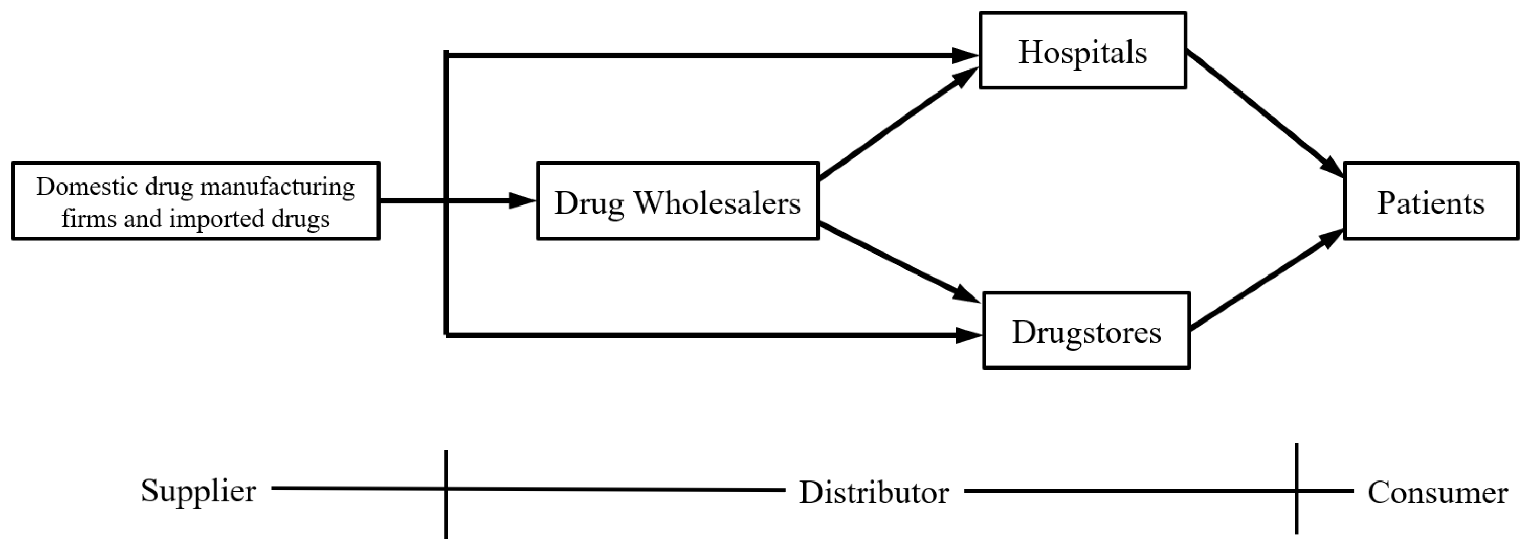
- Describing the drug pricing competition between drugstores and hospitals in China’s pharmaceutical supply chain.
- Obtaining the optimal strategies of participants in pharmaceutical supply chain and analyzing the influential factors of optimal prices, order quantities, profits and satisfaction rates.
- Identifying the main reasons for drug shortage and price disparity problems in China and providing suggestions for solving the problems.
1.2. Contributions
- Building a pricing model in China’s pharmaceutical supply chain with price-sensitive and uncertain demand considering governmental discount.
- Proving the existence and uniqueness of a pure-strategy Nash equilibrium in the game and deriving the closed form of two sellers’ optimal prices under the assumption of linear uniformly distributed demand.
- Analyzing the impacts of ex-factory price and government discounts on optimal prices and satisfaction rates to obtain insights on the drug shortage problem.
- Analyzing the impacts of price sensitivity on optimal prices, order quantities, expected profits, and satisfaction rates in two special cases of linear demand to provide insights into the price disparity problem.
- Providing suggestions for how the government can act to avoid drug shortage and price disparity problems.
2. Literature Review
2.1. Long-Term Decision Problems on Pharmaceutical Supply Chain
2.2. Short-Term Decision Problems on Pharmaceutical Supply Chain
2.3. Mid-Term Decision Problems on Pharmaceutical Supply Chain
2.4. Newvendor Problem with Different Approaches
2.5. Research Gap
3. Research Methods
3.1. Problem Description
3.2. Assumptions
- and are independent of and , furthermore, . So , .
- and are uniformly distributed on and respectively, where and .
- is twice continuous differentiable in on , so is in on .
- , .
- , .
- , and .
- and are increasing with and , respectively. i.e., and .
- and are non-increasing with and respectively, i.e., and .
- The linear form:where , , , , , are all positive.
- The logarithmic form:where , , , are all positive.
4. Model Formulation and Analysis
4.1. The Optimal Order Quantities of Hospital and Drugstore
4.2. Equilibrium Analysis
4.2.1. Existence of Nash Equilibrium
4.2.2. Uniqueness of Nash Equilibrium
4.3. Pricing Analysis with Linear Demand Functions
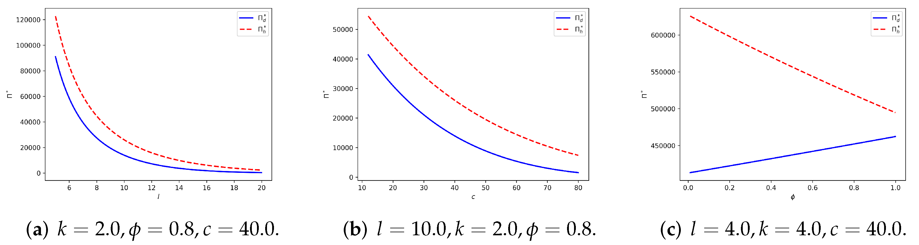
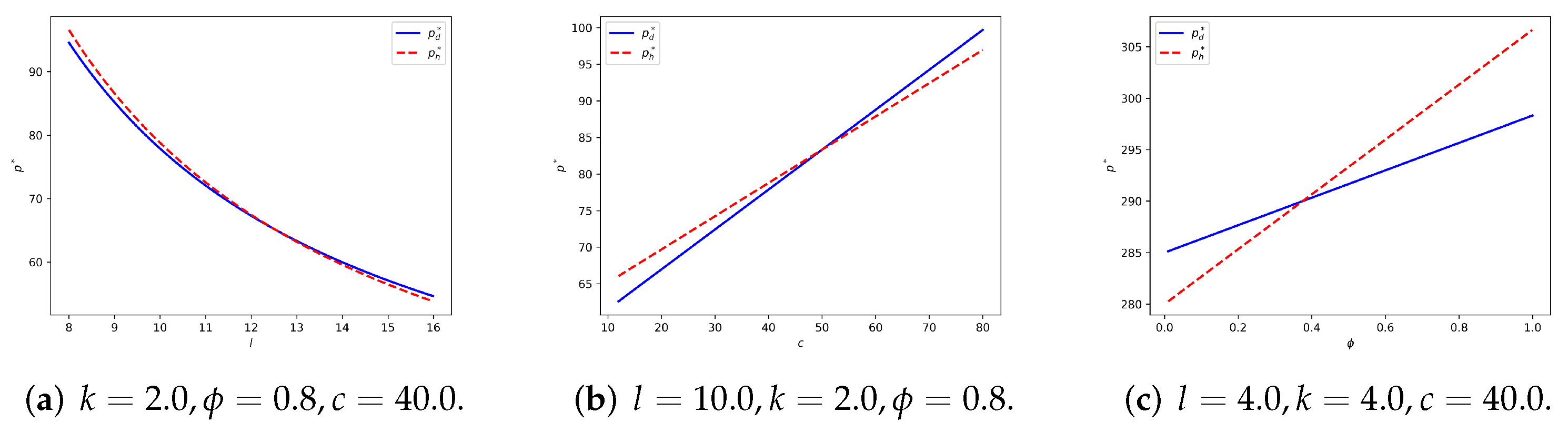
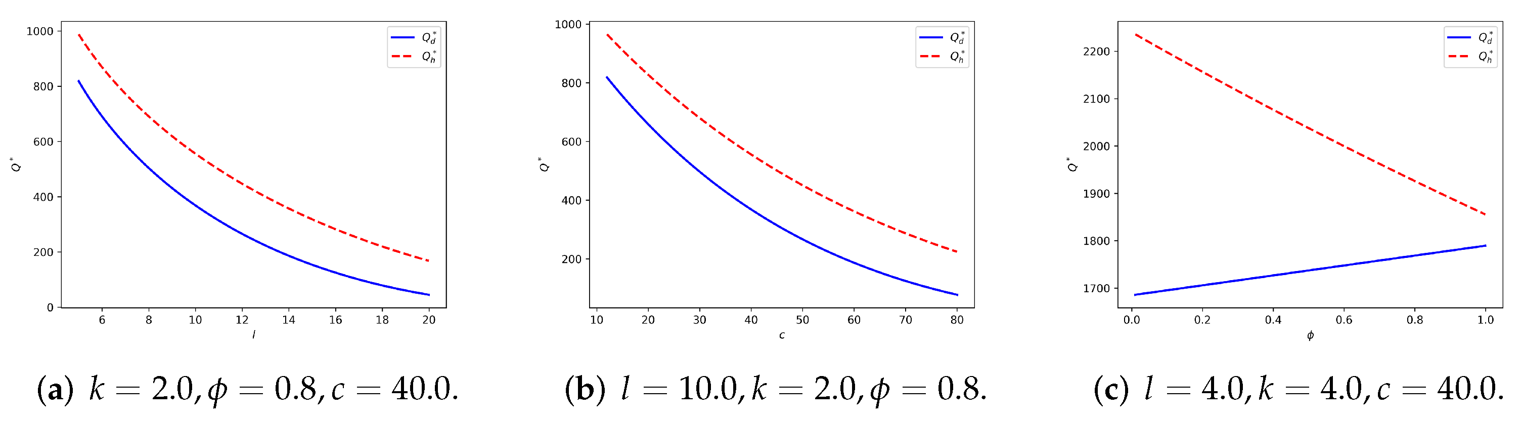
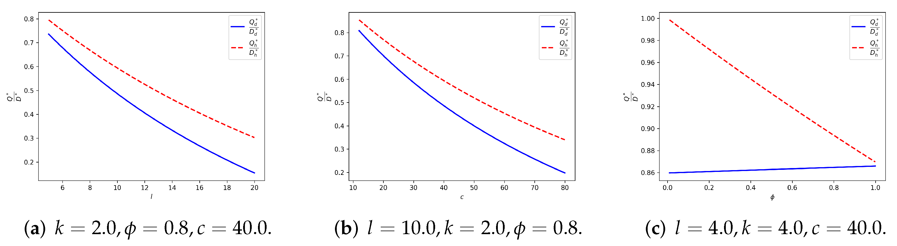
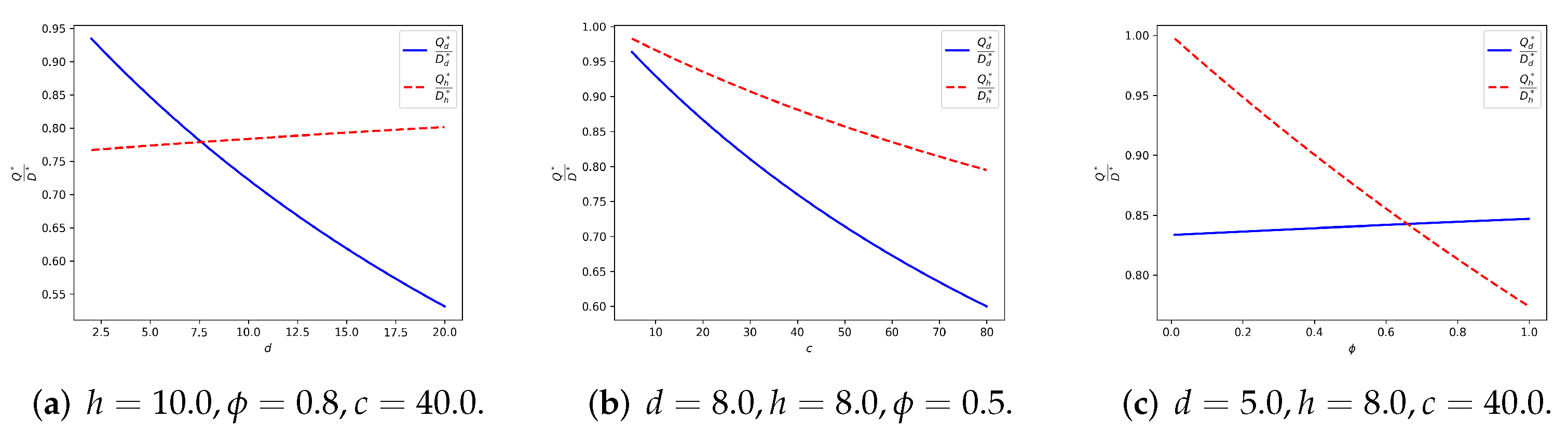
- is monotonically decreasing with c and increasing with ϕ.
- is monotonically decreasing with c and ϕ.
4.3.1. Symmetric Linear Demand
4.3.2. Seller-Reliant Linear Demand
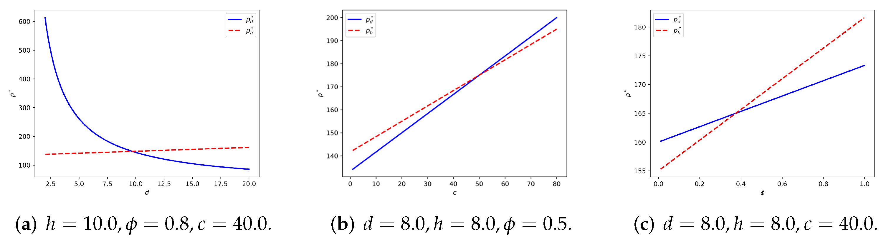
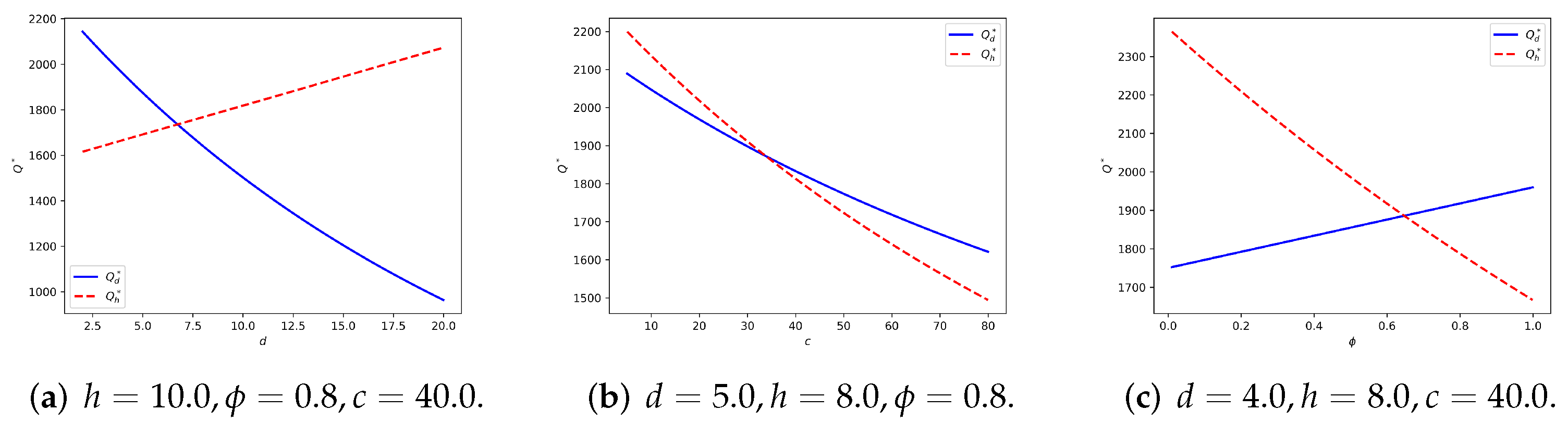
- is monotonically decreasing with d and increasing with h, is monotonically decreasing with h and increasing with d.
- is monotonically decreasing with d and increasing with h, is monotonically decreasing with h and increasing with d.
- If , that is, in the market, the drugstore has an influence at least twice that of the hospital. We obtain that is non-negative and is positive. Thus in this situation, the game will end up with .
- If , the drugstore has an influence of half or less than half that of the hospital. Under this circumstance. We obtain that is non-positive and is negative. Thus, at the equilibrium point, the hospital will have a lower selling price than the drugstore.
- If , we rewrite Equation (13) asDefine . Investigate the sign of Equation (13) is then equivalent to discuss the sign of on .Taking the derivative of on d, we have .So the minimum point of is .As , we know by the symmetry of that . In case 1 and 2, we have already shown that and , there must exist a unique such that . We could obtain by solving the equation , where and . The expression of is not important, what we are concerned about is that when , the game will have at the equilibrium point, and when , it will end up with .
5. Numerical Analysis
5.1. Symmetric Linear Demand
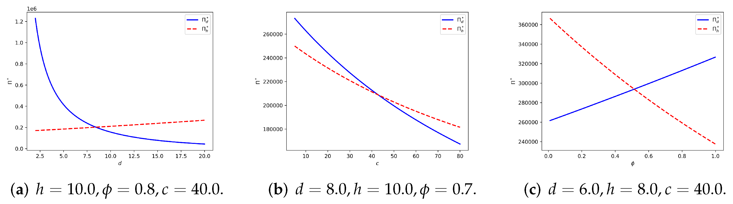
5.2. Seller-Reliant Linear Demand
6. Conclusions
6.1. Implications
6.2. Suggestions for Future Research
Author Contributions
Funding
Institutional Review Board Statement
Informed Consent Statement
Data Availability Statement
Acknowledgments
Conflicts of Interest
Appendix A. Proof of Lemmas and Theorems
Appendix A.1. Proof of Lemma 1
- Linear Form:For Assumption 3, .For Assumption 4, , thus and .
- Logarithmic Form:For Assumption 3, we have ,and .For Assumption 4, we have , then ,
Appendix A.2. Proof of Lemma 2
Appendix A.3. Proof of Lemma 3
Appendix A.4. Proof of Theorem 1
Appendix A.5. Proof of Lemma 4
Appendix A.6. Proof of Lemma 5
- NecessityAccording to definition, a function is called quasi-concave if holds for all .Assume f is neither monotonic nor first non-decreasing and then non-increasing. It means that is either first decreasing and increasing or first non-decreasing and then non-increasing but at last decreasing and increasing again. As is twice continuously differentiable, it is equivalent to say will cross 0 more than once.Let , be the two adjacent crossing points that satisfy . There exist a , for any , we have , where . Without loss of generality, we assume .
- IfBecause , we know that there exist a , such that for all , is strictly monotonic decreasing and all , is strictly monotonic increasing. This means that is convex on , which contracts the quasi-concavity of .
- IfSimilarly, we could say that there exist a , such that is convex on , which also contracts the quasi-concavity of .
Thus our assumption is wrong, which means is either monotonic or first non-decreasing and then non-increasing. - SufficiencyTake any , , without loss of generality, we assume .
- If is monotonic increasing, we have , then , thus is quasi-concave.
- If is monotonic decreasing, we have , then , thus is quasi-concave.
- If is first non-decreasing and then non-increasing. Let denote the turning point of , that is, for , is non-decreasing and , is non-increasing.
- (a)
- If , we have , then .
- (b)
- If , we have , then .
- (c)
- If , we will discuss the position of .
- If , we have , which means .
- If , we have , which means .
As discussed above, the sufficiency is proved.
Appendix A.7. Proof of Lemma 6
Appendix A.8. Proof of Theorem 2
Appendix A.9. Proof of Theorem 3
Appendix A.10. Proof of Theorem 4
Appendix A.11. Proof of Theorem 5
Appendix B. Equation Derivations
Appendix B.1. The Derivation of Equations (7) and (8)
Appendix B.2. The Derivation of Equation (A4)
References
- Imperatives, S. Report of the World Commission on Environment and Development: Our Common Future. 1987. Available online: http://www.ask-force.org/web/Sustainability/Brundtland-Our-Common-Future-1987-2008.pdf (accessed on 16 June 2022).
- Low, Y.S.; Halim, I.; Adhitya, A.; Chew, W.; Sharratt, P. Systematic framework for design of environmentally sustainable pharmaceutical supply chain network. J. Pharm. Innov. 2016, 11, 250–263. [Google Scholar] [CrossRef]
- Zahiri, B.; Zhuang, J.; Mohammadi, M. Toward an integrated sustainable-resilient supply chain: A pharmaceutical case study. Transp. Res. Part E Logist. Transp. Rev. 2017, 103, 109–142. [Google Scholar] [CrossRef]
- Kozlenkova, I.V.; Hult, G.T.M.; Lund, D.J.; Mena, J.A.; Kekec, P. The role of marketing channels in supply chain management. J. Retail. 2015, 91, 586–609. [Google Scholar] [CrossRef]
- Jraisat, L.; Upadhyay, A.; Ghalia, T.; Jresseit, M.; Kumar, V.; Sarpong, D. Triads in sustainable supply-chain perspective: Why is a collaboration mechanism needed? Int. J. Prod. Res. 2021, 1–17. [Google Scholar] [CrossRef]
- Sharma, M.; Kumar, A.; Luthra, S.; Joshi, S.; Upadhyay, A. The impact of environmental dynamism on low-carbon practices and digital supply chain networks to enhance sustainable performance: An empirical analysis. Bus. Strategy Environ. 2021, 31, 1776–1788. [Google Scholar] [CrossRef]
- Chen, X.; Jang, E. A Sustainable Supply Chain Network Model Considering Carbon Neutrality and Personalization. Sustainability 2022, 14, 4803. [Google Scholar] [CrossRef]
- Upadhyay, A. Antecedents of green supply chain practices in developing economies. Manag. Environ. Qual. Int. J. 2020. ahead of print. [Google Scholar] [CrossRef]
- NBS. Number of Health Care Institutions and Hospitals. 2000. Available online: https://data.stats.gov.cn/english/ (accessed on 16 June 2022).
- NBS. Number of Health Care Institutions and Hospitals. 2020. Available online: https://data.stats.gov.cn/english/ (accessed on 16 June 2022).
- Dong, H.; Bogg, L.; Rehnberg, C.; Diwan, V. Drug policy in China: Pharmaceutical distribution in rural areas. Soc. Sci. Med. 1999, 48, 777–786. [Google Scholar] [CrossRef]
- Yu, X.; Li, C.; Shi, Y.; Yu, M. Pharmaceutical supply chain in China: Current issues and implications for health system reform. Health Policy 2010, 97, 8–15. [Google Scholar] [CrossRef]
- Zixun, R. Out of Stock for Medicare Drugs? We Have Coordinated the Replenishment to the Hospital as Soon as Possible. 2021. Available online: https://baijiahao.baidu.com/s?id=1699934065210190979&wfr=spider&for=pc (accessed on 17 May 2021).
- Jiankang, X. Why the Methimazole Is Unavailable? Why Are Life-Saving Drugs Being Stocked Out? 2018. Available online: https://www.qcdy.com/m/view.php?aid=55805 (accessed on 5 June 2018).
- SohuNews. Drug Price Disparity! For Same Kind of Medicine, Drugstore Is Four or Five Times Expensive than Hospital. 2020. Available online: https://www.sohu.com/a/423564113_178984 (accessed on 10 October 2020).
- Chen, F.Y.; Yan, H.; Yao, L. A newsvendor pricing game. IEEE Trans. Syst. Man Cybern.-Part Syst. Hum. 2004, 34, 450–456. [Google Scholar] [CrossRef]
- Shah, N. Pharmaceutical supply chains: Key issues and strategies for optimisation. Comput. Chem. Eng. 2004, 28, 929–941. [Google Scholar] [CrossRef]
- Bollampally, K.; Dzever, S. The impact of RFID on pharmaceutical supply chains: India, China and Europe compared. Indian J. Sci. Technol. 2015, 8, 176–188. [Google Scholar] [CrossRef]
- Jæger, B.; Menebo, M.M.; Upadhyay, A. Identification of environmental supply chain bottlenecks: A case study of the Ethiopian healthcare supply chain. Manag. Environ. Qual. Int. J. 2021, 32, 1233–1254. [Google Scholar] [CrossRef]
- Ahmadi, A.; Mousazadeh, M.; Torabi, S.A.; Pishvaee, M.S. Or applications in pharmaceutical supply chain management. In Operations Research Applications in Health Care Management; Springer: Berlin/Heidelberg, Germany, 2018; pp. 461–491. [Google Scholar]
- Singh, R.K.; Kumar, R.; Kumar, P. Strategic issues in pharmaceutical supply chains: A review. Int. J. Pharm. Healthc. Mark. 2016, 10, 234–257. [Google Scholar] [CrossRef]
- Grunow, M.; Günther, H.O.; Yang, G. Plant co-ordination in pharmaceutics supply networks. OR Spectr. 2003, 25, 109–141. [Google Scholar] [CrossRef]
- Oh, H.C.; Karimi, I. Regulatory factors and capacity-expansion planning in global chemical supply chains. Ind. Eng. Chem. Res. 2004, 43, 3364–3380. [Google Scholar] [CrossRef]
- Sousa, R.T.; Shah, N.; Papageorgiou, L.G. Global supply chain network optimisation for pharmaceuticals. In Computer Aided Chemical Engineering; Elsevier: Amsterdam, The Netherlands, 2005; Volume 20, pp. 1189–1194. [Google Scholar]
- Sousa, R.T.; Liu, S.; Papageorgiou, L.G.; Shah, N. Global supply chain planning for pharmaceuticals. Chem. Eng. Res. Des. 2011, 89, 2396–2409. [Google Scholar] [CrossRef]
- Mousazadeh, M.; Torabi, S.A.; Zahiri, B. A robust possibilistic programming approach for pharmaceutical supply chain network design. Comput. Chem. Eng. 2015, 82, 115–128. [Google Scholar] [CrossRef]
- Zandkarimkhani, S.; Mina, H.; Biuki, M.; Govindan, K. A chance constrained fuzzy goal programming approach for perishable pharmaceutical supply chain network design. Ann. Oper. Res. 2020, 295, 425–452. [Google Scholar] [CrossRef]
- Papageorgiou, L.G.; Rotstein, G.E.; Shah, N. Strategic supply chain optimization for the pharmaceutical industries. Ind. Eng. Chem. Res. 2001, 40, 275–286. [Google Scholar] [CrossRef]
- Levis, A.A.; Papageorgiou, L.G. A hierarchical solution approach for multi-site capacity planning under uncertainty in the pharmaceutical industry. Comput. Chem. Eng. 2004, 28, 707–725. [Google Scholar] [CrossRef]
- Gatica, G.; Papageorgiou, L.; Shah, N. Capacity planning under uncertainty for the pharmaceutical industry. Chem. Eng. Res. Des. 2003, 81, 665–678. [Google Scholar] [CrossRef] [Green Version]
- Sundaramoorthy, A.; Evans, J.M.; Barton, P.I. Capacity planning under clinical trials uncertainty in continuous pharmaceutical manufacturing, 1: Mathematical framework. Ind. Eng. Chem. Res. 2012, 51, 13692–13702. [Google Scholar] [CrossRef]
- Sundaramoorthy, A.; Li, X.; Evans, J.M.; Barton, P.I. Capacity planning under clinical trials uncertainty in continuous pharmaceutical manufacturing, 2: Solution method. Ind. Eng. Chem. Res. 2012, 51, 13703–13711. [Google Scholar] [CrossRef]
- Naresh, S. Planning and Scheduling in Pharmaceutical Supply Chains. 2012. Available online: https://core.ac.uk/download/pdf/48659339.pdf (accessed on 16 June 2022).
- Mauderli, A.; Rippin, D. Production planning and scheduling for multi-purpose batch chemical plants. Comput. Chem. Eng. 1979, 3, 199–206. [Google Scholar] [CrossRef]
- Pinto, J.M.; Grossmann, I.E. A continuous time mixed integer linear programming model for short term scheduling of multistage batch plants. Ind. Eng. Chem. Res. 1995, 34, 3037–3051. [Google Scholar] [CrossRef]
- Grossmann, I.E.; Quesada, I.; Raman, R.; Voudouris, V.T. Mixed-integer optimization techniques for the design and scheduling of batch processes. In Batch Processing Systems Engineering; Springer: Berlin/Heidelberg, Germany, 1996; pp. 451–494. [Google Scholar]
- Blomer, F.; Gunther, H.O. LP-based heuristics for scheduling chemical batch processes. Int. J. Prod. Res. 2000, 38, 1029–1051. [Google Scholar] [CrossRef]
- Rogers, M.J.; Gupta, A.; Maranas, C.D. Real options based analysis of optimal pharmaceutical research and development portfolios. Ind. Eng. Chem. Res. 2002, 41, 6607–6620. [Google Scholar] [CrossRef]
- Blau, G.E.; Pekny, J.F.; Varma, V.A.; Bunch, P.R. Managing a portfolio of interdependent new product candidates in the pharmaceutical industry. J. Prod. Innov. Manag. 2004, 21, 227–245. [Google Scholar] [CrossRef] [Green Version]
- Varma, V.A.; Pekny, J.F.; Blau, G.E.; Reklaitis, G.V. A framework for addressing stochastic and combinatorial aspects of scheduling and resource allocation in pharmaceutical R&D pipelines. Comput. Chem. Eng. 2008, 32, 1000–1015. [Google Scholar]
- Colvin, M.; Maravelias, C.T. A stochastic programming approach for clinical trial planning in new drug development. Comput. Chem. Eng. 2008, 32, 2626–2642. [Google Scholar] [CrossRef]
- Colvin, M.; Maravelias, C.T. Modeling methods and a branch and cut algorithm for pharmaceutical clinical trial planning using stochastic programming. Eur. J. Oper. Res. 2010, 203, 205–215. [Google Scholar] [CrossRef]
- Antonijevic, Z. Optimization of Pharmaceutical R&D Programs and Portfolios: Design and Investment Strategy; Springer: Berlin/Heidelberg, Germany, 2014. [Google Scholar]
- Karaesmen, I.Z.; Scheller-Wolf, A.; Deniz, B. Managing perishable and aging inventories: Review and future research directions. In Planning Production and Inventories in the Extended Enterprise; Springer: Berlin/Heidelberg, Germany, 2011; pp. 393–436. [Google Scholar]
- Vila-Parrish, A.R.; Ivy, J.S.; King, R.E.; Abel, S.R. Patient-based pharmaceutical inventory management: A two-stage inventory and production model for perishable products with Markovian demand. Health Syst. 2012, 1, 69–83. [Google Scholar] [CrossRef]
- Uthayakumar, R.; Priyan, S. Pharmaceutical supply chain and inventory management strategies: Optimization for a pharmaceutical company and a hospital. Oper. Res. Health Care 2013, 2, 52–64. [Google Scholar] [CrossRef]
- Kelle, P.; Woosley, J.; Schneider, H. Pharmaceutical supply chain specifics and inventory solutions for a hospital case. Oper. Res. Health Care 2012, 1, 54–63. [Google Scholar] [CrossRef]
- Nicholas, C.P.; Dada, M. Pricing and the newsvendor problem: A review with extensions. Oper. Res. 1999, 47, 183–194. [Google Scholar]
- Qin, Y.; Wang, R.; Vakharia, A.J.; Chen, Y.; Seref, M.M. The newsvendor problem: Review and directions for future research. Eur. J. Oper. Res. 2011, 213, 361–374. [Google Scholar] [CrossRef] [Green Version]
- Whitin, T.M. Inventory control and price theory. Manag. Sci. 1955, 2, 61–68. [Google Scholar] [CrossRef]
- Mills, E.S. Uncertainty and price theory. Q. J. Econ. 1959, 73, 116–130. [Google Scholar] [CrossRef]
- Lau, A.H.L.; Lau, H.S. The newsboy problem with price-dependent demand distribution. IIE Trans. 1988, 20, 168–175. [Google Scholar] [CrossRef]
- Kabak, I.W.; Schiff, A. Inventory models and management objectives. Sloan Manag. Rev. 1978, 19, 53–59. [Google Scholar]
- Hadley, G.; Whitin, T.M. Analysis of Inventory Systems; Prentice Hall: Hoboken, NJ, USA, 1963. [Google Scholar]
- Nahmias, S.; Schmidt, C.P. An efficient heuristic for the multi-item newsboy problem with a single constraint. Nav. Res. Logist. Q. 1984, 31, 463–474. [Google Scholar] [CrossRef]
- Bernstein, F.; Federgruen, A. Decentralized supply chains with competing retailers under demand uncertainty. Manag. Sci. 2005, 51, 18–29. [Google Scholar] [CrossRef] [Green Version]
- Levi, R.; Perakis, G.; Uichanco, J. The data-driven newsvendor problem: New bounds and insights. Oper. Res. 2015, 63, 1294–1306. [Google Scholar] [CrossRef]
- Oroojlooyjadid, A.; Snyder, L.V.; Takáč, M. Applying deep learning to the newsvendor problem. IISE Trans. 2020, 52, 444–463. [Google Scholar] [CrossRef] [Green Version]
- Wang, Y. Joint pricing-production decisions in supply chains of complementary products with uncertain demand. Oper. Res. 2006, 54, 1110–1127. [Google Scholar] [CrossRef]
- Karlin, S.; Carr, C.R. Prices and optimal inventory policy. In Studies in Applied Probability and Management Science; Springer: Berlin/Heidelberg, Germany, 1962; pp. 159–172. [Google Scholar]
- Cachon, G.P.; Netessine, S. Game theory in supply chain analysis. In Supply Chain Analysis in the eBusiness Era; Simchi-Levi, D., Wu, S.D., Shen, Z.M., Eds.; Kluwer Academic: Norwell, MA, USA, 2003. [Google Scholar]
- Guillemin, V.; Pollack, A. Differential Topology; American Mathematical Society: Providence, RI, USA, 2010; Volume 370. [Google Scholar]
- Wuhan, M.H.S.A. Notice on Adjusting Some of the Online Drugs’ Information. 2022. Available online: http://ybj.wuhan.gov.cn/zwgk_52/ybdt/tzgg/202205/t20220527_1978163.shtml (accessed on 27 May 2022).
- Liuzhou, M.H.S.A. Notice: Some Special Medical Insurance Drugs Could Be Paid by Patient Co-Ordination Programme. 2022. Available online: http://www.liuzhou.gov.cn/lzybj/zwgk/fdzdgknr/zcwj/yldy/202206/t20220602_3070722.shtml (accessed on 2 June 2022).
- NDRC. China Organizes Pilot Programs of Drug Centralized Bidding and Purchasing Policy. 2019. Available online: http://www.gov.cn/zhengce/content/2019-01/17/content_5358604.htm (accessed on 17 January 2019).
- Parlar, M.; Goyal, S.K. Optimal ordering decisions for two substitutable products with stochastic demands. Opsearch 1984, 21, 1–15. [Google Scholar]


| Symbol | Description |
|---|---|
| c | Ex-factory price for the supplier |
| Discount factor for the hospital, where the hospital gets a marginal cost of , | |
| Selling price for the drugstore | |
| Selling price for the hospital | |
| Order quantity for the drugstore | |
| Order quantity for the hospital | |
| Optimal selling price for the drugstore | |
| Optimal selling price for the hospital | |
| Optimal order quantity for the drugstore | |
| Optimal order quantity for the hospital | |
| Reliability factor of the drugstore | |
| Reliability factor of the hospital | |
| Deterministic part of the drugstore’s demand, also represented as | |
| Deterministic part of the hospital’s demand, also represented as | |
| Price elasticity of the drugstore’s demand | |
| Price elasticity of the hospital’s demand | |
| Random part of the drugstore’s demand | |
| Density function of | |
| Cumulative distribution function of | |
| Random part of the hospital’s demand | |
| Density function of | |
| Cumulative distribution function of | |
| Best response function of the drugstore | |
| Best response function of the hospital | |
| Drugstore’s demand, where | |
| Hospital’s demand, where | |
| Expected payoff of the drugstore, also represented as | |
| Expected payoff of the hospital, also represented as | |
| Expected payoff of the supplier, also represented as |
Publisher’s Note: MDPI stays neutral with regard to jurisdictional claims in published maps and institutional affiliations. |
© 2022 by the authors. Licensee MDPI, Basel, Switzerland. This article is an open access article distributed under the terms and conditions of the Creative Commons Attribution (CC BY) license (https://creativecommons.org/licenses/by/4.0/).
Share and Cite
Wu, S.; Luo, M.; Zhang, J.; Zhang, D.; Zhang, L. Pharmaceutical Supply Chain in China: Pricing and Production Decisions with Price-Sensitive and Uncertain Demand. Sustainability 2022, 14, 7551. https://doi.org/10.3390/su14137551
Wu S, Luo M, Zhang J, Zhang D, Zhang L. Pharmaceutical Supply Chain in China: Pricing and Production Decisions with Price-Sensitive and Uncertain Demand. Sustainability. 2022; 14(13):7551. https://doi.org/10.3390/su14137551
Chicago/Turabian StyleWu, Suhan, Min Luo, Jingxia Zhang, Daoheng Zhang, and Lianmin Zhang. 2022. "Pharmaceutical Supply Chain in China: Pricing and Production Decisions with Price-Sensitive and Uncertain Demand" Sustainability 14, no. 13: 7551. https://doi.org/10.3390/su14137551
APA StyleWu, S., Luo, M., Zhang, J., Zhang, D., & Zhang, L. (2022). Pharmaceutical Supply Chain in China: Pricing and Production Decisions with Price-Sensitive and Uncertain Demand. Sustainability, 14(13), 7551. https://doi.org/10.3390/su14137551