Article

Close Interval Approximation of Pentagonal Fuzzy Numbers for Interval Data-Based Transportation Problems

1
Department of Mathematics, Faculty of Science, University of Peradeniya, Peradeniya 20400, Sri Lanka
2
Faculty of Computer Science and Information Technology, Universiti Tun Hussein Onn Malaysia, Batu Pahat 86400, Johor, Malaysia
3
Department of Industrial Engineering, Prince Sattam Bin Abdulaziz University, Al Kharj 16273, Saudi Arabia
4
Department of Mathematics, Jahangirnagar University, Savar, Dhaka 1342, Bangladesh
5
Department of Medical Instruments Engineering Techniques, Dijlah University College, Baghdad 10021, Iraq
6
Department of Medical Instruments Engineering Techniques, Al-Farahidi University, Baghdad 10021, Iraq
7
Department of Mechanical Engineering, Faculty of Engineering (Shoubra), Benha University, Cairo 11629, Egypt
*
Author to whom correspondence should be addressed.
Sustainability 2022, 14(12), 7423; https://doi.org/10.3390/su14127423
Submission received: 30 April 2022 / Revised: 10 June 2022 / Accepted: 14 June 2022 / Published: 17 June 2022

Abstract

:
Due to globalization in this modern age of technology and other uncontrollable influences, transportation parameters can differ within a certain range of a given period. In this situation, a managerial position’s objective is to make appropriate decisions for the decision-makers. However, in general, the determination of an exact solution to the interval data-based transportation problem (IDTP) becomes an NP-hard problem as the number of choices within their respective ranges increases enormously when the number of suppliers and buyers increases. So, in practice, it is difficult for an exact method to find the exact solution to the IDTP in a reasonable time, specifically the large-sized problems with large interval sizes. This paper introduces solutions to the IDTP where supply, demand, and cost are all in interval numbers. One of the best interval approximations, namely the closed interval approximation of pentagonal fuzzy number, is proposed for solving the IDTP. First, in the proposed closed interval approximation method (Method-1), the pentagonal fuzzification method converts the IDTP to a fuzzy transportation problem (FTP). Subsequently, two new ranking methods based on centroid and in-center triangle concepts are presented to transfer the pentagonal fuzzy number into the corresponding crisp (non-fuzzy) value. Thereafter, the optimal solution was obtained using Vogel’s approximation method coupled with the modified distribution method. The proposed Method-1 is reported against a recent method and shows superior performance over the aforementioned and a proposed Method-2 via benchmark instances and new instances.

1. Introduction

The transportation problem is a special class of linear programming problems that a transportation algorithm can solve. Optimization of the linear objective function is dealt with by linear programming, keeping in mind the linear constraints [1,2]. This method is also defined as the optimization of a function of variables. Many methods determine the initial basic feasible solution for balanced transport as in [3,4,5,6,7]. The transportation algorithm can be applicable only after identifying a feasible or basic solution station problem to obtain the minimum cost of transportation [8,9]. As everyone is interested in using the best possible resources to optimize profit and cost, different transportation models exist in different forms. Various types of transportation problems are applied in the business world, and the transportation problem aims to find a way of carrying out this transfer of goods at the minimum total cost [10,11]. While discussing the conventional transportation problem, it is assumed that an informed decision-maker understands the value of transportation cost, supply, and demand. However, uncertainty is a common phenomenon in real-life situations. In real-life problems, some parameters of transportation problems are not always deterministic [12]. So certain data may be exact; some other data can be in fuzzy form or interval form. This interval form transportation problem is called the interval-based transportation problem. An interval-valued fuzzy transportation problem (FTP) is defined as one in which supply, demand, and cost are all in interval numbers. This type of problem (IDTP) is quite difficult to solve directly using the available methods. The interval must be converted to a crisp number to solve this type of transportation problem [9]. Note that IDTP differs from the traveling salesman problem (TSP). It is a mathematical problem in which one finds the shortest possible route that visits each city exactly once and returns to the origin city. However, transportation problems with flexible demand, supply, and cost are termed interval data-based transportation problems (IDTP) [13]. IDTP is a mathematical problem that determines the optimal cost of shipment.
In a historical view of this topic, during their first paper on fuzzy set theory, Zadeh [14] and Goguen [15], the authors aimed to generalize the classical notion of a set and a proposition to accommodate fuzziness in a sense. It was the first and most meaningful momentum towards the mathematical formalization of fuzziness. In the real world, fuzzy numbers have become very useful. So many new methods and theories have been proposed to solve the FTP. One of the challenges in using mathematical programming is that the parameters in the problem formulation are not constants but rather fluctuating and uncertain. Despite extensive decision-making experience, the policymaker cannot always articulate the goals precisely. Decision-making in a fuzzy environment, developed by Bellman and Zadeh [16], improved and was a great help in the management of decision problems. The fuzzy set theory and its applications were proposed by Zimmermann [17]. The inclusion of an uncertain environment raised a new model of transportation problems abbreviated by FTP.
Pandian and Natarajan [18] proposed a new algorithm, namely the fuzzy zero-point method. By assuming that the parameters of the transportation problem are expressed by generalized trapezoidal fuzzy numbers, Kaur and Kumar [19] provided a new method to solve FTP based on a ranking function. In the latest report, Kaur and Kumar [20] investigated a specific sort of FTP. In that study, transportation costs were represented by generalized trapezoidal fuzzy numbers. They used a ranking function to adapt some conventional approaches to identify the first basic feasible and fuzzy optimal solutions. The proposed technique is based on a traditional approach, making it simple to comprehend and apply to real-world transportation issues for decision-makers. Rajarajeswari and Sudha [21] proposed a new method for the in-center of centroids and used Euclidean distance to rank generalized hexagonal fuzzy numbers. Ebrahimnejad [22] proposed a new method for solving FTPs. Generalized trapezoidal fuzzy values represent transportation costs in this method [23]. Pathinathan and Ponnivalavan [24] defined reverse-order triangular fuzzy numbers and reverse-order pentagonal fuzzy numbers (PFNs). Helan and Uma [25] introduced a new operation for the addition, subtraction, and multiplication of pentagon fuzzy numbers. They proposed a new method for ranking pentagon fuzzy numbers using the in-center of the centroids.
Panda and Pal [26] proposed the logical definition of developing a PFN, along with its arithmetic operation. Mathur et al. [27] developed a method based on trapezoidal fuzzy numbers to optimize transportation problems in a fuzzy environment. Maliniand and Ananthanarayanan [28] presented a new ranking method. Hunwisai and Kuman [29] introduced the method for solving FTPs using Robust’s ranking technique. They have used the allocation table method to find an initial basic feasible solution (IBFS) for the FTP.
Purushothkumar and Ananthanarayanan [30] introduced a new method for solving a wide range of such problems. Mondal and Mandal [31] presented an adaption of a PFN. Samuel and Raja [32] proposed a new algorithmic method to solve the unbalanced FTP. Rosline and Dison [33] developed the geometrical representation of symmetric PFNs and quadratic PFNs. Maheswari and Ganesan [34] proposed a method to solve the FTP.
Han et al. [35] propose fuzzy mathematics forms, which is a branch related to fuzzy set theory and fuzzy logic. Researchers in the field offer diverse methods that support creating many distinct models of traditional linear programming issues from which can obtain fuzzy solutions to the former problem. Many researchers have examined transportation problems with fuzzy cost coefficients and translated them to a bi-criteria problem with a crisp objective function [22]. Ashour [36] introduced two cost-minimization fuzzy transportation issues with hexagonal fuzzy numbers considering supplies and demand. Based on the ranking of generalized trapezoidal fuzzy numbers. Stankovićet al. [37] suggested a method for road traffic fuzzy risk analysis. The suggested method considers the centroid points and standard deviations of generalized trapezoidal fuzzy numbers to sort out universal trapezoidal fuzzy numbers. Helen and Uma [38] applied an evolutionary method to solve problems with fuzzy coefficients in transportation. Bisht and Srivastava [13] proposed a new ranking technique based on the in-center concept. Rabinson and Chandrasekaran [39] proposed a method for solving the TP problem with PFNs based on the ranking function. Uddin et al. (2021) introduced multi-objective transportation problems (MOTPs) in unpredictable environments and suggested a fuzzy membership function strategy based on goal programming. Chen et al. [2] presented a new framework to precisely predict short-term traffic flow from historical data. Zheng et al. [40] utilized a hyper-heuristic solution method for emergency railway transportation during the 2013 Dingxi earthquake in China.
In this paper, two distinct new methods (methods 1 and 2) are proposed to solve interval-based transportation problems. To illustrate the proposed method and to investigate the potential significance, ten numerical examples of interval-based transportation problems are solved, and obtained results are compared with the results of an existing method. The leading attainments of the designed study are shortened as follows:
  • The Interval data-based transportation problem (IDTP) is investigated;
  • Two new methods are proposed based on the following two key ideas:
    • Proposing a unique pentagonal fuzzification method (PFM) for fuzzifying interval data;
    • Proposing two new ranking methods (Method-1 and Method-2) to convert fuzzy numbers of FTPs into crisp values.
The rest of the paper is organized in the following manner: Section 2 describes the preliminaries and the mathematical formulation of the Interval data-based and FTPs. Development of the methods for solving the IDTP is provided in Section 3. Verification of the proposed methods via numerical examples is presented in Section 4. Finally, in Section 5, a conclusion has been drawn.

2. Materials and Methods

2.1. Preliminaries

Figure 1 represents the interval data-based transportation problem (IDTP), where a homogeneous product’s demands and supply capacities and unit transportation cost may not be known precisely but vary within an interval. Thus, the determination of the exact solution to the problem is challenging. The following nomenclature describes the preliminaries of this work.
Definition 1.
In a fuzzy set  A ˜ , each element is mapped to [0,1] by a membership function, μ A ˜ ( x ) , as follows:
  • μ A ˜ ( x ) :   [ 0 , 1 ] , have the following properties:
  • μ A ˜ ( x )  is an upper semi-continuous membership function;
  • A ˜  is a convex fuzzy set, i.e.,  μ A ˜ ( δ is   ( 1 δ )   y ) min { μ A ˜ ( x ) ,   μ A ˜ ( y ) }  for all  x ,   y ; 0 δ 1 ;
  • A ˜  is normal, i.e.,  x 0  for which  μ A ˜ ( x 0 ) = 1 .
Supp   ( A ˜ ) = { x :   μ A ˜ ( x ) > 0   }  is the support of  A ˜ , and the closure  cl ( Supp ( A ˜ ) )  is a compact set.
Definition 2.
A fuzzy numberk* = (p,q,r,s,t) is said to be a linear symmetric PFN if its membership function is given by:
µ k * ( X ) = { w 2 ( x p q p ) ;     p x q w 2 + w 2 ( x q r q ) ; q x r 1 ;   x = r w 2 w 2 ( x r s r ) ; r x s w 2 ( t x t s ) ;     s x t 0 ,   otherwise
If w = 1, then the k* is called a normal PFN. Otherwise, it is said to be a non-normal fuzzy number.
In general, PFN is a 5-tuple subset of a five-parameter real number  . The middle point of a PFN k* is  r , and the left- and right-side points of  r  are  ( p , q )  and  ( s , t ) , respectively.

2.2. Pentagonal Fuzzy Number (PFN)

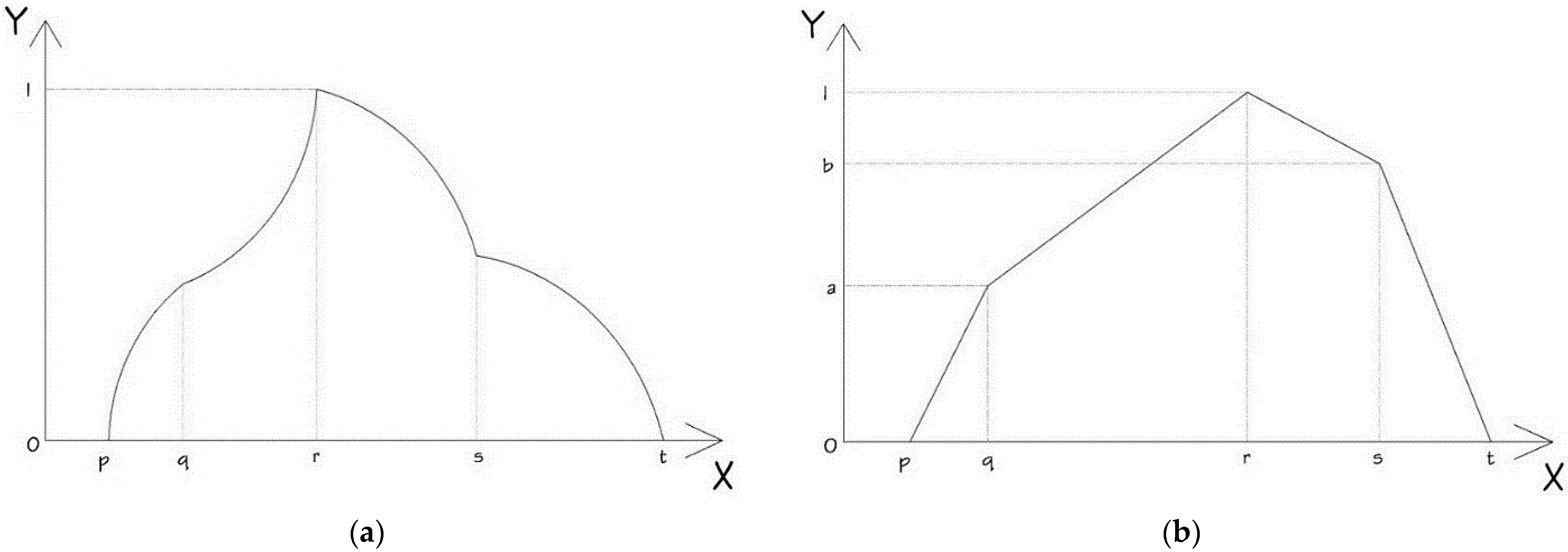
Based on Figure 2a,b, consider that the fuzzy number k* = {p, q, r, s, t} on R is said to be a PFN that should satisfy the following properties:
  • µk*(X) is a continuous function in the interval [0,1];
  • µk*(X) is a strictly increasing and continuous function on [p,q] and [q,r];
  • µk*(X) is a strictly decreasing and continuous function on [r,s] and [s,t].
For asymmetry, fuzzy numbers may be a > b or a < b. If a = b, the asymmetry fuzzy number becomes symmetry fuzzy numbers.
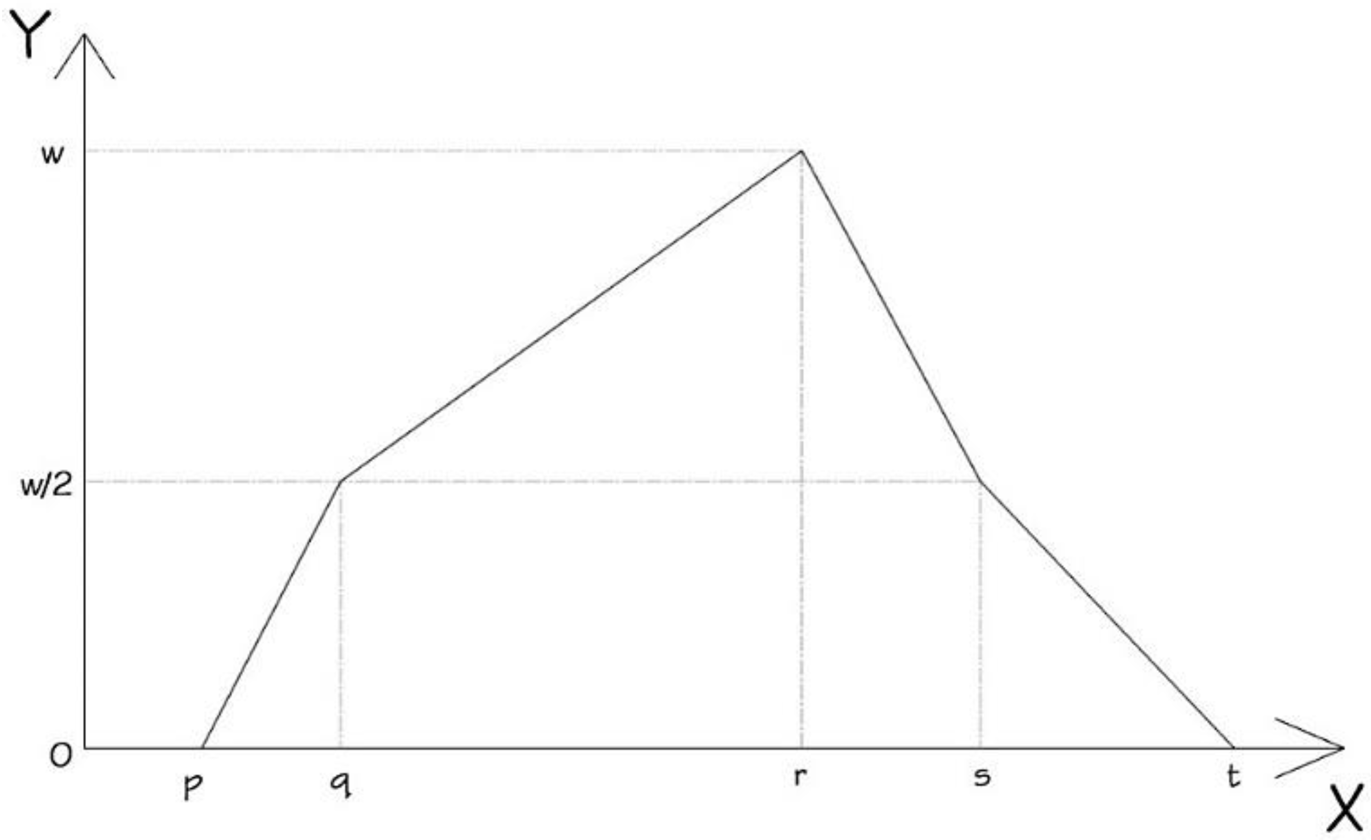
Let linear symmetry PFN k* = {p, q, r, s, t}, whose membership function is written as:
µ k * ( X ) = { w 2 ( x p qpn ) ;     par   sy w 2 + w 2 ( x   r   ) ; q   par   1 ;   x = r w 2 w 2 ( x ;   s ;   ) ; r   x = r   w 2 ( tr   tr   ) ;     s = r   sy 0 ,   otherwise
If w = 1, then k* is called a normal PFN, as shown in Figure 3. Otherwise, it is said to be a non-normal fuzzy number.

2.3. Properties of Pentagonal Fuzzy Numbers

Let P = {p1, p2, p3, p4, p5} and S = {s1, s2, s3, s4, s5} be two PFNs. Then, the fuzzy numbers addition, fuzzy numbers subtraction and fuzzy numbers multiplication are given by:
  • Addition: P + S = {p1 + s1, p2 + s2, p3 + s3, p4 + s4, p5 + s5};
  • Subtraction: P − S = {p1 − s1, p2 − s2, p3 − s3, p4 − s4, p5 − s5};
  • Multiplication: P × S   = { p 1 5 β , p 2 5 β ,   p 3 5 β ,   p 4 5 β , p 5 5 β }, where β = {p1 + p2 + p3 + p4 + p5};
  • Division: P ÷ Q = { 5 p 1 β , 5 p 2 β ,   5 p 3 β ,   5 p 4 β , 5 p 5 β } , where β = {p1 + p2 + p3 + p4 + p5} and β 0;
  • Scalar multiplication: αP = {αp1 + αp2 + αp + αp4 + αp5} where α ϵ R.
(For more details (refer to [31]), PFNs, their properties, and application in the fuzzy equation.)

2.4. The Formulation of the IDTP

The interval parameters (supply, demand, and unit transportation cost) are converted to fuzzy numbers using the proposed pentagonal fuzzification method (PFM) (as explained in Section 3). A fuzzy number is a quantity whose value is uncertain, such as transportation costs, demand, and supply.
Min i = 1 m j = 1 n c i j x i j
Subject to j = 1 n x i j s ; i = 1 , 2 , m and i = 1 m x i j d j ; j = 1 , 2 , n
Then,
i = 1 m s i j = 1 m d j
where S i s i S i i ; D j d j D j j ; C i j c i j C i j ;   x i j 0 , i , j .

2.5. Fuzzy Transportation Problems (FTP)

Mathematically, the FTP can be formulated as follows:
Min   Z ˜ = i = 1 n j = 1 m c ˜ i j x i j
Subject to
j = 1 m x i j   a ˜ i ;   i = 1 , 2 , , n i = 1 n x i j   b ˜ j   ; j = 1 , 2 , , m ;
where c ˜ i j   , a ˜ i , and b ˜ j are PFNs. Without a loss of generality, it is assumed that a ˜ i > 0 ,   b ˜ j > 0 , c ˜ i j   0 for all ( i ,   j )   and j = 1 n b ˜ j = i = 1 n a ˜ i , x i j 0     i = 1 , 2 , , n   ;   j = 1 , 2 , , m .
Definition 3. 
The feasible point x 0 is called a pentagonal fuzzy optimal solution to the FTP problem if and only if there does not exist another  x such that:
Z ˜ ( x i j ,   c ˜ i j   ) Z ˜ ( x i j 0 ,   c ˜ i j   ) ,   and   Z ˜ ( x i j ,   c ˜ i j   ) Z ˜ ( x i j 0 ,   c ˜ i j   ) ,

3. The Proposed Pentagonal Fuzzification Methods (PFM) for Solving the IDTP

The IDTP is a transportation problem where the transportation cost, demand, and supply are available in interval form because the decision-maker does not possess exact information.
The interval data of our concerned IDTP is fuzzified to a fuzzy number to apply the fuzzy technique as follows:
Let us consider an interval data P = (p,t), Defined = (t − p)/4. Then, P = (p, p + d, p + 2d, p + 3d, t) be a PFN.
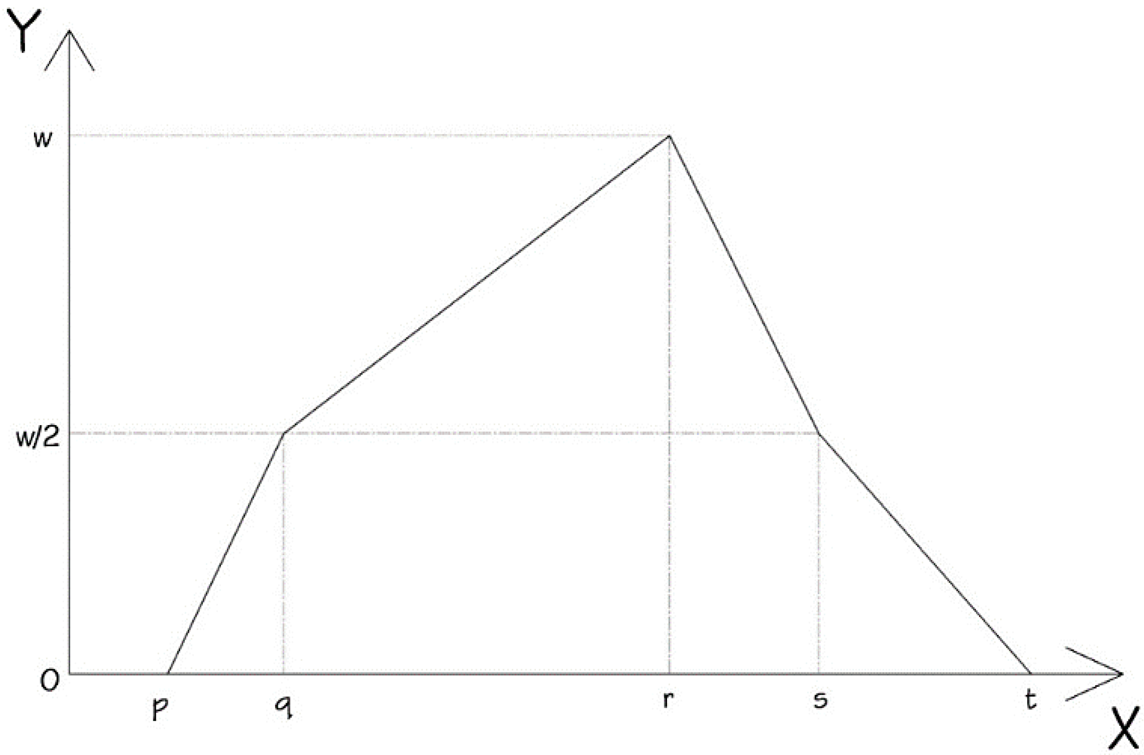
The arithmetic mean position of all the points in a surface diagram is called the centroid or geometric center. Informally, it is the point at which a cutout of the shape could be perfectly balanced on the tip of a pin. Consider normal PFN k * = (p, q, r, s, t) such that its centroid is ( x ^ ,   y ^ ) . Figure 4 shows a linear symmetry PFN when w = 1.
µ k * ( X ) = { 1 2 ( x p q p ) ;     p x q 1 2 + 1 2 ( x q r q ) ; q x r 1 ;   x = r 1 2 1 2 ( x r s r ) ; r x s 1 2 ( t x t s ) ;     s x t 0 ,   other   wise
Then, using the membership function and according to the centroid formula:
x ^ = x p q ( x p ) 2 ( q p ) dx   + x q r ( 1 2 + ( x q ) 2 ( r q ) ) dx + x r s ( 1 2 ( x r ) 2 ( s r ) ) dx + x s t ( t x ) 2 ( t s ) dx p q ( x p ) 2 ( q p ) dx   + q r ( 1 2 + ( x q ) 2 ( r q ) ) dx + r s ( 1 2 ( x r ) 2 ( s r ) ) dx + s t ( t x ) 2 ( t s ) dx ,
x ^ = 1 12 { p 2 2 q 2 + 3 r 2 s 2 + t 2 q ( p + r ) + s ( r + t ) } 1 4 { p 2 q + 2 r + t } , x ^ = 1 3 { p 2 2 q 2 + 3 r 2 s 2 + t 2 q ( p + r ) + s ( r + t ) } { p 2 q + 2 r + t }
where x ^ is the X-axis value of the centroid.
For a normal PFN k* = {p, q, r, s, t}, the ranking function R(P) is defined by
R(P) = x ^ .
Therefore, R(P) = 1 3 { p 2 2 q 2 + 3 r 2 s 2 + t 2 q ( p + r ) + s ( r + t ) } { p 2 q + 2 r + t } .
For any two PFNs, P = {p1, p2, p3, p4, p5} and S = {s1, s2, s3, s4, s5}, then:
  • P S ⇔ R(P) R(S);
  • P S ⇔ R(P) R(S);
  • P = S ⇔ R(P) = R(S).

3.1. Proposed Method-1

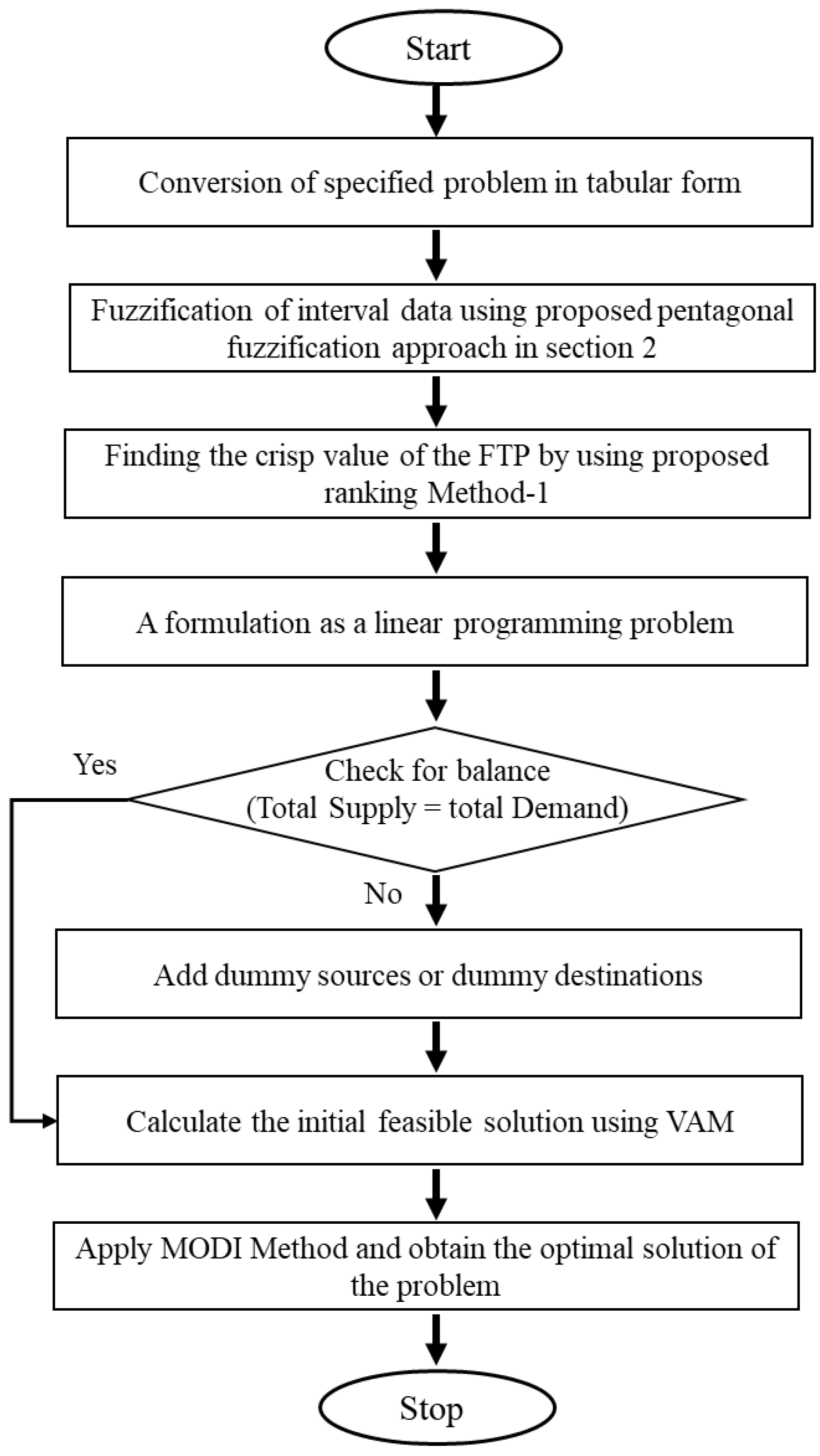
Here, at first, our IDTP is converted to the FTP using the PFM illustrated in Section 3. Then, a new ranking method based on the centroid concept is developed to convert the PFN into a crisp value. Finally, Vogel’s Approximation Method (VAM) coupled with the modified distribution method (MODI) is utilized to attain the optimal solution. Based on this notion, the following fuzzy technique is presented to solve an IDTP (interval data-based transportation problem). The following steps are followed to solve an IDTP:
  • Step 1: Transforming the specified problem in tabular form;
  • Step 2: Fuzzifying data using the proposed PFM in Section 3;
  • Step 3: Finding the crisp value of the FTP (model 2) using the proposed ranking Method-1;
  • Step 4: Formulating a linear programming problem and checking for the balance;
  • Step 5: Calculating the initial feasible solution using VAM;
  • Step 6: Finally, applying the MODI and obtaining the optimal solution to the problem.
For a better understanding of the above computational method, a flow chart is presented in Figure 5. A benchmark example 1 of [13] is provided below for exploring the efficiency of the described IDTP along with the appropriateness of Method-1 in Section 4.

3.2. Proposed Ranking Method-2

The in-center is one of the triangle’s points of concurrency formed by the intersection of the triangle’s three-angle bisectors. Consider the normal PFN P = (p, q, r, s, t), as in Figure 6.
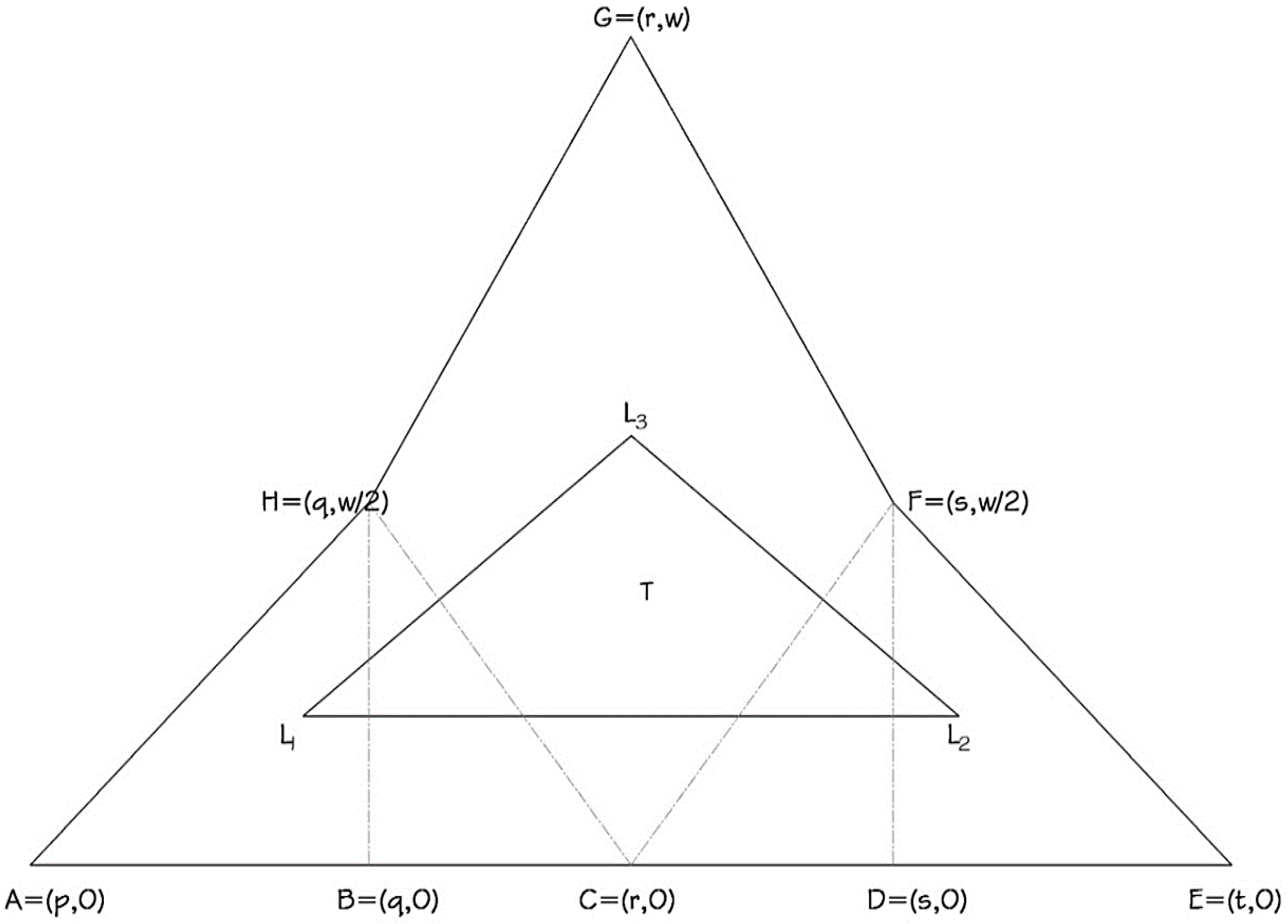
It can be easily observed from Figure 6 that we divide the pentagon, AEFGH, into three planes: ACH, CEF, and CFGH. Let the centroid of these three plane figures be L1, L2, and L3, respectively. Then,
  • L1 = p + q + r 3 , w 6 ;
  • L2 = r + s + t 3 , w 6 ;
  • L3 = q + 2 r + s 4 , w 2 .
Since L1L2L3 is a triangle, the in-center T of this triangle with vertices L1, L2, and L3 can be defined as Centre, T = (x, y), as shown in Figure 7, and formulated in the following.
x = cx 1 + bx 2 + ax 3 a + b + c
where x is the X-axis value of the in-center, and   a = s + t p q 3 , b = ( 4 p + q 2 r 3 s ) 2 + 16 w 2 12 , and c = ( 4 t + s 2 r 3 q ) 2 + 16 w 2 12 . The ranking function R(P) is given by R(P) = x. Therefore,
R ( P ) = cx 1 + bx 2 + ax 3 a + b + c
Here, w = 1; P = (p, q, r, s, t) is a normal PFN.

3.3. Proposed Method-2

Our IDTP is first converted to the FTP using the PFM provided in Section 3. Then, a new ranking method based on the in-center of a triangle concept is presented to transfer the PFN into the crisp value. Finally, VAM coupled with the MODI is applied to obtain the optimal solution. For a better understanding of the above computational Method-2, a flow chart is presented below in Figure 8.
Based on the notions provided in Figure 8, the following fuzzy technique is proposed to solve the IDTP:
  • Step 1: Transforming a specified problem into tabular form;
  • Step 2: Fuzzifying interval data using the proposed PFM in Section 3;
  • Step 3: Finding the crisp value of the FTP (model 2) using the proposed ranking Method-2;
  • Step 4: Formulating a linear programming problem and checking for the balance;
  • Step 5: Calculating the initial feasible solution using VAM;
  • Step 6: Finally, applying the MODI and obtaining the optimal solution to the problem.
A benchmark example 2 of [13] is provided for investigating the efficiency of the described IDTP along with the appropriateness of our proposed Method-2 in Section 4.

4. Results and Discussion

To investigate the efficiency of the described IDTP along with the appropriateness of Method-1 and Method-2, in this section, the results of two benchmark examples of [13] are provided.

4.1. Using the Proposed Method-1

The following two benchmark instances (examples 1 and 2 of [13]) are solved by Method-1 proposed in this paper.
In this example, the initial feasible basic solution equals 154.16. The optimal solution for the problem using MODI is obtained following the provided steps. The results are shown at the bottom of Table 1. The minimum transportation cost equals 152.25 for this solution. Subsequently, Table 2 shows example 2 adopted from [13].
In this example, the initial feasible basic solution equals 93.38. The optimal solution for the problem using MODI is obtained after following the provided steps. The results are as shown at the bottom of Table 2. The minimum transportation cost equals 93.38 for this solution.

4.2. Using the Proposed Method-2

Our proposed Method-2 for this paper solves the first benchmark instance adopted from [13], as shown in Table 3.
In this example, the initial feasible basic solution equals 206.00. The optimal solution for the problem using MODI is obtained after following the provided steps. The results are as shown at the bottom of Table 3. The minimum transportation cost equals 206.00 for this solution.

4.3. Comparative Study

The solutions of both the benchmark examples of [13] were compared with our new proposed methods, and the results are provided in Table 4. To further illustrate the benefits of our proposed methods (Method-1 and Method-2) over the existing methods, we consider eight additional numerical example problems whose characteristics are detailed in Appendix A.
It can easily be observed from Table 4 that the solution obtained by our proposed Method-1 is better compared to the existing one and another proposed Method-2. Thus, we can claim that our proposed method outperforms the other two methods.

4.4. Statistical Analysis

Statistical significance of the average performance between the proposed method and the existing methods was evaluated using paired t-tests as the sample differences did assume the normal distribution. The null and alternative hypotheses for the test are defined as follows:
H0: 
There is no performance difference between the proposed method and the existing method.
H1: 
The proposed method has a better performance than the existing method.
The mean differences, along with the 95% confidence interval between the performance of existing methods and the proposed method, are summarized in Table 5.
In the above table, the p-values for the comparisons are less than 0.05. This indicates a statistically significant difference in the mean performance between the existing and the proposed method. Additionally, the mean differences of the total costs found by comparisons are positive, which indicates that the proposed method leads to a lower value than the existing method. Similar conclusions could be made by looking at the 95% confidence intervals as they do not contain 0 within limits. For example, with 95% confidence, we can conclude that the true mean performance difference between the proposed Method-1 and the Bisht and Srivastava method falls within 17.81 and 59.44 limits.

5. Conclusions

In this paper, the IDTP has been investigated with minimal cost of transportation by developing a new model where the unit cost of transportation, supply, and demand parameters has been considered in the form of intervals. This paper puts forward a combination of two new ideas to solve the IDTP. Firstly, IDTP is converted to FTP using a proposed fuzzy pentagonal method (FPM), and secondly, a newly proposed two ranking techniques based on centroid and in-center of triangle concepts are applied for switching to crisp numbers. Following these, two distinct new fuzzy methods are proposed for solving the IDTP. The comparative study via benchmark instances and some randomly generated ones shows that ranking Method-1 performs much better than Bisht and Srivastava’s [13] method and ranking Method-2. The merit of the proposed ranking Method-1 is highlighted. The proposed fuzzy methods are found to be more effective in solving such IDTP, which has a large difference in the intervals of production and demand. This scheme suggests considerable industrial and engineering applications in decision-making. Although our new ranking Method-1 outperforms the existing method in obtaining the minimal cost of small-sized IDTPs, it does not satisfy any large-sized IDTP instances. Moreover, the single-objective fuzzy or non-FTP cannot deal with real-life decision-making problems due to the current competitive market state. Therefore, we suggest future research to develop a streamlined method for solving large-sized interval-based multi-objective transportation problems. Another future work might be carried out to develop a new method that hybridizes the two ranking methods to obtain better results.

Author Contributions

Conceptualization, Z.A.M.S.J., S.A.M. and A.P.B.; methodology, A.A., M.S.U. and T.A.; software, E.-A.A., S.A.M. and M.M.J.; validation, A.A., M.S.U. and T.A.; formal analysis, Z.A.M.S.J., S.A.M. and A.P.B.; investigation, Z.A.M.S.J. and A.P.B.; resources, E.-A.A., S.A.M. and M.M.J.; data curation, A.A., M.S.U. and T.A.; writing—original draft preparation, Z.A.M.S.J., S.A.M. and M.S.U.; writing—review and editing, S.A.M. and Z.A.M.S.J.; visualization, E.-A.A., A.P.B. and M.M.J.; supervision, S.A.M. and Z.A.M.S.J.; project administration, S.A.M., Z.A.M.S.J. and M.S.U.; funding acquisition, E.-A.A., A.A., M.S.U. and T.A. All authors have read and agreed to the published version of the manuscript.

Funding

The authors extend their appreciation to the Deputyship for Research and Innovation, Ministry of Education in Saudi Arabia, for funding this research work through the project number (IF-PSAU-2021/01/18925).

Data Availability Statement

The used dataset of this research is available online and has a proper citation within the paper contents.

Acknowledgments

The authors would like to thank the Center of Intelligent and Autonomous Systems (CIAS) at the Faculty of Computer Science and Information Technology (FSKTM), UniversitiTun Hussein Onn Malaysia (UTHM), for supporting this work.

Conflicts of Interest

The authors declare that they have no conflict of interest to be addressed related to this work.

Nomenclature

a ˜ i Fuzzy supply value at i supply node
b ˜ j Fuzzy demand per unit time at j demand node
c ˜ i j   Unit fuzzy transportation cost from i supply node to j demand node
x i , j Number of units transported from i supply node to j demand node
nTotal number of supply nodes (suppliers)
mTotal number of demand nodes (buyers)
A ˜ convex fuzzy set
μ A ˜ ( x ) An upper semi-continuous membership function
k*Linear symmetric pentagonal fuzzy number
µk*(x)Pentagonal fuzzy membership function
S ^ Interval supply quantity (in units) from i supplier
d ^ Interval demand (in units) per unit time to j buyer
S _ Lower bound of supplies from the I supplier
S ¯ Upper bound of supplies from the i supplier
D _ Lower bound of demands of the j buyer
D ¯ Upper bound of demands of the j buyer
c ^ Interval unit transportation cost from i supply node to jdemand node

Appendix A

Table A1. Tabular form—example 3.
R1R2R3Supply
A[1,31][1,9][4,11][1,15]
B[3,33][1,31][5,23][2,12]
C[2,12][3,11][1,17][1,33]
Demand[4,22][1,9][5,23]
Table A2. Tabular form—example 4.
R1R2R3Supply
A[4,26][4,19][1,37][5,17]
B[3,35][2,6][1,13][4,24]
C[2,18][4,26][2,14][2,18]
Demand[1,12][5,17][3,15]
Table A3. Tabular form—example 5.
R1R2R3Supply
A[7,22][1,33][1,31][1,9]
B[2,34][5,23][4,19][2,29]
C[4,11][8,23][2,34][1,18]
Demand[1,17][5,35][1,33]
Table A4. Tabular form—example 6.
R1R2R3Supply
A[1,11][2,17][2,29][8,23]
B[3,35][5,25][6,32][1,21]
C[1,29][2,27][3,33][2,22]
Demand[3,31][2,29][2,24]
Table A5. Tabular form—example 7.
R1R2R3Supply
A[1,27][7,28][4,32][1,33]
B[3,33][1,33][1,31][2,18]
C[7,31][1,15][1,19][2,14]
Demand[1,19][4,32][5,17]
Table A6. Tabular form—example 8.
R1R2R3Supply
A[2,8][3,15][1,13][2,13]
B[3,11][2,10][2,13][1,19]
C[2,13][1,9][4,8][3,10]
Demand[1,21][2,10][3,12]
Table A7. Tabular form—example 9.
R1R2R3Supply
A[3,31][1,29][5,13][6,24]
B[5,20][5,25][1,31][1,35]
C[6,23][4,27][2,28][7,25]
Demand[3,28][1,33][4,32]
Table A8. Tabular form—example 10.
R1R2R3R4Supply
A[4,26][1,31][5,18][4,20][1,33]
B[2,24][5,20][2,27][1,31][4,30]
C[7,31][4,28][2,26][4,25][4,32]
Demand[1,31][4,29][4,20][2,28]

References

  1. Charkhgard, H.; Savelsbergh, M.; Talebian, M. A linear programming based algorithm to solve a class of optimization problems with a multi-linear objective function and affine constraints. Comput. Oper. Res. 2018, 89, 17–30. [Google Scholar] [CrossRef]
  2. Chen, X.; Wu, S.; Shi, C.; Huang, Y.; Yang, Y.; Ke, R.; Zhao, J. Sensing data supported traffic flow prediction via denoising schemes and ANN: A Comparison. IEEE Sens. J. 2020, 20, 14317–14328. [Google Scholar] [CrossRef]
  3. Juman, Z.A.M.S.; Nawarathne, N.G.S.A. An efficient alternative approach to solve a transportation problem. Ceylon J. Sci. 2019, 48, 19–29. [Google Scholar] [CrossRef] [Green Version]
  4. Juman, Z.A.M.S.; Hoque, M.A. An efficient heuristic to obtain a better initial feasible solution to the transportation problem. Appl. Soft Comput. 2015, 34, 813–826. [Google Scholar] [CrossRef]
  5. Bezmaternykh, A.; Kulizhskaya, Z.; Fayzrakhmanova, E. A Balanced System of Indicators as a Condition for Improving the Effectiveness of Management Decisions in the Field of Transport. Transp. Res. Procedia 2022, 61, 176–179. [Google Scholar] [CrossRef]
  6. Juman, Z.A.M.S.; Hoque, M.A.; Buhari, M.I.A. Sensitivity analysis and an implementation of the well-known Vogel’s approximation method for solving unbalanced transportation problems. Malays. J. Sci. 2013, 32, 66–72. [Google Scholar] [CrossRef]
  7. Chhibber, D.; Srivastava, P.K.; Bisht, D.C. From fuzzy transportation problem to non-linear intuitionistic fuzzy multi-objective transportation problem: A literature review. Int. J. Model. Simul. 2021, 41, 335–350. [Google Scholar] [CrossRef]
  8. Juman, Z.A.M.S.; Mostafa, S.A.; Ghazali, R.; Karunamuni, K.S.M.; Kumari, H.M.N.S. A Generalized Assignment of Standard Minute Value Model to Minimize the Difference between the Planned and Actual Outputs of a Garment Production Line. In International Conference on Soft Computing and Data Mining; Springer: Cham, Switzerland, 2022; pp. 272–281. [Google Scholar]
  9. Ahmed, J.S.; Mohammed, H.J.; Chaloob, I.Z. Application of a fuzzy multi-objective defuzzification method to solve a transportation problem. Mater. Today Proc. 2021. [Google Scholar] [CrossRef]
  10. Srivastava, P.K.; Bisht, D.; Garg, H. Innovative Ranking and Conversion Approaches to Handle Impreciseness in Transportation. J. Mult. -Valued Log. Soft Comput. 2020, 35, 491–507. [Google Scholar]
  11. Mostafa, S.A.; Juman, Z.A.M.S.; Nawi, N.M.; Mahdin, H.; Mohammed, M.A. Improving Genetic Algorithm to Attain Better Routing Solutions for Real-World Water Line System. In International Conference on Soft Computing and Data Mining; Springer: Cham, Switzerland, 2022; pp. 292–301. [Google Scholar]
  12. Zhu, K.; Ji, K.; Shen, J. A fixed charge transportation problem with damageable items under uncertain environment. Phys. A: Stat. Mech. Its Appl. 2021, 581, 126234. [Google Scholar] [CrossRef]
  13. Bisht, C.S.; Srivastava, P.K. Trisectional fuzzy trapezoidal approach to optimize interval data based transportation problem. J. King Saud Univ.-Sci. 2020, 32, 195–199. [Google Scholar] [CrossRef]
  14. Zadeh, L.A. Fuzzy sets. Inf. Control 1965, 8, 338–353. [Google Scholar] [CrossRef] [Green Version]
  15. Goguen, J.A. The logic of nexact concepts. Synthese 1969, 19, 325–373. [Google Scholar] [CrossRef]
  16. Bellman, R.E.; Zadeh, L.A. Decision making in a fuzzy environment. Manag. Sci. 1970, 17, 141–164. [Google Scholar] [CrossRef]
  17. Zimmermann, H.J. Fuzzy programming and linear programming with several objective functions. Fuzzy Sets Syst. 1978, 1, 45–55. [Google Scholar] [CrossRef]
  18. Pandian, P.; Natarajan, G. A new algorithm for finding a fuzzy optimal solution for fuzzy transportation problem. Appl. Math. Sci. 2010, 4, 79–90. [Google Scholar]
  19. Kaur, A.; Kumar, A. A new method for solving fuzzy transportation problems using ranking function. Appl. Math. Model. 2011, 35, 5652–5661. [Google Scholar] [CrossRef]
  20. Kaur, A.; Kumar, A. A new approach for solving fuzzy transportation problems using generalized trapezoidal fuzzy numbers. Appl. Soft Comput. 2012, 12, 1201–1213. [Google Scholar] [CrossRef]
  21. Rajarajeswari, R.; Sudha, A.S. A new approach for ranking of fuzzy numbers using the incentre of centroids. Int. J. Fuzzy Math. Arch. 2014, 4, 52–60. [Google Scholar]
  22. Ebrahimnejad, A. A simplified new approach for solving fuzzy transportation problems with generalized trapezoidal fuzzy numbers. Appl. Soft Comput. 2014, 19, 171–176. [Google Scholar] [CrossRef]
  23. Ebrahimnejad, A. A method for solving linear programming with interval-valued trapezoidal fuzzy variables. RAIRO-Oper. Res. 2018, 52, 955–979. [Google Scholar] [CrossRef] [Green Version]
  24. Pathinathan, T.; Ponnivalavan, K. Reverse order triangular, trapezoidal and pentagonal fuzzy numbers. Ann. Pure Appl. Math. 2015, 9, 107–117. [Google Scholar]
  25. Helen, R.; Uma, G.A. A new operation and ranking on pentagonal fuzzy numbers. Int. J. Math. Sci. Appl. 2015, 5, 2230–9888. [Google Scholar]
  26. Panda, A.; Pal, P. A study on pentagonal fuzzy number and its corresponding matrices. Pac. Sci. Rev. B Humanit. Soc. Sci. 2016, 1, 131–139. [Google Scholar] [CrossRef] [Green Version]
  27. Mathur, N.; Srivastava, P.K.; Paul, A. Trapezoidal fuzzy model to optimize transportation problem. Int. J. Model. Simul. 2016, 7, 1650028. [Google Scholar] [CrossRef]
  28. Maliniand, P.; Ananthanarayanan, M. Solving fuzzy transportation problem using ranking of trapezoidal fuzzy numbers. Int. J. Math. Res. 2016, 8, 127–132. [Google Scholar]
  29. Hunwisai, D.; Kuman, P. A method for solving a fuzzy transportation problem via Robust ranking technique and ATM. Cogent Math. 2017, 4, 1283730. [Google Scholar] [CrossRef]
  30. Purushothkumar, M.K.; Ananathanarayan, M. Fuzzy transportation problem of trapezoidal fuzzy numbers with new ranking technique. IOSR J. Math. 2017, 13, 6–12. [Google Scholar]
  31. Mondal, S.P.; Mandal, M. Pentagonal fuzzy numbers, its properties and application in fuzzy equation. Future Comput. Inform. J. 2017, 2, 110–117. [Google Scholar] [CrossRef]
  32. Samuel, A.; Raja, P. Algorithmic approach to unbalanced fuzzy transportation problem. Int. J. Pure Appl. Math. 2017, 113, 553–561. [Google Scholar]
  33. Rosline, J.J.; Dison, E.M. Symmetric pentagonal fuzzy numbers. Int. J. Pure Appl. Math. 2018, 119, 245–253. [Google Scholar]
  34. Maheswari, P.U.; Ganesan, K. Solving fully fuzzy transportation problem using pentagonal fuzzy numbers. J. Phys. 2018, 1000, 012014. [Google Scholar] [CrossRef] [Green Version]
  35. Han, D.; Cluckie, I.D.; Karbassioun, D.; Lowry, J. A fuzzy logic approach to river flow modelling. In Stochastic Hydraulics 2000; CRC Press: Boca Raton, FL, USA, 2020; pp. 853–860. [Google Scholar]
  36. Ashour, M.A.H. Optimum Cost of Transporting Problems with Hexagonal Fuzzy Numbers. J. Southwest Jiaotong Univ. 2019, 54. [Google Scholar] [CrossRef]
  37. Stanković, M.; Stević, Ž.; Das, D.K.; Subotić, M.; Pamučar, D. A new fuzzy MARCOS method for road traffic risk analysis. Mathematics 2020, 8, 457. [Google Scholar] [CrossRef] [Green Version]
  38. Helen, R.; Uma, G. A novel method to obtain initial basic solution and optimal solution of pentagonal fuzzy transportation problem. Malaya J. Mat. (MJM) 2019, 7, 676–680. [Google Scholar]
  39. Rabinson, G.C.; Chandrasekaran, R. A method for solving a pentagonal fuzzy transportation problem via ranking technique and ATM. Int. J. Res. Eng. IT Soc. Sci. 2019, 9, 71–75. [Google Scholar]
  40. Zheng, Y.J.; Zhang, M.X.; Ling, H.F.; Chen, S.Y. Emergency railway transportation planning using a hyper-heuristic approach. IEEE Trans. Intell. Transp. Syst. 2015, 16, 321–329. [Google Scholar] [CrossRef]
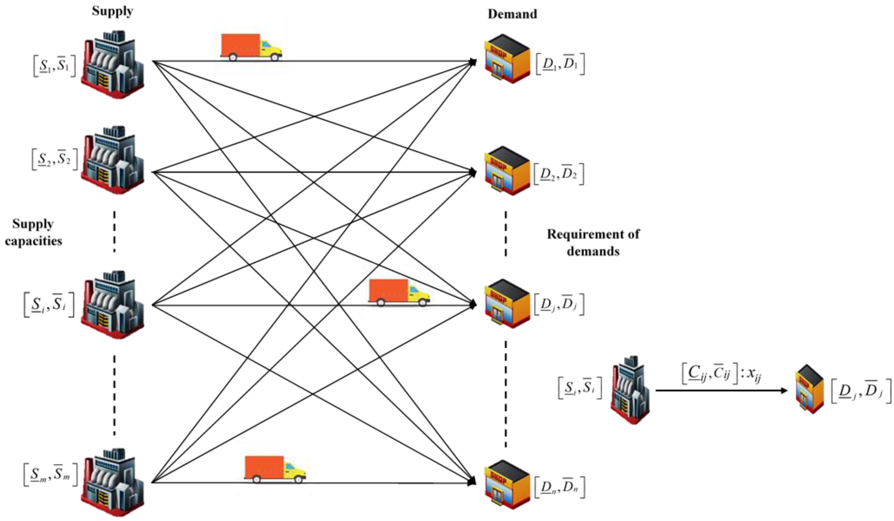
Figure 1. The interval data-based transportation problem.
Sustainability 14 07423 g001
Figure 2. (a) Nonlinear PFN and (b) linear asymmetry PFN.
Sustainability 14 07423 g002
Figure 3. Linear symmetry PFN.
Sustainability 14 07423 g003
Figure 4. Linear symmetry PFN when w equals 1.
Sustainability 14 07423 g004
Figure 5. Flowchart representation of the proposed Method-1.
Sustainability 14 07423 g005
Figure 6. Normal PFN.
Sustainability 14 07423 g006
Figure 7. Identifying the center to the proposed ranking Method-2.
Sustainability 14 07423 g007
Figure 8. Flowchart representation of the proposed Method-2.
Sustainability 14 07423 g008
Table 1. Tabular form of example 1.
R1R2R3Supply
Step 1: conversion of specified problem in tabular form
A[1,19][1,9][2,18][1,9]
B[8,26][3,12][7,28][4,10]
C[11,27][0,15][4,11][4,11]
Demand[3,12][4,10][2,8]
Step 2: Fuzzified interval data
A(1,5.5,10,14.5,19)(1,3,5,7,9)(2,6,10,14,18)(1,3,5,7,9)
B(8,10,12,14,16)(3,5.25,7.5,9.75,12)(7,12.25,17.5,22.75,28)(4,5.5,7,8.5,10)
C(11,15,19,23,27)(0,3.75,7.5,11.25,15)4,5.75,7.5,9.25,11)(4,5.75,7.5,9.25,11)
Demand(3,5.25,7.5,9.75,12)(4,5.5,7,8.5,10)(2,3.5,5,6.5,8)
Step 3: Defuzzified data
A9.254.679.334.67
B11.677.12516.626.75
C18.336.8757.217.21
Demand7.1256.924.75
Step 4: Balanced transportation problem
A9.254.679.334.67
B11.677.1316.626.75
C18.336.887.217.21
D0000.17
Demand7.136.924.75
Step 5: Initial basic feasible solution for the problem using VAM
A9.254.67    4.679.334.67
B11.67    6.757.1316.626.75
C18.33    0.216.88    2.257.21    4.757.21
D0    0.17000.17
Demand7.136.924.75
Table 2. Tabular form of example 2.
H1H2H3H4Supply
Step 1: Tabular form—example 2 with interval-based supplies and demands
L1[1,4][1,6][4,12][5,11][1,12]
L2[0,4][1,4][5,8][0,3][0,3]
L3[3,8][5,12][12,19][7,12][5,15.6]
Demand[5,10][1,10][1,6][1,4]
Step 2: Fuzzified interval data
L1(1,1.75,2.5,
3.25,4)
(1,2.25,3.5,
4.75,6)
(4,6,8,
10,12)
(5,6.5,8,
9.5,11)
(1,3.75,6.5,
9.25,12)
L2(0, 1, 2,
3, 4)
(1,1.75,2.5,
3.25,4)
(5,5.75,6.5,
7.25,8)
(0,0.75,1.5,
2.25,3)
(0,0.75,1.5,
2.25,3)
L3(3,4.25,5.5,
6.75,8)
(5,6.75,8.5,
10.25,12)
(12,13.75,15.5,
17.25,19)
(7,8.25,9.5,
10.75,12)
(5,7.65,10.3,
12.95,15.6)
Demand(5,6.25,7.5,
8.75,10)
(1,3.25,5.5,
7.75,10)
(1,2.25,3.5,
4.75,6)
(1,1.75,2.5,
3.25,4)
Step 3: Defuzzified data
A2.383.297.677.756.04
B1.832.386.381.381.38
C5.298.2115.219.299.86
Demand7.295.133.292.38
Step 4: Balanced transportation problem
A2.383.297.677.756.04
B1.832.386.381.381.38
C5.298.2115.219.299.86
D00000.81
Demand7.295.133.292.38
Step 5: Initial basic feasible solution for the problem using VAM
A2.383.29   3.567.67   2.487.756.04
B1.832.386.381.38   1.381.38
C5.29   7.298.21   1.5715.219.29   19.86
D000   0.8100.81
Demand7.295.133.292.38
Table 3. Tabular form of example 1.
R1R2R3Supply
Step 1: conversion of specified problem in tabular form
A[1,19][1,9][2,18][1,9]
B[8,26][3,12][7,28][4,10]
C[11,27][0,15][4,11][4,11]
Demand[3,12][4,10][2,8]
Step 5: Initial basic feasible solution for the problem using VAM
A205    5105
B17    77.517.57
C19    0.57.5    27.5    57.5
Demand7.575
Table 4. Comparative results.
ExampleBisht and Srivastava [13]Proposed Method-2Proposed Method-1
1154.93206152.25
293.39103.993.38
3272.5272.5237.89
4190.5190.5169.61
5337337294.71
6453.75453.75397.61
7483483422.2
8140.75140.75125.84
9612.75612.75545.51
10676.25676.25589.55
Table 5. Statistical significance of the average performance between the proposed methods and the existing methods.
ComparisonMean DifferenceStandard Error95% Confidence Interval for the Mean Differencep-Value
Bisht and Srivastava [13] Proposed Method-138.639.20(17.81, 59.44)0.002
Proposed Method-2
Proposed Method-1
44.797.80(27.14, 62.43)<0.001
Publisher’s Note: MDPI stays neutral with regard to jurisdictional claims in published maps and institutional affiliations.