Power Optimization Model for Energy Sustainability in 6G Wireless Networks

Abstract

Internet-of-Things (IoT) networks are witnessing a rapid proliferation of connected devices and mobile terminals each day. The wireless information flow between these massive battery-powered devices has a huge energy burden and will lead to an energy crisis in the near future; thus, there is an urgent search for sustainable energy networks. To offer a sustainable energy solution in order to meet the energy demands of these massive IoT networks, this paper presents a dynamic practical model that enables the efficient management of power resources. Two user-scheduling algorithms, namely, minimum distance scheduling (MDS) and maximum channel gain scheduling (MCS), are proposed; when these algorithms were used alongside a power optimization, they led to improved network efficiency. Further, the network’s performance was measured with parametric variations in the number of access points (APs); the deployment of APs and AP configuration is carried out for different precoding schemes. The impact of spatial correlation and the access to perfect channel state information (CSI) on the spectral efficiency of the system was also evaluated. In the end, the study compares the performance of different power-allocation methods and suggests that the power allocated to a particular user node by an AP can be controlled using the proposed algorithms. It is observed that, as compared to the MDS algorithm, the MCS algorithm results in better spectral efficiency for all the users with fractional power allocation. In addition, each AP assigns a maximum power of 141.7 mW to a user with strong channel conditions with the AP, and a minimum power of 3.1882 mW to the user with the worst channel conditions using centralized PMMSE precoding.

1. Introduction

Future wireless networks are envisioned for providing sustainable energy solutions to meet the ever-increasing energy demands of the massive number of connected devices and mobile terminals [1]. The battery-driven sensor nodes and connected equipments in an Internet-of-things (IoT) network consume a lot of power and put a huge burden on the energy consumption of the network. To strive for energy-saving capabilities in a connected network, sixth-generation (6G) sustainable networks are fast emerging to offer energy-efficient solutions [2,3,4]. At the same time, these future networks offer the advantages of low latency, massive connectivity, ultra reliability, and extreme traffic handling capabilities [5,6,7]. The techniques involved in 6G technology include small cells or cell densification [8], multi-antenna technology including multiple-input multiple-output (MIMO) and massive MIMO [9], millimeter wave (mmWave) [10,11], intelligent reflecting surfaces (IRS) [12,13], and cell-free networks. Due to the limited capabilities of conventional small cells, MIMO, massive MIMO, and mmWave to offer reduced energy overheads, these are not used. Instead, cell-free networks are emerging as the promising technology for 6G-enabled communication scenarios. Cell-free massive MIMO is a new approach in which a number of access points (APs) are deployed in a given coverage area to provide service to a number of users distributed in that area [14]. As the name suggests, there are no cell boundaries in this network and each AP serves a subset of users; in other words, each user is served by a subset of APs. The APs cooperate amongst themselves and serve the users through joint coherent transmission and reception, resulting in increased signal-to-noise ratios (SNRs). There are two approaches to cell-free networks for AP subset selection. In the user-centric approach, it is the user who makes the decision of selecting an AP based on some performance parameter [15,16], while in network-centric approaches, it is the network that selects the AP subsets by dividing them into small clusters [17]. Each AP in a network is connected to the central processing unit (CPU), also called cloud-edge processors [18]. The data encoding and decoding takes place at the centralized CPU, which gathers information from the APs. The network operation where all the signal processing takes place locally at the AP is called distributed operation. If the signal processing, including precoding and receive combining, occur at the CPU, this is centralized operation. The cell-free network’s performance evaluation is carried out in the literature with signal processing techniques including receive combining in the uplink [19], precoding in the downlink [20], beamforming [21], channel estimation [22], and pilot allocation [23]. The cell-edge performance of conventional multi-antenna systems are improved with the cell-free approach [24]. Cell-free massive MIMO systems with single-antenna users and APs are considered in [25]. It is estimated that the spectral efficiency improves by five times using the cell-free approach. Cell-free systems with multi-antenna users and APs lead to enhanced spectral efficiency, as highlighted in [26,27,28]. In contrast to conventional systems, where all APs serve the users, the cell-free approach leads to a reduced energy overhead by allowing a subset of APs to serve the users. Moreover, it offers efficient power optimization through the intelligent management of power resources [29]; through a number of power-control strategies [30], it enables the users in the uplink to cut down its power to specific APs. Chakraborty et al. [31] considers power allocation in the downlink, where different APs allocate different transmit powers to different users. The power allocations according to the users’ channels and traffic loads are considered in [22,32], respectively, resulting in reduced power consumption and energy-efficient scalable networks. The joint optimization of the power control and scheduling of APs is carried out in [33], while the energy efficiency optimization is carried out in [34,35]. The energy-saving solutions applicable for cell-free networks to achieve the huge energy demands also include utilizing the concept of energy harvesting [36], wireless power transfer [37,38], and simultaneous wireless information and power transfer (SWIPT) [39]. This study aimed to reduce the total energy overhead, but these methods also find applications in energy-efficient internet-of-everything (IoE) and IoT networks.

In this paper, a power optimization model is proposed for 6G-enabled massive IoT network which aims to maximize system performance, thereby offering energy-saving capabilities. The power overhead, owing to the huge number of connected devices, is reduced through the optimal management of power resources. The proposed network is evaluated for the maximum power allocated and the spectral efficiency for different network operations with different precoding schemes.

Contributions and Outcomes

The massive number of battery-powered IoT nodes and connected devices in a massive IoT network suffer from energy exhaustion or battery drain challenges. The future wireless systems require sustainable energy solutions in order to meet the huge energy demands. This paper proposes a practical power optimization model that offers efficient power-utilization and energy-saving capabilities, resulting in improved network performance.

The novel contributions of the paper are:

• A practical power optimization model is proposed which enables the efficient management of power resources. Power optimization refers to the selection of optimum power with which a particular AP transmits to a particular user such that the system efficiency is increased;
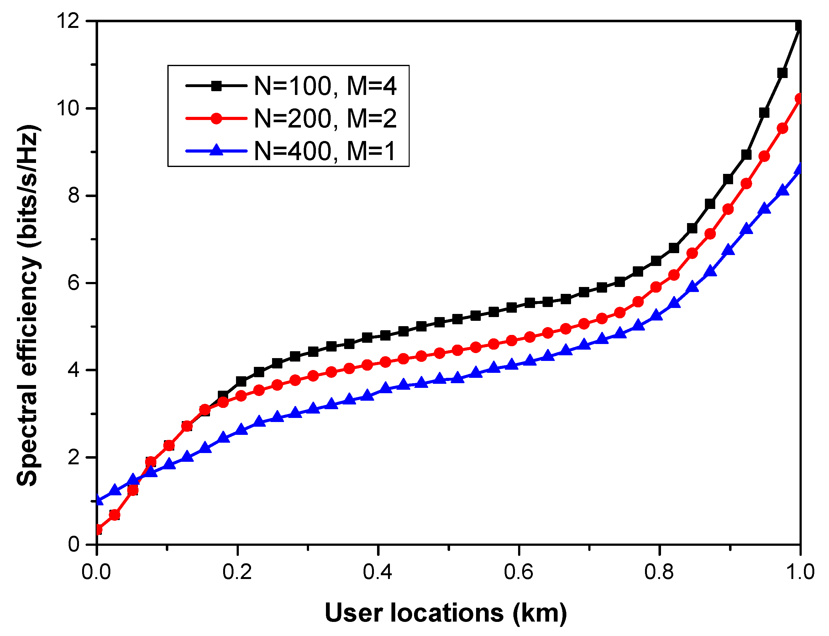
• The performance of the proposed model is evaluated through parametric variations in the number of antennas at the AP, the number of APs, and AP deployments for different network operations;
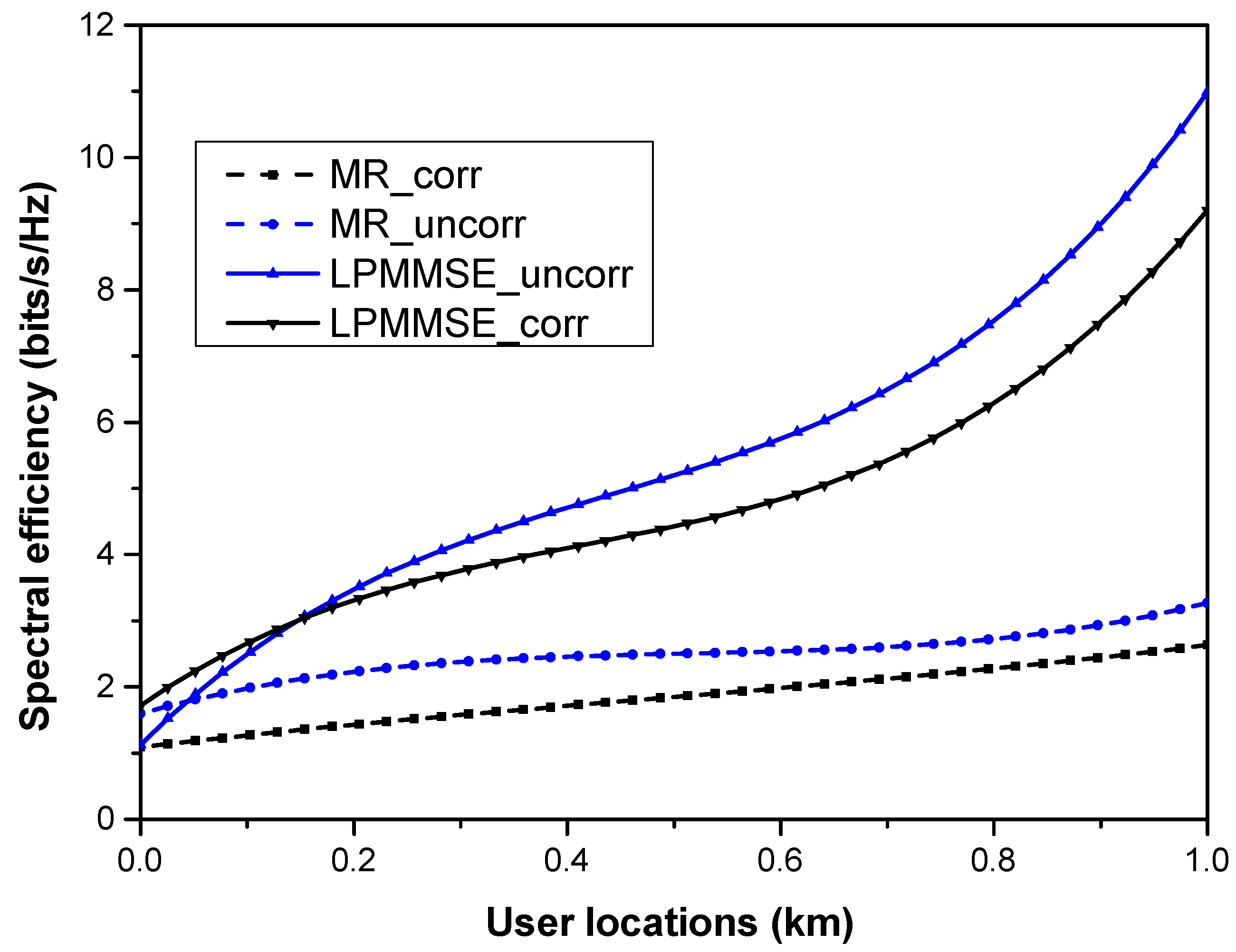
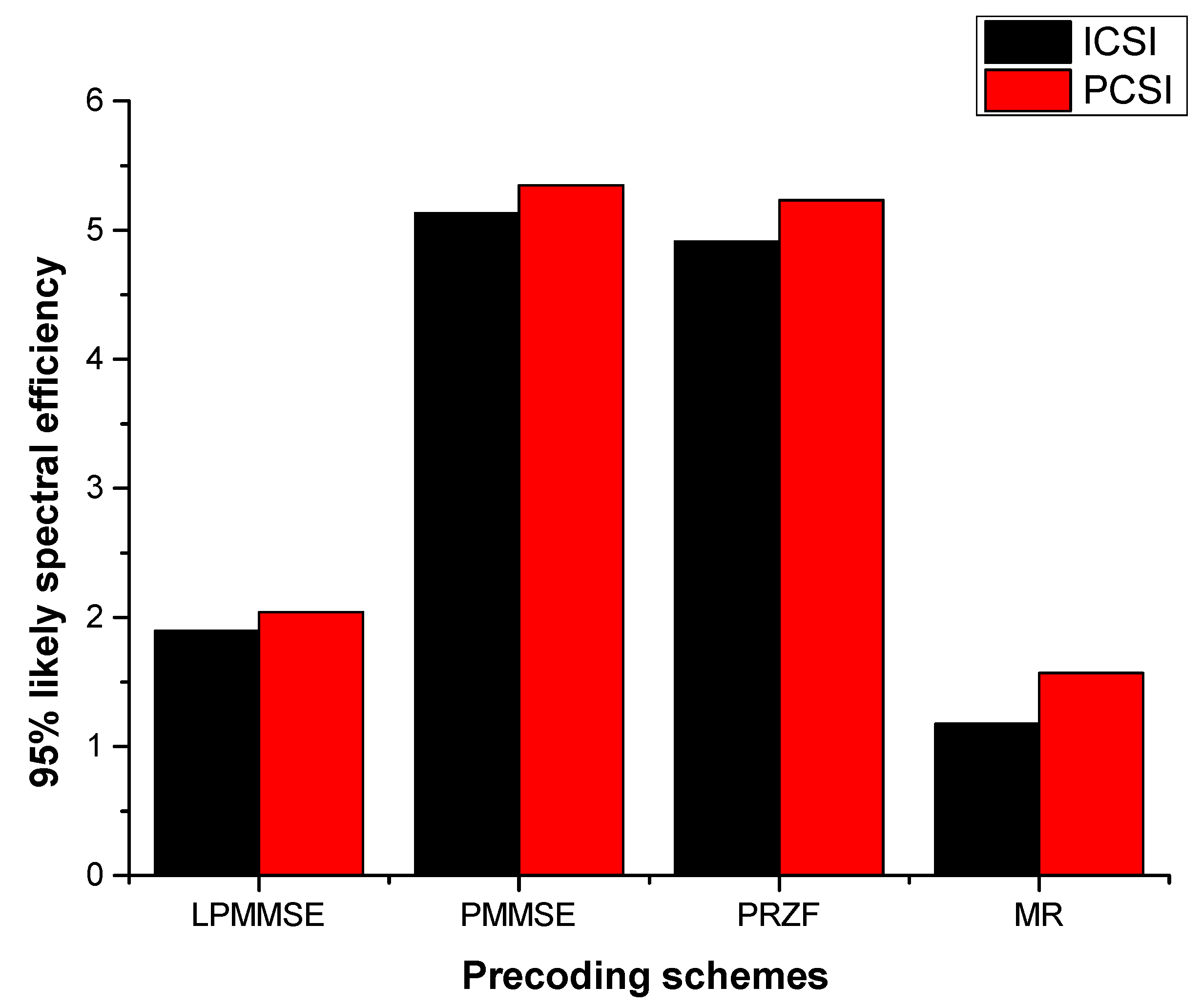
• The impact of spatial correlation and the access to perfect CSI on the network performance is also evaluated for different precoding schemes;
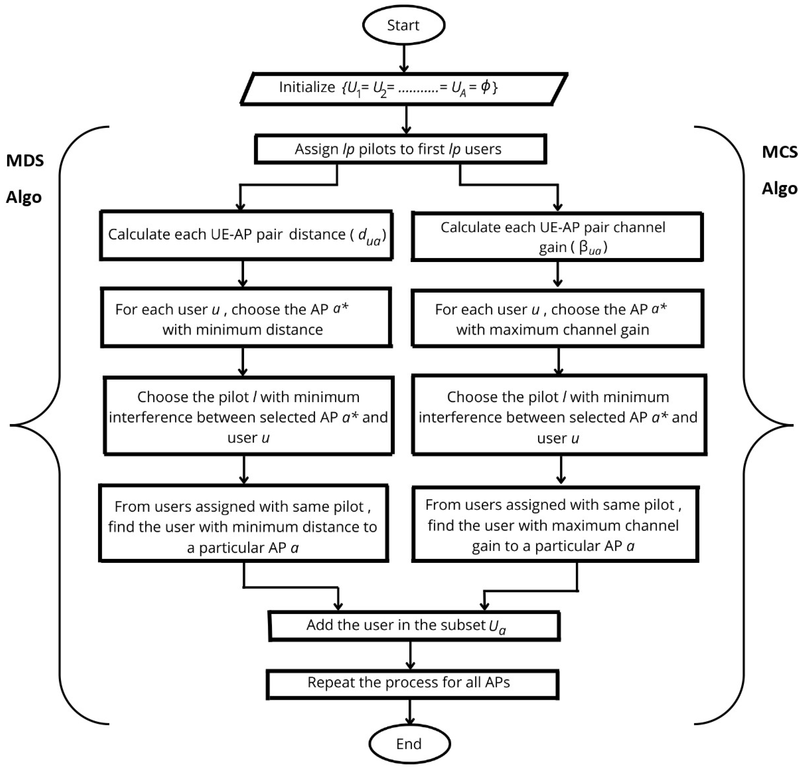
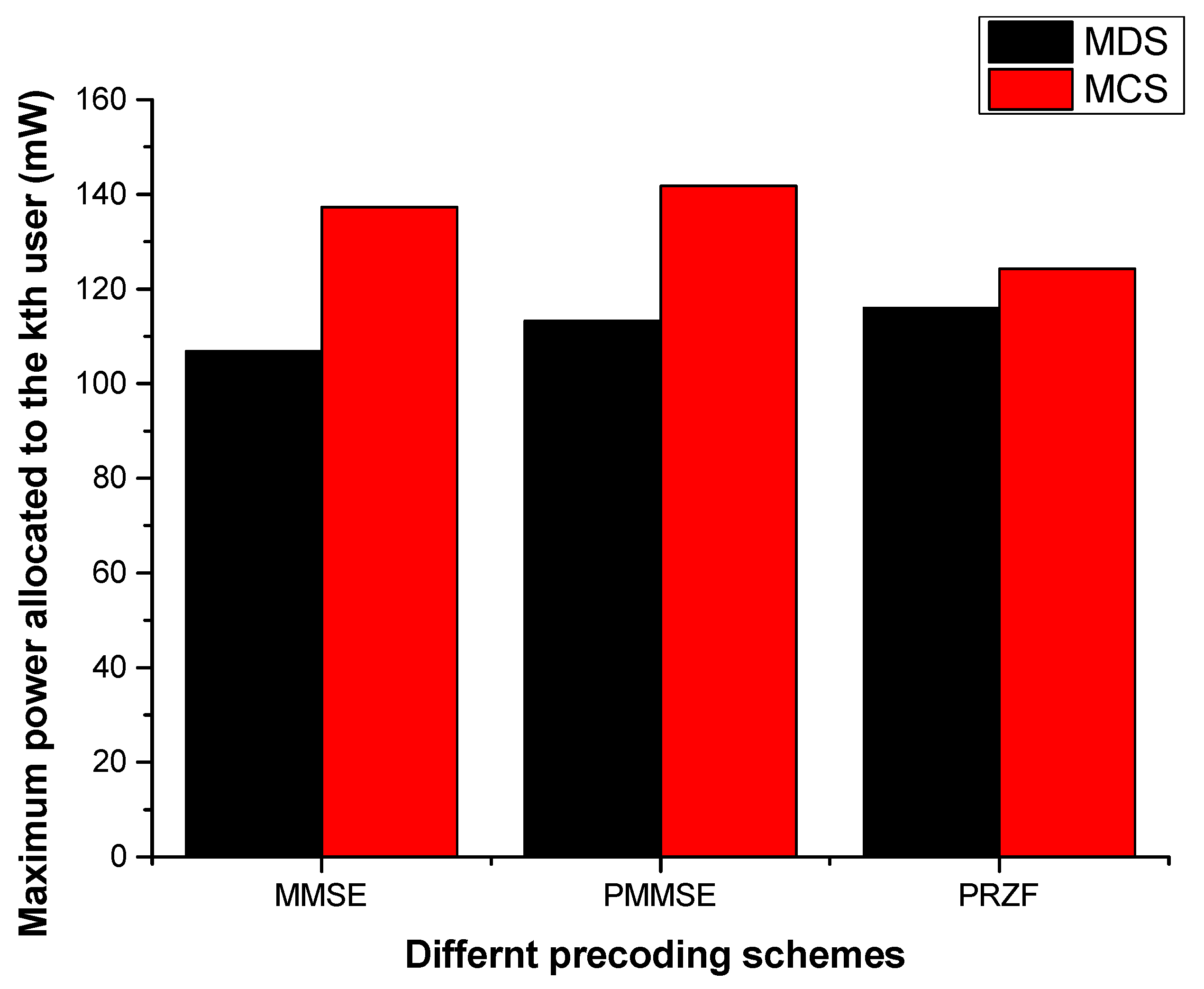
• Two user-scheduling algorithms, namely, minimum distance scheduling (MDS) and maximum channel gain scheduling (MCS), are proposed that assign a set of users to a particular AP. The minimum distance and the maximum channel gain between a user and an AP are considered for selection criteria;
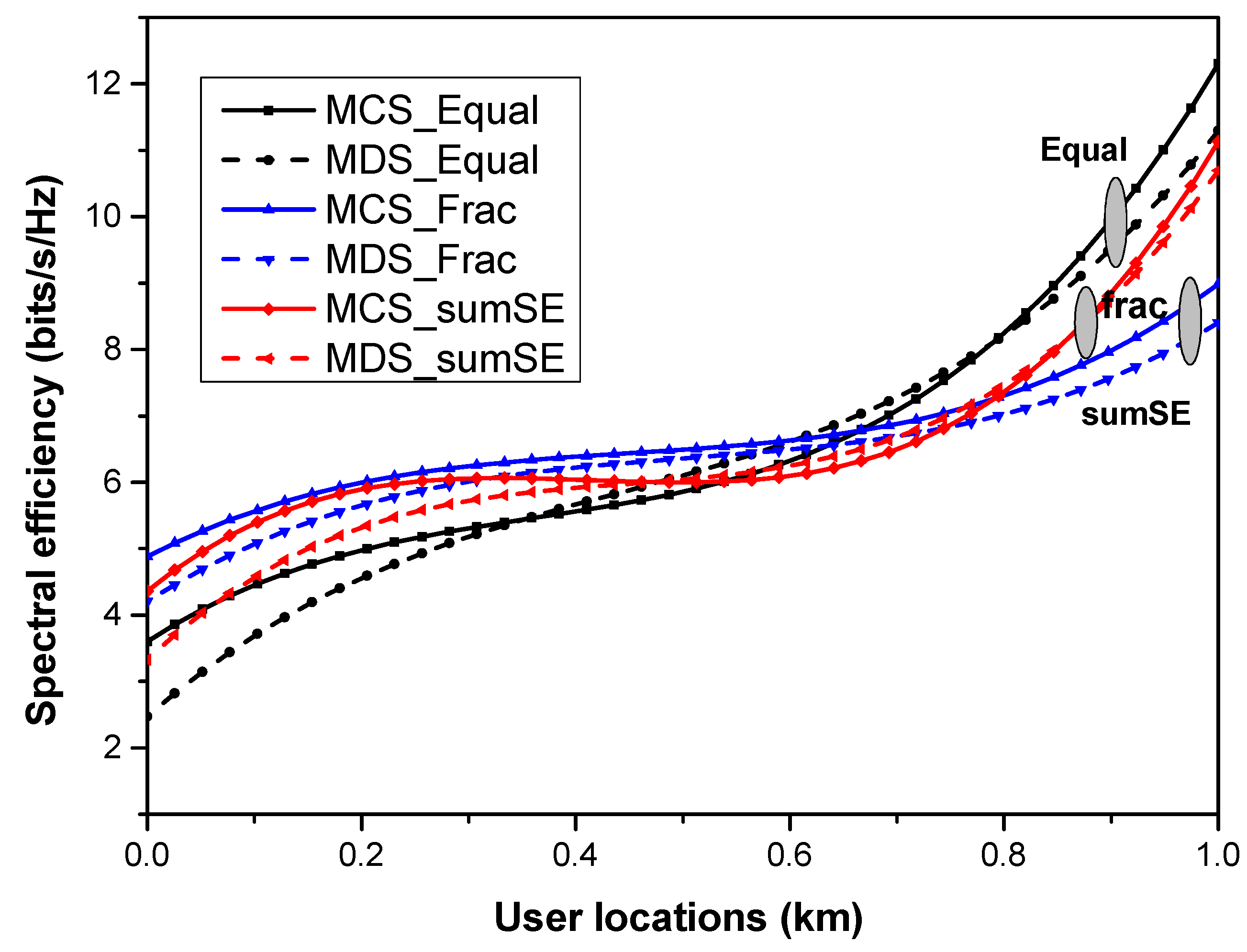
• The performance of the proposed algorithms is evaluated for three power allocation methods, namely, equal power, fractional power, and sum SE maximization power allocation mechanisms, so as to guarantee higher spectral efficiency for all the users in the network.

Figure 1 presents the communication scenario with dense AP deployment serving a large number of users.

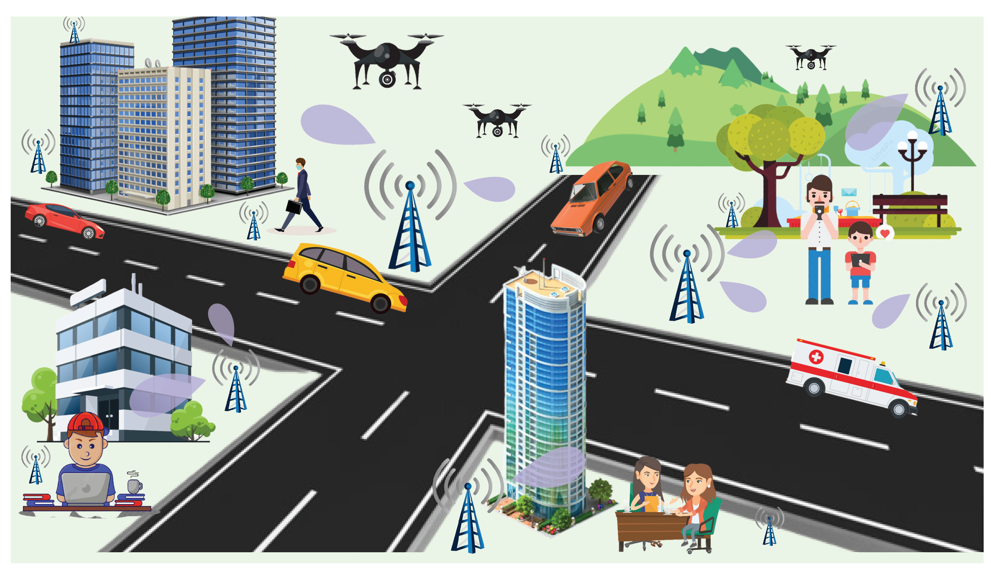
2. System Model

Consider a cell-free massive MIMO system in which a number A of APs equipped with N antennas are deployed randomly in a given geographical area. A total of U users, each with single antenna, are distributed in the given area to be served by the APs. Each AP serves a subset of users which are selected based on user needs. Each AP is connected to the CPU via fronthaul. A total of $l_p$ mutually orthogonal pilots are sent in the uplink to obtain the channel estimates. Channel reciprocity is assumed to obtain the downlink channel coefficients. The data transmission takes place in blocks of $l_c$ samples, each with coherence time $T_c$ and coherence bandwidth $B_c$. The uplink data samples in each block has length $l_u$, while the length of the downlink data is $l_d$. Correlated Rayleigh fading is considered in this paper, where a channel between AP a and user u is given as

$$h_{ua}\sim \mathcal{N}\left(0_{M,}{R}_{ua}\right),$$

(1)

$R_{ua}$ defines the spatial correlation matrix between user u and AP a. For uncorrelated channels, $R_u={\beta }_{ua}{I}_N$. In addition, $R_k=diag\left(R_{k1},\cdots \cdots R_{kN}\right)$ is the collective matrix. For finding the channel gains ${\beta }_{ua}$, a 3GPP urban microcell large-scale fading model is taken as [40]

$${\beta }_{ua}\left[dB\right]=-30.5-36.7lo{g}_{10}\left(\frac{d_{ua}}{1m}\right)+S_{kn}$$

(2)

where $S_{ua}$ denotes shadow fading and $d_{ua}$ is the distance between UE u and AP a.

2.1. Uplink Pilot Transmission

Before transmitting the uplink data signals, a set of pilots are transmitted in the uplink in order to obtain the channel estimates. A set of $l_p$ mutually orthogonal pilots signals are used to make sure that the interference from subsequent pilot transmissions is minimized. Let us suppose a subset of users that are assigned pilot l is denoted by $U_l\subset \left\{1,2,\dots \dots U\right\}$. The signal received at the ath AP from the users in the set $U_l$ is given as

$$y_{la}^p=\sum _{i\in U_l}\sqrt{l_p{p}_i}{h}_{ia}+{\mathbf{n}}_{la}$$

(3)

where ${\mathbf{n}}_{la}\sim \mathcal{N}\left(0,{\sigma }^2{I}_N\right)$ is the additive white gaussian noise and $p_i$ is the user i transmit power. The mMinimum mean square error (MMSE) estimation method is used to estimate the channel coefficients between user u and AP a [41]:

$${\widehat{h}}_{ua}=\sqrt{p_u{l}_p}{R}_{ua}{\left(\sum _{i\in U_l}{p}_i{l}_p{R}_{ia}+{\sigma }^2{I}_N\right)}^{-1}{y}_{ua}^p$$

(4)

Here, the correlation matrix of the received signal is ${\varphi }_{la}=E\left\{y_{la}^p{\left(y_{la}^p\right)}^H\right\}={\sum }_{i\in U_l}{p}_i{l}_p{R}_{ia}$ + ${\sigma }^2{I}_N$, ${\tilde{h}}_{ua}=h_{ua}-{\widehat{h}}_{ua}$, and $C_{ua}=E\left\{{\tilde{h}}_{ua}{{\tilde{h}}_{ua}}^H\right\}=R_{ua}-p_u{l}_p{R}_{ua}{\varphi }_{la}^{-1}{R}_{ua}$ is the error correlation matrix.

2.2. Uplink Data Transmission

In the uplink data transmission phase, the users transmit the data signals to the APs. Since each user is served by a subset of APs $A_u$, the data is detected using the serving APs and optimal receive combining schemes:

$${\widehat{s}}_{ua}=v_{ua}^H{G}_{ua}{y}_a^{Ul}$$

(5)

where $y_a^{Ul}={\sum }_{u=1}^U{h}_{ua}{s}_u+n_a$ is the signal received at the ath AP, $s_u$ is the signal transmitted by node u, and $n_a$ is the receiver noise. $G_{ua}$ in the uplink is given as

$$G_{ua}{v}_{ua}=\left\{\begin{array}{c}{v}_{ua}a\mathsf{ϵ}{A}_u\\ 0_{N}a\notin A_u\end{array}\right\}$$

(6)

and $G_u=diag\left(G_{u1},......G_{uA}\right)$

2.3. Downlink Data Transmission

In the downlink, the APs transmit the signals to the users. The downlink signal received at user u is

$$y_u^{Dl}=\sum _{a=1}^A{h}_{ua}^H{x}_a+n_u$$

(7)

where $n_u\sim \mathcal{N}\left(0,{\sigma }^2\right)$ is the receiver noise and $x_u$ is the signal transmitted by AP a, given as

$$x_u=\sum _{i=1}^U{G}_{ia}{w}_{ia}{\psi }_i$$

(8)

Here, $G_{ia}{w}_{ia}$ is the effective transmit precoding; it is non-zero if AP a transmits to user i. Otherwise, it will be zero.

$$G_{ia}{w}_{ia}=\left\{\begin{array}{c}{w}_{ia}aϵA_i\\ 0_{N}a\notin A_i\end{array}\right\}$$

(9)

where $A_i$ is the subset of APs that serve a user i. Equation (4) can be written equivalently as follows, by taking the summation over the user set $U_a$ served by AP a:

$$x_u=\sum _{i\in U_a}{w}_{ia}{\psi }_i$$

(10)

Thus, the received signal becomes

$$y_u^{Dl}=\sum _{i=\mathbf{1}}^U{h}_u^H{G}_i{w}_i{\psi }_i+n_u$$

(11)

where $h_u={\left[h_{u1}^T\dots \dots h_{uA}^T\right]}^T$ is the collective channel from all APs to a user u. $G_i=diag\left(G_{i1}\dots \dots G_{iA}\right)$ is the diagonal matrix which identifies which APs transmit to which user and $w_i={\left[w_{i1}^T\dots \dots w_{iA}^T\right]}^T$ is the collective precoding vector assigned to user i.

The achievable sum spectral efficiency is given by

$${SE}_u=\frac{l_d}{l_c}{log}_2\left(1+{SINR}_u\right)$$

(12)

where $SIN{R}_k$ is the signal-to-interference-plus-noise ratio achieved by the kth user, given by

$$SIN{R}_u=\frac{|E\left\{h_u^H{G}_u{w}_u\right\}{|}^{\mathbf{2}}}{{\sum }_{i=\mathbf{1}}^{K}E|h_u^H{G}_u{w}_u{|}^{\mathbf{2}}-{\left|E\left\{h_u^H{G}_u{w}_u\right\}\right|}^{\mathbf{2}}+{\sigma }^2}$$

(13)

2.4. Transmit Precoding

In the downlink of the proposed communication scenario, each AP transmits to a set of users. AP transmission to one user may cause interference to the neighboring users. Every user is affected by the interference, that is, by the data transmission to other users. Using optimal precoding schemes, it is possible that each AP can cancel out each other’s interference [42]. By adjusting the AP’s transmit powers and phases, the interference can be cancelled out [43]. This is possible in centralized operations where a CPU decides the precoding, whereas in distributed operations, each AP’s interference contribution is cancelled out using the appropriate precoding method [44]. Different transmit precodings can be used depending upon the network operation [45].

Minimum mean square error (MMSE) precoding—The centralized precoding in the downlink is the MMSE precoding, defined as

$$w_u^{MMSE}=p_u{\left(\sum _{i=\mathbf{1}}^U{p}_i{G}_u({\widehat{h}}_i{{\widehat{h}}_i}^H+C_i)G_u+{\sigma }^{\mathbf{2}}{I}_{AN}\right)}^{-1}{G}_u{\widehat{h}}_u$$

(14)

Partial minimum mean square error (PMMSE) precoding—This is an approximation to the MMSE precoding defined below:

$$w_u^{PMMSE}=p_u{\left(\sum _{i\in A_u}{p_{i}G}_u{\widehat{h}}_i{{\widehat{h}}_i}^H{G}_u+Z_{A_u}+{\sigma }^{\mathbf{2}}{I}_{AN}\right)}^{-1}{G}_u{\widehat{h}}_u$$

(15)

with $Z_{A_u}={\sum }_{i\in A_u}{p}_i{G}_u{C}_i{G}_u$

Partial regularized zero forcing (PRZF) precoding—Another low-complexity scalable precoding is PRZF precoding, which is an approximation to the MMSE precoding and is obtained as

$$w_u^{PRZF}={\left[G_u{\widehat{H}}_{A_u}{\left({\widehat{H}}_{A_u}^H{G}_u{\widehat{H}}_{A_u}+{\sigma }^2{P}_{A_u}^{-1}\right)}^{-1}\right]}_{:,1}$$

(16)

where $P_{A_u}$ is a diagonal matrix that contains the transmit powers $p_i$, and ${\widehat{H}}_{A_u}$ is a channel matrix obtained by putting together all the vectors ${\widehat{h}}_i$ for $i\in A_u$, with ${\widehat{h}}_u$ being the first column.

Local minimum mean square error (LMMSE) precoding—The locally optimal operation in the downlink is the LMMSE precoding, which includes the sum of all the users in the network and is defined as

$$w_{au}^{LMMSE}=p_u{\left(\sum _{i=\mathbf{1}}^U{p}_i({\widehat{h}}_{ia}{{\widehat{h}}_{ia}}^H+C_{ia})+{\sigma }^{\mathbf{2}}{I}_A\right)}^{-1}{G}_{ua}{\widehat{h}}_{ua}$$

(17)

Maximal ratio (MR) precoding—The MR precoding is the first scalable option; it ignores the interference caused by the AP and is obtained as

$$w_{au}^{MR}=G_{au}{\widehat{h}}_{au}$$

(18)

Local partial minimum mean square error (LPMMSE) precoding—LPMMSE precoding is a scalable approximation of the LMMSE precoding and it includes only the users served by the AP:

$$w_{au}^{LPMMSE}=p_u{\left(\sum _{i\in U_a}{p}_i({\widehat{h}}_{ia}{{\widehat{h}}_{ia}}^H+C_{ia})+{\sigma }^{\mathbf{2}}{I}_A\right)}^{-1}{G}_{ua}{\widehat{h}}_{ua}$$

(19)

3. Power Optimization

Power optimization refers to the allocation of optimal power to the users by the APs [46]. Let ${\rho }_{max}$ denote the maximum transmit power of an AP a. It is the AP that decides the power allocated to the different users depending on different parameters, such as user distances or user channel conditions. Let $\mathbf{\ae }={[{\rho }_1,{\rho }_2\dots {\rho }_U]}^T$ define the downlink power coefficients, with ${\rho }_u$ denoting the power allocated to user u by all the serving APs. The effective SINR in the downlink depends on $\mathbf{\ae }$ and can be expressed as [45]

$${\mathrm{SINR}}_u\left(\mathbf{\ae }\right)=\frac{D_u{\rho }_u}{Q_u^T\mathbf{\ae }+{\sigma }^2}$$

(20)

where

$$D_u=\frac{{\left|E\left\{h_u^H{G}_u{w}_u\right\}\right|}^2}{E\left\{\left|\right|w_u{\left|\right|}^2\right\}}\forall u$$

(21)

$$Q_{uu}=\frac{{E|h_u^H{G}_u{w}_u|}^2}{E\left\{\left|\right|w_u{\left|\right|}^2\right\}}-D_u\forall u$$

(22)

$$Q_{ui}=\frac{{E|h_u^H{G}_u{w}_i|}^2}{E\left\{\left|\right|w_i{\left|\right|}^2\right\}}\forall u,\forall i\ne u$$

(23)

Different power allocation methods are as follows:

Equal power allocation—Since each AP can serve, at most, $l_p$ users, equal power allocation assigns equal power to each user as

$${\rho }_u=\frac{{\rho }_{max}}{l_p}$$

(24)

Fractional power allocation—In this case, the power allocated to the users is proportional to the users’ channel gains to the serving APs:

$${\rho }_u={\rho }_{max}\frac{{\left({\sum }_{a\in A_u}{\beta }_{ua}\right)}^{\mu }}{{max}_{i\in A_u}{\left({\sum }_{a\in A_i}{\beta }_{ia}\right)}^{\mu }}$$

(25)

where $\mu$ is a variable that determines the power allocation behavior. Another parameter $\vartheta$ can be used to reshape the power allocation ratio between the users, known as the tuning parameter $0\le \vartheta \le 1$ [47]:

$${\rho }_u={\rho }_{max}\frac{{\left({\sum }_{a\in A_u}{\beta }_{ua}\right)}^{\mu }{\omega }_u^{-\vartheta }}{{max}_{i\in A_u}{\left({\sum }_{a\in A_i}{\beta }_{ia}\right)}^{\mu }{\omega }_i^{1-\vartheta }}$$

(26)

Sum SE maximization power allocation—Here, the optimal power to be allocated to the users is selected such that the sum of the spectral efficiencies is maximized. The sum SE maximization power allocation is represented as

$${\mathrm{maximize}}_{\rho \ge 0_{\mathrm{U}}}\sum _{\mathrm{u}=1}^{\mathrm{U}}{log}_2\left(1+\frac{{\mathrm{D}}_{\mathrm{u}}{\rho }_{\mathrm{u}}}{{\mathrm{Q}}_{\mathrm{u}}^{\mathrm{T}}\rho +{\sigma }^2}\right)$$

(27)

4. Proposed Algorithms

This section proposes two user-scheduling algorithms to select subsets of users assigned to a particular AP in the considered communication scenario. The users are selected based on two parameters: the minimum distance between a user and an AP in the MDS algorithm (minimum distance scheduling), and the maximum channel gain between a user and an AP in the MCS algorithm (maximum channel gain scheduling). The algorithms are presented in the next section along with a flowchart in Figure 2.

User-Scheduling Algorithms

In the proposed communication scenario, in a given coverage area, a large number of APs A are deployed, and each AP serves a subset of users $U_a$ from the total number of U users distributed randomly in the network. Let $\left\{U_1,U_2,.....U_A\right\}$ be the subsets of users assigned to the APs $\left\{1,2,.....A\right\}$. $l_p$ denotes the length of the mutually orthogonal pilot sequences. Initially, the pilots are assigned to the first $l_p$ users. For the remaining users, pilot assignment involves, first, choosing an AP $a^{\ast }$. In the MDS algorithm (Algo Algorithm 1), the distance between each UE–AP pair is calculated, and for a particular user u, the AP with the minimum distance to user u is selected as $a^{\ast }$. In the MCS algorithm (Algo Algorithm 2), the AP with the maximum channel gain to user u is selected as $a^{\ast }$. After that, the pilot l with minimum interference between the selected AP $a^{\ast }$ and the user u is chosen and assigned to it. In the end, for all deployed APs, users are selected. For each AP a, $l_p$ users are selected, each assigned with a different orthogonal pilot. From the users assigned with the same pilot l, the user u nearest to the AP a is selected, that is, the one with the minimum distance in the case of the MDS algorithm. In the case of the MCS algorithm, however, a user u with the maximum channel gain between u and AP a is selected. The process is repeated till the user subsets for all the APs are selected.

Algorithm 1 MDS algorithm.

Input: A, $l_p$, U Output: $U_a$, $a\in \left\{1,\dots \dots A\right\}$ Initialization: $\left\{U_1=U_2=\dots \dots =U_A=\varphi \right\}$ while$u<l_p$ $l_u\leftarrow u$ while$u>l_p$ find $a^{\ast }$ $a^{\ast }\leftarrow {argmin}_{a\in \left\{1,\dots \dots A\right\}}{d}_{ua}$ find $l^{\prime }$ $l^{\prime }\leftarrow {argmin}_{l\in \left\{1,\dots \dots ,l_p\right\}}{\sum }_{i=1,l_i=l}^{u-1}{\beta }_{i{a}^{\ast }}$ $l_u\leftarrow l^{\prime }$ fora=1:A forl=1:$l_p$ $i\leftarrow {argmin}_{u\in \left\{1,\dots \dots U\right\},l_u=l}{d}_{ua}$ $U_i=U_i\cup \left\{u\right\}$ return$U_i$

Algorithm 2 MCS algorithm.

Input: A, $l_p$, U Output: $U_a$, $a\in \left\{1,\dots \dots A\right\}$ Initialization: $\left\{U_1=U_2=\dots \dots =U_A=\varphi \right\}$ while$u<l_p$ $l_u\leftarrow u$ while$u>l_p$ find $a^{\ast }$ $a^{\ast }\leftarrow {argmax}_{a\in \left\{1,\dots \dots A\right\}}{\beta }_{ua}$ find $l^{\prime }$ $l^{\prime }\leftarrow {argmin}_{l\in \left\{1\dots \dots ,l_p\right\}}{\sum }_{i=1,l_i=l}^{u-1}{\beta }_{i{a}^{\ast }}$ $l_u\leftarrow l^{\prime }$ fora=1:A forl=1:$l_p$ $i\leftarrow {argmax}_{k\in \left\{1,\dots \dots K\right\},l_u=l}{\beta }_{ua}$ $U_i=U_i\cup \left\{u\right\}$ return$U_i$

5. Results and Discussion

The paper evaluates the performance of the proposed model with a power-control mechanism. It enables the selection of optimal power coefficients such that the system performance is improved. The network scenario is simulated in MATLAB, taking ${10}^4$ iterations per simulation setup. The network coverage area of 1 Km × 1 Km is considered in, which 100–400 access points (APs) are deployed at random. The user distribution is taken to be uniform within the coverage area. The system is simulated for different parametric variations with different power optimization mechanisms, precoding schemes, spatial correlations, and CSI availabilities. A comparison of the two proposed algorithms based on minimum distance and maximum channel gain is also carried out. The results are presented and explained in this section. Important parameters for simulation are considered in

Table 1. Important parameters considered in the simulation setup.

Parameters	Value	Parameters	Value
U	40	$l_p$	10
A	100	$l_c$	200
N	4	$p_u$	100 mW
B	20 MHz	${\sigma }^2$	$-94$ dBm
$T_c$	2 ms	${\rho }_{max}$	200 mW
$B_c$	100 kHz	$h^{\prime }$	10 m
$\alpha$	3.76

.

The communication framework proposed in the paper is first evaluated for different deployments of APs in the coverage area. The APs are densely deployed in the given area to provide extended coverage to the users. It has been shown in Figure 3 that more densely deployed single-antenna APs see a drop in spectral efficiency for all user locations, except in the lower region. With more number of antennas at the APs, the spectral efficiency improves even if the deployment of APs is less dense. The performance evaluation is carried out using the LMMSE precoding scheme, which leads to better interference suppression with M = 4, resulting in improved SE performance.

The distributed network operation with the MR and LPMMSE precoding methods is shown in Figure 4. The effect of spatial correlation on the performance of the network is evaluated. With spatially correlated Rayleigh fading channels, the SE degrades with both MR and LPMMSE precoding schemes. Since all the signal processing is carried out locally at the AP, this network operation could not exploit the spatial correlation. Additionally, the system with highly correlated channels has less average spectral efficiency (SE), as compared to the system with lower spatial correlation.

The availability of knowledge of the channel state information (CSI) plays an important role in determining the performance of any wireless network. This is depicted in Figure 5 for the centralized and distributed precoding schemes, namely, PMMSE, PRZF, LPMMSE, and MR. The achieved SE by $95\%$ of the users in the network area is plotted for the different precoding schemes under two cases. In the first case, it is assumed that users have access to the perfect channel state information (PCSI), while the second case considers channel estimates for data detection, that is, imperfect CSI (ICSI). The maximum value of 5.3462 bits/s/Hz is achieved with PMMSE precoding with PCSI, while the least SE of 1.1745 bits/s/Hz is achieved with MR precoding with the IMCSI case. There is an improvement of $4.1\%$ in the achieved SE with PMMSE precoding with PCSI, compared to the ICSI case.

The performance of the system with power optimization mechanisms is evaluated further. Power optimization refers to the selection of optimum power with which a particular AP transmits to a particular user such that the system efficiency is increased. Three power-allocation mechanisms are considered in this paper, namely, equal power allocation, fractional power allocation, and sum spectral efficiency maximization power allocation. The maximum power allocated to the kth user under fractional power allocation is plotted for different precoding schemes in Figure 6 using the proposed algorithms. It is observed that maximum power is allocated to the users with the MCS algorithm, compared to the MDS algorithm. Depending upon the user distances and channel gains, each AP with a maximum transmit power of 200 mW allocates different powers to different users. Using centralized PMMSE precoding, each AP assigns a maximum power of 141.7 mW to a user with strong channel conditions with the AP and a minimum power of 3.1882 mW to the user with the worst channel conditions. Figure 7 gives a comparison of the spectral efficiency achieved by the three power-allocation methods under the proposed algorithms. As compared to MDS algorithm, the MCS algorithm results in better spectral efficiency for all the users. This is because the latter considers the users’ channel gains as the selection criteria. Equal power allocation results in improved SE in the upper region, while sum SE power allocation is recommended in the lower region. The optimum performance is achieved with the fractional power allocation with which most of the users attain higher SE.

Table 2. Power allocated to the users with the fractional power mechanism for different precoding schemes.

Precoding Scheme	$\mathit{\mu }$ = 0.5, $\mathit{\vartheta }$ = 1	$\mathit{\mu }$ = 0.5, $\mathit{\vartheta }$ = 0.5	$\mathit{\mu }$ = −0.5, $\mathit{\vartheta }$ = 1	$\mathit{\mu }$ = −0.5, $\mathit{\vartheta }$ = 0.5	$\mathit{\mu }$ = −0.5, $\mathit{\vartheta }$ = 0
MMSE (max)	58.2182	119.1856	154.4216	137.3216	81.6737
MMSE (min)	3.1003	2.0158	1.5627	3.1524	1.6351
PMMSE (max)	58.2706	119.9334	159.6505	141.7682	84.2957
PMMSE (min)	3.1708	2.1165	1.5590	3.1882	1.6602
PRZF (max)	58.8072	121.3019	183.0052	124.2476	95.2498
PRZF(min)	3.4914	2.3629	1.6656	3.3612	1.8452

gives the maximum and minimum power values allocated to the users under different precoding schemes for different values of FPA parameters. It has been observed that the power allocated to the users varies with the precoding schemes and the FPA parameters. With MMSE precoding, a user is assigned a maximum power of 154.42 mW and a minimum power of 1.5627 mW for $\mu$ = −0.5 and $\vartheta$ = 1. With PRZF precoding, these values are 159.65 mW and 1.5590 mW, respectively. Moreover, PMMSE precoding with the same FPA parameters ($\mu$ = −0.5 and $\vartheta$ = 1) assigns a maximum power of 154.42 mW and a minimum power of 1.5590 mW.

6. Conclusions

A massive IoT network involves information flow between a massive number of connected devices for varied IoT application verticals. The high power consumption and huge energy overhead are the main challenges of this digital network powered by battery-limited devices. Thus, the network service providers are looking for sustainable energy solutions to meet the energy demands of these networks. This paper presents a practical power-allocation model that optimizes the power resources, resulting in increased network efficiency. Two user-scheduling algorithms are proposed which select a set of users to be served by each AP. The performance of the proposed model is evaluated through parametric variations in the number of antennas at the AP, AP deployment, CSI availability, and spatial correlation for different precoding schemes. It is observed that less densely deployed APs with multiple antennas yield more spectral efficiency. In the distributed network operation where all the signal processing occurs at the AP, the network performance degrades with spatial correlation for both MR and LPMMSE precoding. The availability of perfect CSI suggests an improvement of $4.1\%$ in the achieved SE by $95\%$ of the users in the network with PMMSE precoding. Further, the performance of the system with power optimization mechanisms are carried out with the two proposed user-scheduling algorithms. Using centralized PMMSE precoding, each AP assigns a maximum power of 141.7 mW to a user with a strong channel and a minimum power of 3.1882 mW to the user with the weakest channel, with fractional power allocation for $\mu$ = −0.5, $\vartheta$ = 0.5. As compared to the MDS algorithm, the MCS algorithm results in better spectral efficiency for all the users. Optimum performance is also achieved with the fractional power allocation, with which most of the users attain higher SE.

References

- Mao, B.; Tang, F.; Kawamoto, Y.; Kato, N. AI Models for Green Communications Towards 6G. IEEE Commun. Surv. Tutor. 2022, 24, 210–247. [Google Scholar] [CrossRef]
- Verma, S.; Kaur, S.; Khan, M.A.; Sehdev, P.S. Toward Green Communication in 6G-Enabled Massive Internet of Things. IEEE Internet Things J. 2021, 8, 5408–5415. [Google Scholar] [CrossRef]
- Wang, J.; Zhu, K.; Hossain, E. Green Internet of Vehicles (IoV) in the 6G Era: Toward Sustainable Vehicular Communications and Networking. IEEE Trans. Green Commun. Netw. 2022, 6, 391–423. [Google Scholar] [CrossRef]
- Huang, T.; Yang, W.; Wu, J.; Ma, J.; Zhang, X.; Zhang, D. A Survey on Green 6G Network: Architecture and Technologies. IEEE Access 2019, 7, 175758–175768. [Google Scholar] [CrossRef]
- Moya Osorio, D.P.; Ahmad, I.; Sánchez, J.D.V.; Gurtov, A.; Scholliers, J.; Kutila, M.; Porambage, P. Towards 6G-Enabled Internet of Vehicles: Security and Privacy. IEEE Open J. Commun. Soc. 2022, 3, 82–105. [Google Scholar] [CrossRef]
- Nekovee, M. Transformation from 5G for Verticals Towards a 6G-enabled Internet of Verticals. In Proceedings of the 2022 14th International Conference on COMmunication Systems NETworkS (COMSNETS), Bangalore, India, 4–8 January 2022; pp. 1–6. [Google Scholar] [CrossRef]
- Vaezi, M.; Azari, A.; Khosravirad, S.R.; Shirvanimoghaddam, M.; Azari, M.M.; Chasaki, D.; Popovski, P. Cellular, Wide-Area, and Non-Terrestrial IoT: A Survey on 5G Advances and the Road Towards 6G. IEEE Commun. Surv. Tutor. 2022, 24, 1117–1174. [Google Scholar] [CrossRef]
- Zhang, Q.; Yang, H.H.; Quek, T.Q.S.; Lee, J. Heterogeneous Cellular Networks With LoS and NLoS Transmissions—The Role of Massive MIMO and Small Cells. IEEE Trans. Wirel. Commun. 2017, 16, 7996–8010. [Google Scholar] [CrossRef] [Green Version]
- Björnson, E.; Sanguinetti, L.; Wymeersch, H.; Hoydis, J.; Marzetta, T.L. Massive MIMO is a reality—What is next?: Five promising research directions for antenna arrays. Digit. Signal Process. 2019, 94, 3–20. [Google Scholar] [CrossRef]
- Jain, I.K.; Kumar, R.; Panwar, S.S. The Impact of Mobile Blockers on Millimeter Wave Cellular Systems. IEEE J. Sel. Areas Commun. 2019, 37, 854–868. [Google Scholar] [CrossRef] [Green Version]
- Zhang, J.; Dai, L.; Li, X.; Liu, Y.; Hanzo, L. On Low-Resolution ADCs in Practical 5G Millimeter-Wave Massive MIMO Systems. IEEE Commun. Mag. 2018, 56, 205–211. [Google Scholar] [CrossRef] [Green Version]
- Pang, X.; Zhao, N.; Tang, J.; Wu, C.; Niyato, D.; Wong, K.K. IRS-Assisted Secure UAV Transmission via Joint Trajectory and Beamforming Design. IEEE Trans. Commun. 2022, 70, 1140–1152. [Google Scholar] [CrossRef]
- Taneja, A.; Rani, S.; Alhudhaif, A.; Koundal, D.; Gündüz, E.S. An optimized scheme for energy efficient wireless communication via intelligent reflecting surfaces. Expert Syst. Appl. 2022, 190, 116106. [Google Scholar] [CrossRef]
- Zhang, J.; Chen, S.; Lin, Y.; Zheng, J.; Ai, B.; Hanzo, L. Cell-Free Massive MIMO: A New Next-Generation Paradigm. IEEE Access 2019, 7, 99878–99888. [Google Scholar] [CrossRef]
- Buzzi, S.; D’Andrea, C.; Zappone, A.; D’Elia, C. User-Centric 5G Cellular Networks: Resource Allocation and Comparison with the Cell-Free Massive MIMO Approach. IEEE Trans. Wirel. Commun. 2020, 19, 1250–1264. [Google Scholar] [CrossRef] [Green Version]
- Ammar, H.A.; Adve, R.; Shahbazpanahi, S.; Boudreau, G.; Srinivas, K.V. User-Centric Cell-Free Massive MIMO Networks: A Survey of Opportunities, Challenges and Solutions. IEEE Commun. Surv. Tutor. 2022, 24, 611–652. [Google Scholar] [CrossRef]
- Balachandran, K.; Kang, J.H.; Karakayali, K.M.; Rege, K.M. Network-centric cooperation schemes for uplink interference management in cellular networks. Bell Labs Tech. J. 2013, 18, 23–36. [Google Scholar] [CrossRef]
- Peng, M.; Sun, Y.; Li, X.; Mao, Z.; Wang, C. Recent Advances in Cloud Radio Access Networks: System Architectures, Key Techniques, and Open Issues. IEEE Commun. Surv. Tutor. 2016, 18, 2282–2308. [Google Scholar] [CrossRef] [Green Version]
- Björnson, E.; Sanguinetti, L. A New Look at Cell-Free Massive MIMO: Making It Practical With Dynamic Cooperation. In Proceedings of the 2019 IEEE 30th Annual International Symposium on Personal, Indoor and Mobile Radio Communications (PIMRC), Istanbul, Turkey, 8–11 September 2019; pp. 1–6. [Google Scholar] [CrossRef] [Green Version]
- Interdonato, G.; Karlsson, M.; Björnson, E.; Larsson, E.G. Local Partial Zero-Forcing Precoding for Cell-Free Massive MIMO. IEEE Trans. Wirel. Commun. 2020, 19, 4758–4774. [Google Scholar] [CrossRef] [Green Version]
- Attarifar, M.; Abbasfar, A.; Lozano, A. Modified Conjugate Beamforming for Cell-Free Massive MIMO. IEEE Wirel. Commun. Lett. 2019, 8, 616–619. [Google Scholar] [CrossRef] [Green Version]
- Yan, H.; Ashikhmin, A.; Yang, H. A Scalable and Energy-Efficient IoT System Supported by Cell-Free Massive MIMO. IEEE Internet Things J. 2021, 8, 14705–14718. [Google Scholar] [CrossRef]
- Björnson, E.; Sanguinetti, L. Making Cell-Free Massive MIMO Competitive With MMSE Processing and Centralized Implementation. IEEE Trans. Wirel. Commun. 2020, 19, 77–90. [Google Scholar] [CrossRef] [Green Version]
- Sanguinetti, L.; Björnson, E.; Hoydis, J. Toward Massive MIMO 2.0: Understanding Spatial Correlation, Interference Suppression, and Pilot Contamination. IEEE Trans. Commun. 2020, 68, 232–257. [Google Scholar] [CrossRef] [Green Version]
- Ngo, H.Q.; Ashikhmin, A.; Yang, H.; Larsson, E.G.; Marzetta, T.L. Cell-Free Massive MIMO Versus Small Cells. IEEE Trans. Wirel. Commun. 2017, 16, 1834–1850. [Google Scholar] [CrossRef] [Green Version]
- Mai, T.C.; Ngo, H.Q.; Duong, T.Q. Downlink Spectral Efficiency of Cell-Free Massive MIMO Systems With Multi-Antenna Users. IEEE Trans. Commun. 2020, 68, 4803–4815. [Google Scholar] [CrossRef]
- Burr, A.; Islam, S.; Zhao, J.; Bashar, M. Cell-free Massive MIMO with multi-antenna access points and user terminals. In Proceedings of the 2020 54th Asilomar Conference on Signals, Systems, and Computers, Pacific Grove, CA, USA, 1–4 November 2020; pp. 821–825. [Google Scholar] [CrossRef]
- Mai, T.C.; Quoc Ngo, H.; Duong, T.Q. Cell-free massive mimo systems with multi-antenna users. In Proceedings of the 2018 IEEE Global Conference on Signal and Information Processing (GlobalSIP), Anaheim, CA, USA, 26–29 November 2018; pp. 828–832. [Google Scholar] [CrossRef]
- López, O.L.A.; Alves, H.; Souza, R.D.; Montejo-Sánchez, S.; Fernández, E.M.G.; Latva-Aho, M. Massive Wireless Energy Transfer: Enabling Sustainable IoT Toward 6G Era. IEEE Internet Things J. 2021, 8, 8816–8835. [Google Scholar] [CrossRef]
- Izadi, A.; Razavizadeh, S.M.; Saatlou, O. Power Allocation for Downlink Training in Cell-Free Massive MIMO Networks. In Proceedings of the 2020 10th International Symposium onTelecommunications (IST), Tehran, Iran, 15–17 December 2020; pp. 111–115. [Google Scholar] [CrossRef]
- Chakraborty, S.; Demir, Ö.T.; Björnson, E.; Giselsson, P. Efficient Downlink Power Allocation Algorithms for Cell-Free Massive MIMO Systems. IEEE Open J. Commun. Soc. 2021, 2, 168–186. [Google Scholar] [CrossRef]
- Van Chien, T.; Björnson, E.; Larsson, E.G. Joint Power Allocation and Load Balancing Optimization for Energy-Efficient Cell-Free Massive MIMO Networks. IEEE Trans. Wirel. Commun. 2020, 19, 6798–6812. [Google Scholar] [CrossRef]
- Guenach, M.; Gorji, A.A.; Bourdoux, A. Joint Power Control and Access Point Scheduling in Fronthaul-Constrained Uplink Cell-Free Massive MIMO Systems. IEEE Trans. Commun. 2021, 69, 2709–2722. [Google Scholar] [CrossRef]
- Yang, H.; Marzetta, T.L. Energy Efficiency of Massive MIMO: Cell-Free vs. Cellular. In Proceedings of the 2018 IEEE 87th Vehicular Technology Conference (VTC Spring), Porto, Portugal, 3–6 June 2018; pp. 1–5. [Google Scholar] [CrossRef]
- Ngo, H.Q.; Tran, L.N.; Duong, T.Q.; Matthaiou, M.; Larsson, E.G. On the Total Energy Efficiency of Cell-Free Massive MIMO. IEEE Trans. Green Commun. Netw. 2018, 2, 25–39. [Google Scholar] [CrossRef] [Green Version]
- Chen, S.; Zhang, J.; Jin, Y.; Ai, B. Wireless powered IoE for 6G: Massive access meets scalable cell-free massive MIMO. China Commun. 2020, 17, 92–109. [Google Scholar] [CrossRef]
- Clerckx, B.; Huang, K.; Varshney, L.R.; Ulukus, S.; Alouini, M.S. Wireless Power Transfer for Future Networks: Signal Processing, Machine Learning, Computing, and Sensing. IEEE J. Sel. Top. Signal Process. 2021, 15, 1060–1094. [Google Scholar] [CrossRef]
- Demir, Ö.T.; Björnson, E. Joint Power Control and LSFD for Wireless-Powered Cell-Free Massive MIMO. IEEE Trans. Wirel. Commun. 2021, 20, 1756–1769. [Google Scholar] [CrossRef]
- Zhang, Y.; Xia, W.; Zhao, H.; Xu, W.; Wong, K.K.; Yang, L. Cell-Free IoT Networks with SWIPT: Performance Analysis and Power Control. IEEE Internet Things J. 2022. [Google Scholar] [CrossRef]
- 3GPP. Further Advancements for E-UTRA Physical Layer Aspects (Release 9). In 3GPP Technical Specification 36.814; 3GPP: Valbonne, France, 2017. [Google Scholar]
- Björnson, E.; Hoydis, J.; Sanguinetti, L. Massive MIMO networks: Spectral, energy, and hardware efficiency. Found. Trends Signal Process. 2017, 11, 154–655. [Google Scholar] [CrossRef]
- Taneja, A.; Saluja, N. Linear precoding with user and transmit antenna selection. Wirel. Pers. Commun. 2019, 109, 1631–1644. [Google Scholar] [CrossRef]
- Palhares, V.M.T.; Flores, A.R.; de Lamare, R.C. Robust MMSE Precoding and Power Allocation for Cell-Free Massive MIMO Systems. IEEE Trans. Veh. Technol. 2021, 70, 5115–5120. [Google Scholar] [CrossRef]
- Atzeni, I.; Gouda, B.; Tölli, A. Distributed Precoding Design via Over-the-Air Signaling for Cell-Free Massive MIMO. IEEE Trans. Wirel. Commun. 2021, 20, 1201–1216. [Google Scholar] [CrossRef]
- Nayebi, E.; Ashikhmin, A.; Marzetta, T.L.; Yang, H.; Rao, B.D. Precoding and Power Optimization in Cell-Free Massive MIMO Systems. IEEE Trans. Wirel. Commun. 2017, 16, 4445–4459. [Google Scholar] [CrossRef]
- Tripathi, S.C.; Trivedi, A.; Rajoria, S. Power Optimization of Cell Free massive MIMO with Zero-forcing Beamforming Technique. In Proceedings of the 2018 Conference on Information and Communication Technology (CICT), Jabalpur, India, 26–28 October 2018; pp. 1–4. [Google Scholar] [CrossRef]
- Nikbakht, R.; Mosayebi, R.; Lozano, A. Uplink Fractional Power Control and Downlink Power Allocation for Cell-Free Networks. IEEE Wirel. Commun. Lett. 2020, 9, 774–777. [Google Scholar] [CrossRef]