
Wind Power Forecasting Based on LSTM Improved by EMD-PCA-RF

Abstract
:1. Introduction
2. Methods
2.1. LASSO Algorithm
2.2. EMD Algorithm
2.3. PCA-RF Combined Algorithm
2.3.1. PCA Algorithm
2.3.2. RF Algorithm
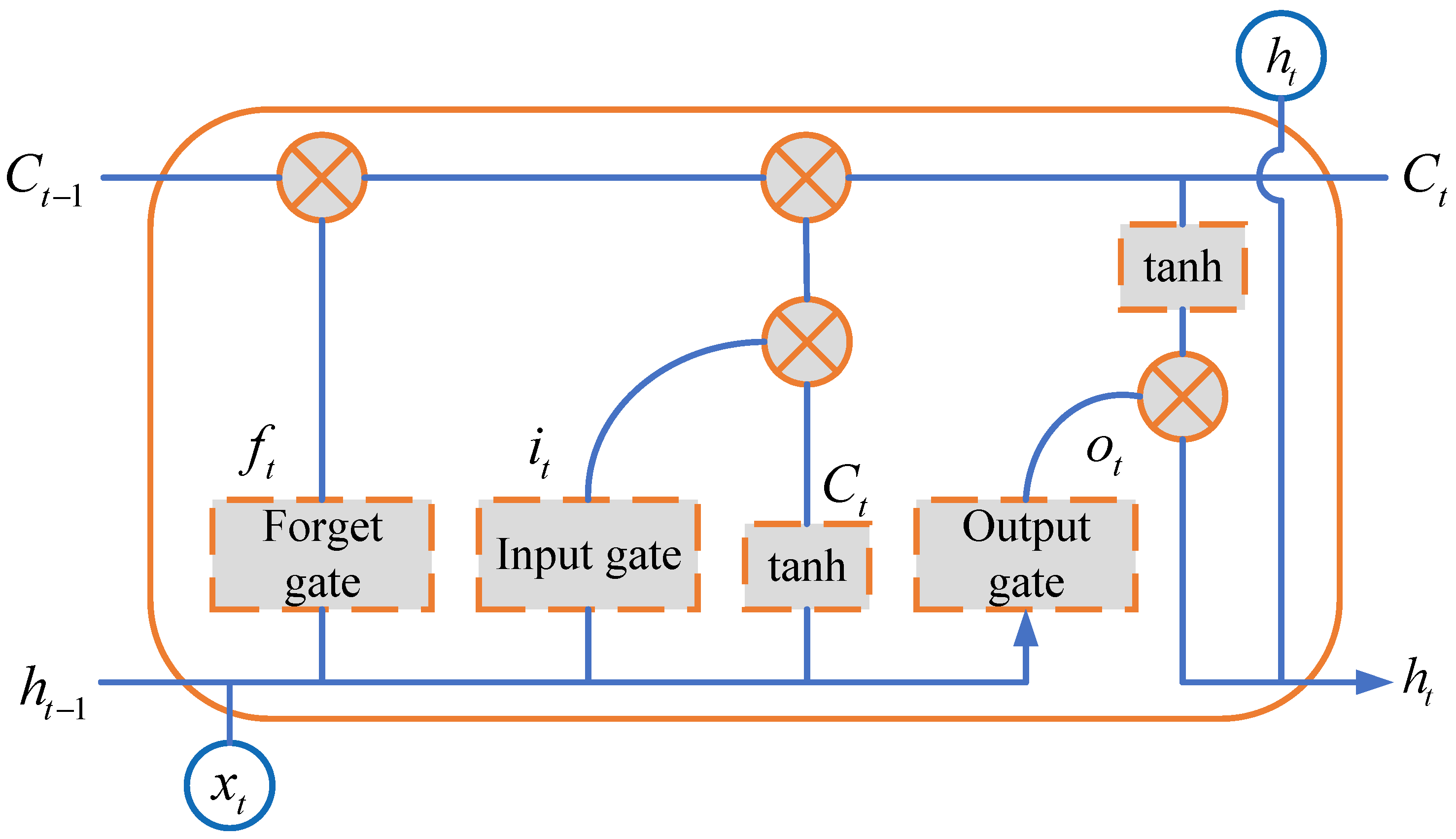
2.4. LSTM Algorithm
3. Data Pre-Processing and Model Design
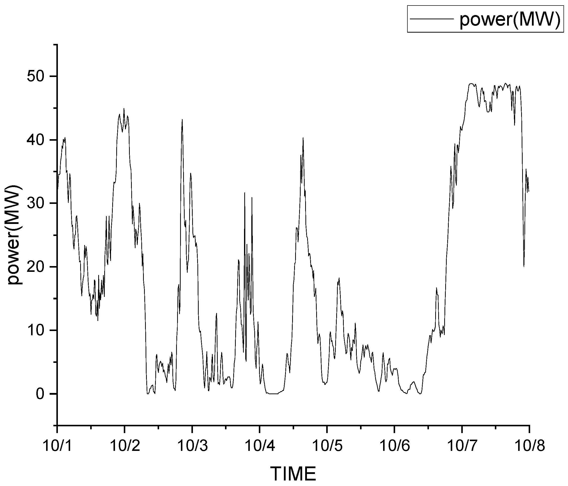
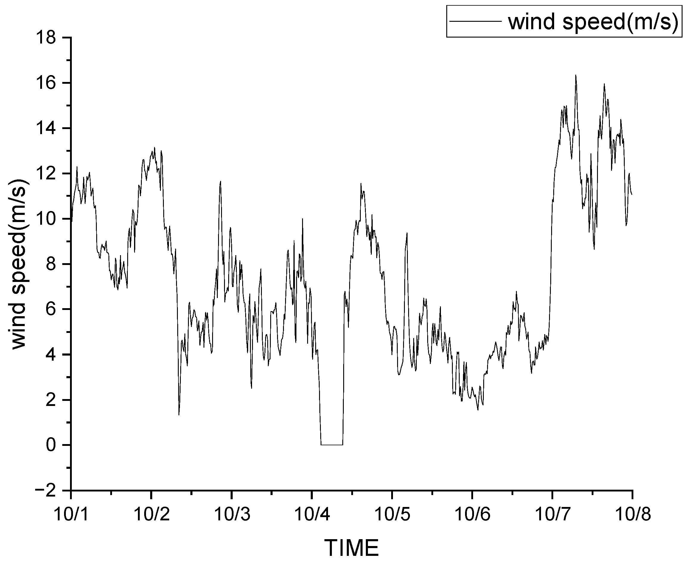
3.1. Data Sources
3.2. Environmental Factors Selection Based on LASSO
3.3. Construction of Wind Power Forecasting Model
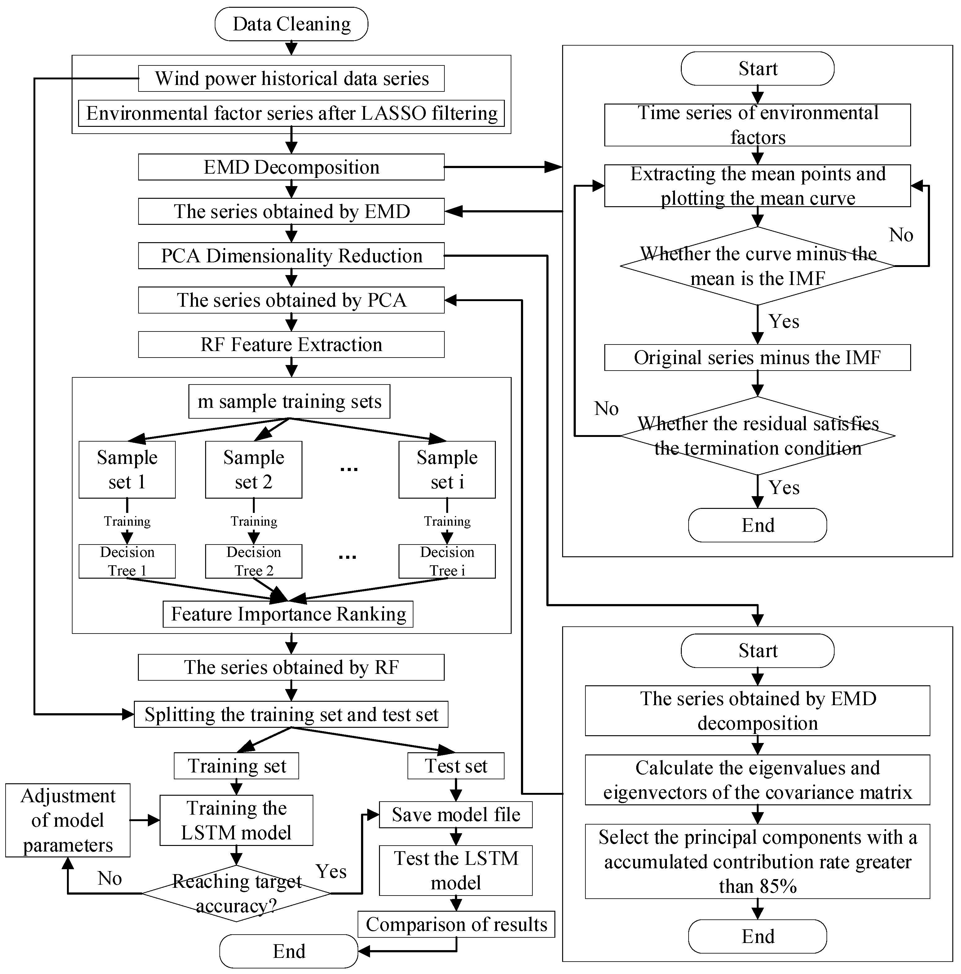
3.3.1. Wind Power Forecasting Model Based on EMD-PCA-RF-LSTM
| Algorithm 1: EMD-PCA-RF-LSTM-based wind power forecasting algorithm. |
| Input: DATE, humidity, temp, pressure, wind_dir, wind_speed, power |
| Output: Forecasting results, model evaluation indicators (MSE, RMSE, MAE, R2/adj-R2). |
|
3.3.2. Model Evaluation Indicators
4. Case Study
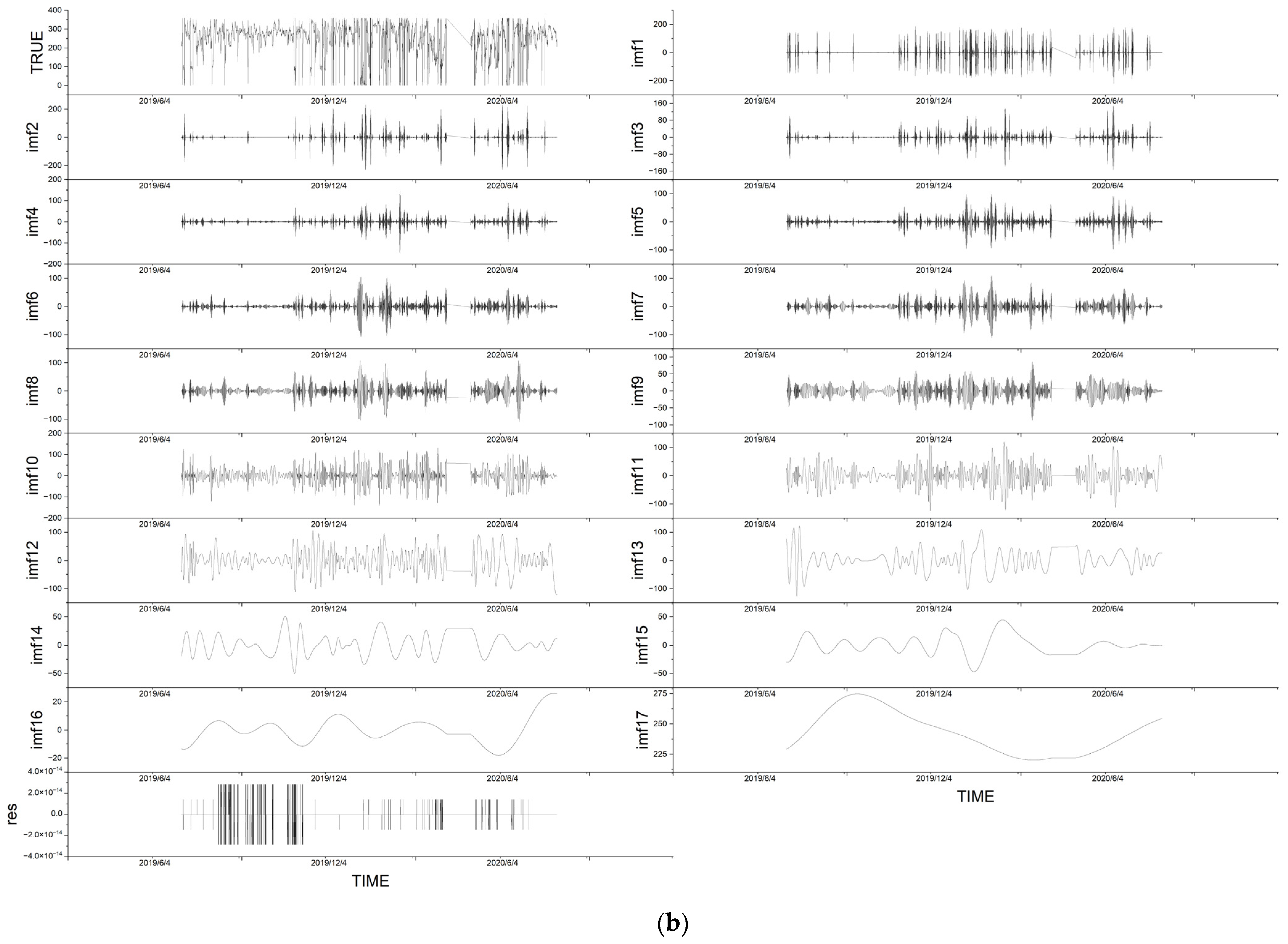
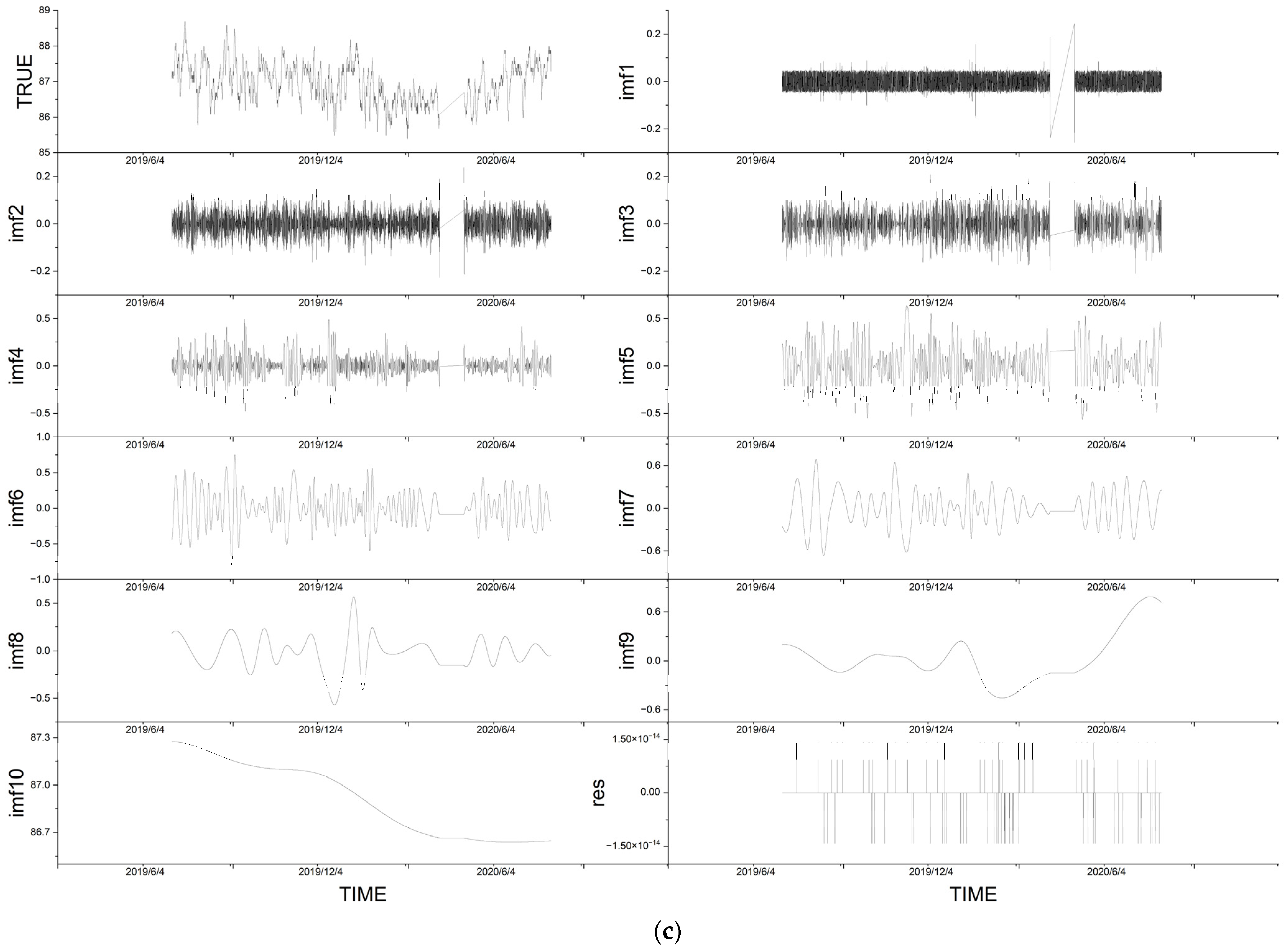
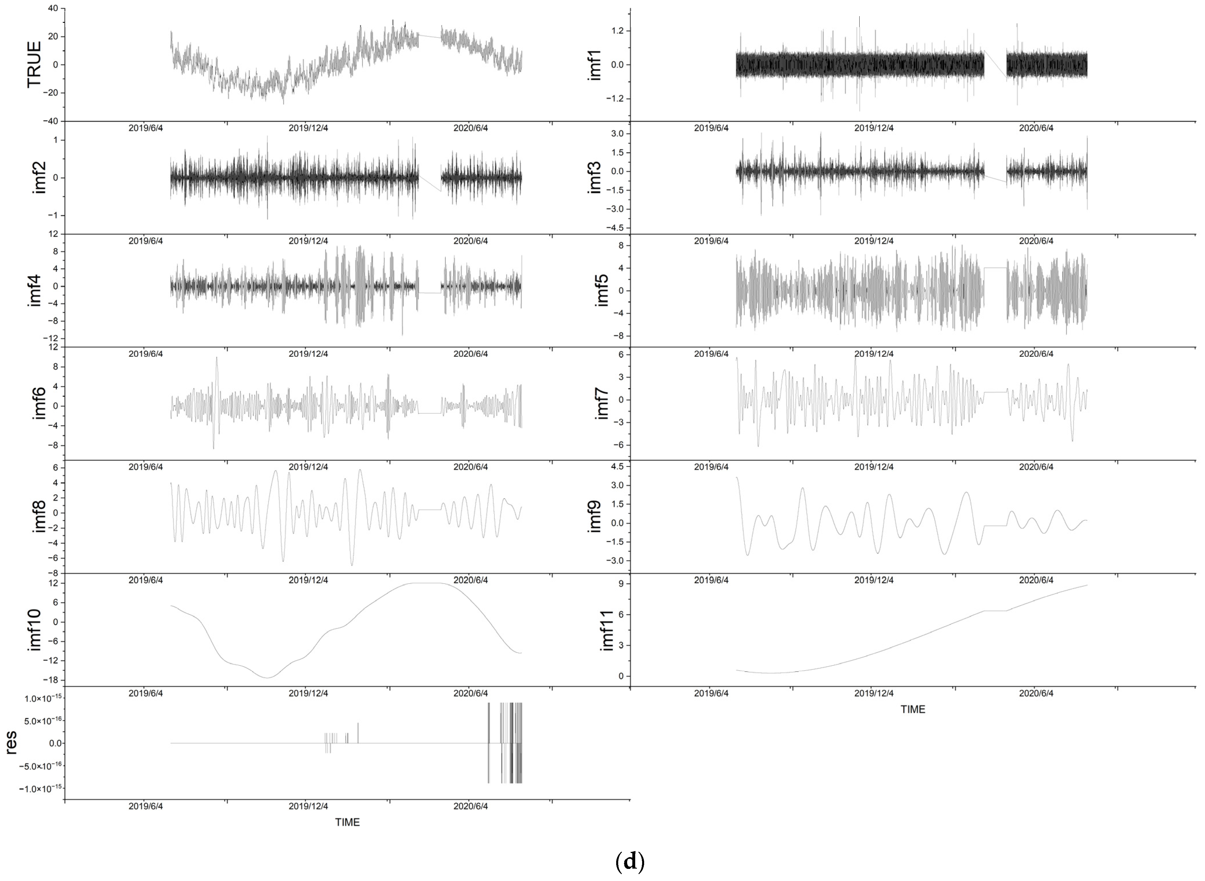
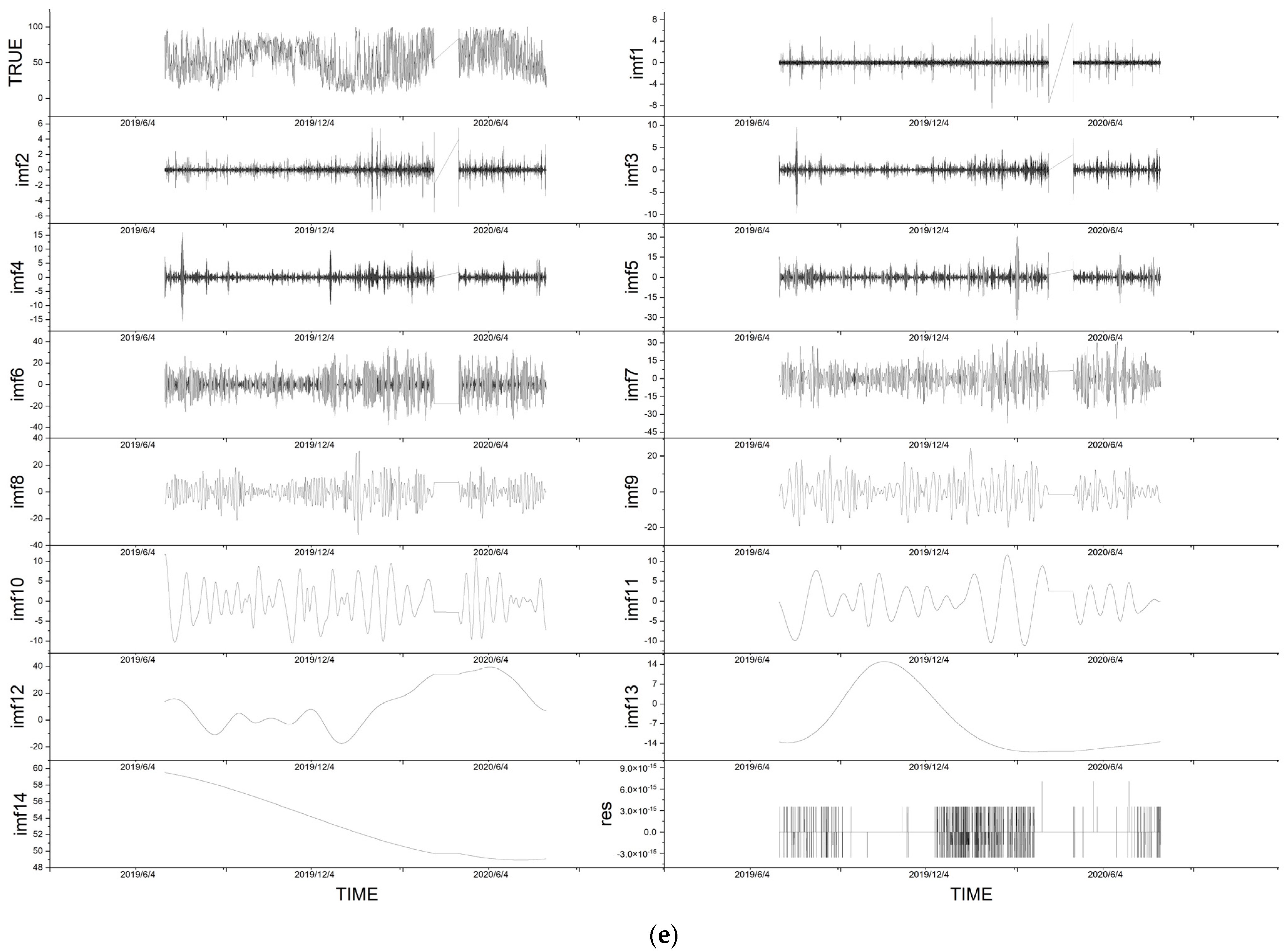
4.1. Decomposition by EMD
4.2. Dimensionality Reduction by PCA
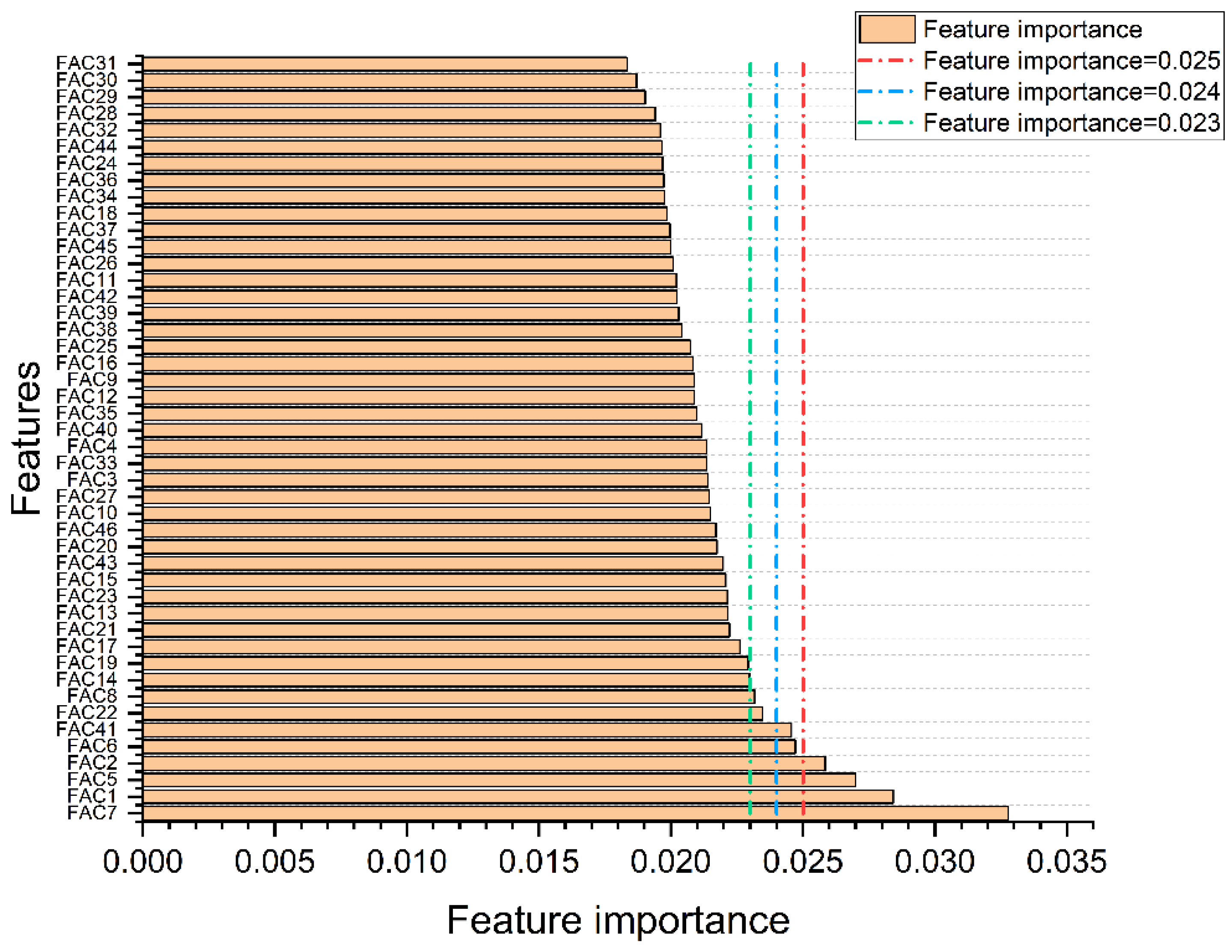
4.3. Feature Extraction by RF
4.4. Results and Comparison
4.4.1. Model Parameters
4.4.2. Determination of RF Threshold
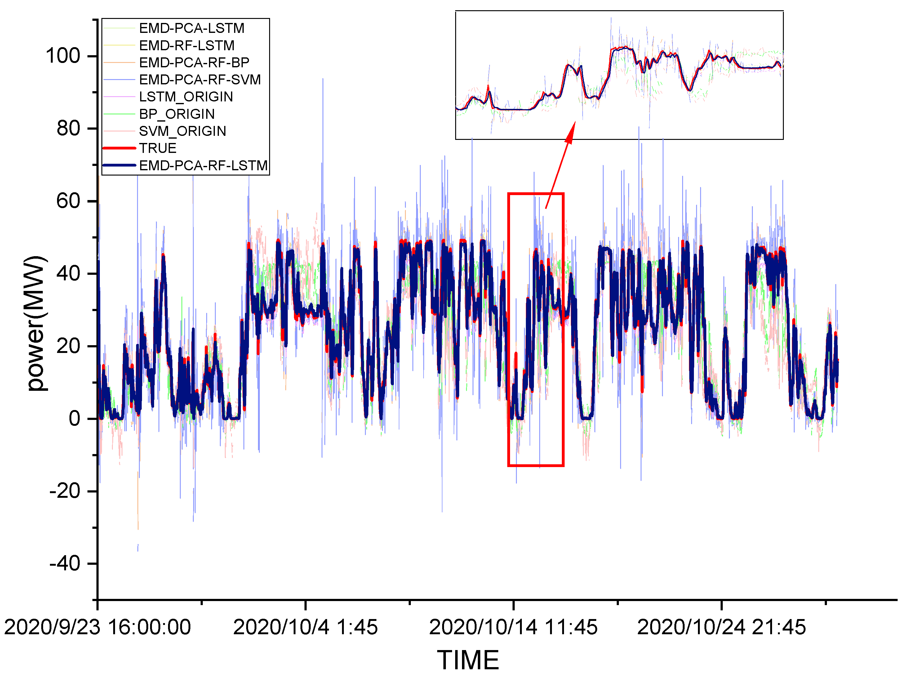
4.4.3. Analysis of Experimental Results
5. Conclusions
Author Contributions
Funding
Institutional Review Board Statement
Informed Consent Statement
Data Availability Statement
Conflicts of Interest
References
- Zheng, H.; Chen, H.P.; Li, H.; Zheng, Y.K. Wind Power Prediction Based on Wavelet Transform and RBF Neural Network. Lab. Res. Explor. 2019, 38, 36–39. [Google Scholar]
- Liu, C.; Lang, J. Wind Power Prediction Method Using Hybrid Kernel LSSVM with Batch Feature. Acta Autom. Sin. 2020, 46, 1264–1273. [Google Scholar]
- Gao, H.L.; Wei, X.; Ye, J.H.; Su, Y.P. Research on Wind Power Prediction Based on Optimal Combination of NSGA-II Algorithm. Water Power 2020, 46, 114–118. [Google Scholar]
- Wang, Y.; Zhang, N.; Kang, C.Q.; Miao, M.; Shi, R.; Xia, Q. An Efficient Approach to Power System Uncertainty Analysis with High-Dimensional Dependencies. IEEE Trans. Power Syst. 2018, 33, 2984–2994. [Google Scholar] [CrossRef]
- Yang, M.; Chen, X.X.; Du, J.; Cui, Y. Ultra-Short-Term Multistep Wind Power Prediction Based on Improved EMD and Reconstruction Method Using Run-Length Analysis. IEEE Access 2018, 6, 31908–31917. [Google Scholar] [CrossRef]
- Yang, M.; Huang, B.Y.; Jiang, B. Real-time Wind Power Prediction Based on Probability Distribution and Gray Relational Decision-making. Proc. CSEE 2017, 37, 7099–7108. [Google Scholar]
- Chen, H.; Zhang, J.Z.; Xu, C.; Tan, F.L. Short-term wind power forecast based on MOSTAR model. Power Syst. Prot. Control 2019, 47, 73–79. [Google Scholar]
- Cui, M.J.; Sun, Y.J.; Ke, D.P. Wind Power Ramp Events Forecasting Based on Atomic Sparse Decomposition and BP Neural Networks. Autom. Electr. Power Syst. 2014, 38, 6–11. [Google Scholar]
- Zendehboudi, A.; Baseer, M.A.; Saidur, R. Application of support vector machine models for forecasting solar and wind energy resources: A review. J. Clean. Prod. 2018, 199, 272–285. [Google Scholar] [CrossRef]
- Zhao, R.Z.; Ding, Y.F. Short-term prediction of wind power based on MEEMD-KELM. Electr. Meas. Instrum. 2020, 57, 92–98. [Google Scholar]
- Han, Z.F.; Jing, Q.M.; Zhang, Y.K.; Bai, R.Q.; Guo, K.M.; Zhang, Y. Review of wind power forecasting methods and new trends. Power Syst. Prot. Control 2019, 47, 178–187. [Google Scholar]
- Muzaffar, S.; Afshari, A. Short-Term Load Forecasts Using LSTM Networks. Energy Procedia 2019, 158, 2922–2927. [Google Scholar] [CrossRef]
- Kisvari, A.; Lin, Z.; Liu, X. Wind power forecasting—A data-driven method along with gated recurrent neural network. Renew. Energy 2021, 163, 1895–1909. [Google Scholar] [CrossRef]
- Memarzadeh, G.; Keynia, F. A new short-term wind speed forecasting method based on fine-tuned LSTM neural network and optimal input sets. Energy Convers. Manag. 2020, 213, 112824. [Google Scholar] [CrossRef]
- Chen, G.G.; Li, L.J.; Zhang, Z.Z.; Li, S.Y. Short-Term Wind Speed Forecasting with Principle-Subordinate Predictor Based on Conv-LSTM and Improved BPNN. IEEE Access 2020, 8, 67955–67973. [Google Scholar] [CrossRef]
- De Melo, G.A.; Sugimoto, D.N.; Tasinaffo, P.M.; Santos, A.H.; Cunha, A.M.; Dias, L.A. A New Approach to River Flow Forecasting: LSTM and GRU Multivariate Models. IEEE Lat. Am. Trans. 2019, 17, 1978–1986. [Google Scholar] [CrossRef]
- Li, J.Q.; Li, Q.J. Wind Power Prediction Method Based on Kriging and LSTM Network. Acta Autom. Sin. 2020, 41, 241–247. [Google Scholar]
- Wang, Y.N.; Xie, D.; Wang, X.T.; Li, G.J.; Zhu, M.; Zhang, Y. Prediction of Interaction Between Grid and Wind Farms Based on PCA-LSTM Model. Proc. CSEE 2019, 39, 4070–4081. [Google Scholar]
- Shi, J.R.; Zhao, D.M.; Wang, L.H.; Jiang, T.X. Short-term wind power prediction based on RR-VMD-LSTM. Power Syst. Prot. Control 2021, 49, 63–70. [Google Scholar]
- Zhang, Q.; Tang, Z.H.; Wang, G.; Yang, Y.; Tong, Y. Ultra-Short-Term Wind Power Prediction Model Based on Long and Short Term Memory Network. Acta Autom. Sin. 2021, 42, 275–281. [Google Scholar]
- Lin, J.; Ma, J.; Zhu, J.G.; Cui, Y. Short-Term Load Forecasting Based on LSTM Networks Considering Attention Mechanism. Int. J. Electr. Power Energy Syst. 2022, 137, 107818. [Google Scholar] [CrossRef]
- Zhu, K.D.; Li, Y.P.; Mao, W.B.; Li, F.; Yan, J.H. LSTM enhanced by dual-attention-based encoder-decoder for daily peak load forecasting. Electr. Power Syst. Res. 2022, 208, 107860. [Google Scholar] [CrossRef]
- Chung, W.H.; Gu, Y.H.; Yoo, S.J. District heater load forecasting based on machine learning and parallel CNN-LSTM attention. Energy 2022, 246, 123350. [Google Scholar] [CrossRef]
- Qu, J.Q.; Qian, Z.; Pei, Y. Day-ahead hourly photovoltaic power forecasting using attention-based CNN-LSTM neural network embedded with multiple relevant and target variables prediction pattern. Energy 2021, 232, 120996. [Google Scholar] [CrossRef]
- Hu, H.L.; Wang, L.; Tao, R. Wind speed forecasting based on variational mode decomposition and improved echo state network. Renew. Energy 2021, 164, 729–751. [Google Scholar] [CrossRef]
- Zhang, D.; Peng, X.G.; Pan, K.D.; Liu, Y. A novel wind speed forecasting based on hybrid decomposition and online sequential outlier robust extreme learning machine. Energy Convers. Manag. 2019, 180, 338–357. [Google Scholar] [CrossRef]
- Zhao, Q.; Huang, J.T. On ultra-short-term wind power prediction based on EMD-SA-SVR. Power Syst. Prot. Control 2020, 48, 89–96. [Google Scholar]
- Huang, B.Z.; Yang, J.H.; Shen, H.; Ye, J.G.; Huang, J.H. Power Optimization Control of District Drive Wave Power System Based on FFT. Acta Autom. Sin. 2021, 42, 206–213. [Google Scholar]
- Liang, S.J. Research on Time-domain Waveform Optimization of Digital Echo Signal Based on FFT. Fire Control Command Control 2021, 46, 73–77. [Google Scholar]
- Fang, B.W.; Liu, D.C.; Wang, B.; Yan, B.K.; Wang, X.T. Short-term wind speed forecasting based on WD-CFA-LSSVM model. Power Syst. Prot. Control 2016, 44, 37–43. [Google Scholar]
- Tian, Z.D.; Li, S.J.; Wang, Y.H.; Gao, X.W. Short-Term Wind Speed Combined Prediction for Wind Farms Based on Wavelet Transform. Transactions of China. Electrotech. Soc. 2015, 30, 112–120. [Google Scholar]
- Chen, Y.R.; Dong, Z.K.; Wang, Y.; Su, J.; Han, Z.L.; Zhou, D.; Zhang, K.; Zhao, Y.S.; Bao, Y. Short-term wind speed predicting framework based on EEMD-GA-LSTM method under large scaled wind history. Energy Convers. Manag. 2021, 227, 113559. [Google Scholar] [CrossRef]
- Fan, C.D.; Ding, C.K.; Zheng, J.H.; Xiao, L.Y.; Ai, Z.Y. Empirical Mode Decomposition based Multi-objective Deep Belief Network for short-term power load forecasting. Neurocomputing 2020, 388, 110–123. [Google Scholar] [CrossRef]
- Jiang, Z.Y.; Che, J.X.; Wang, L. Ultra-short-term wind speed forecasting based on EMD-VAR model and spatial correlation. Energy Convers. Manag. 2021, 250, 114919. [Google Scholar] [CrossRef]
- Sulaiman, S.M.; Jeyanthy, P.A.; Devaraj, D.; Shihabudheen, K.V. A novel hybrid short-term electricity forecasting technique for residential loads using Empirical Mode Decomposition and Extreme Learning Machines. Comput. Electr. Eng. 2022, 98, 107663. [Google Scholar] [CrossRef]
- Wang, X.; Huang, K.; Zheng, Y.H.; Li, L.X.; Lang, Y.B.; Wu, H. Short-term Forecasting Method of Photovoltaic Output Power Based on PNN/PCA/SS-SVR. Autom. Electr. Power Syst. 2016, 40, 156–162. [Google Scholar]
- Liu, J.; Wang, X.; Hao, X.D.; Chen, Y.F.; Ding, K.; Wang, N.B.; Niu, S.B. Photovoltaic Power Forecasting Based on Multidimensional Meteorological Data and PCA-BP Neural Network. Power Syst. Clean Energy 2017, 33, 122–129. [Google Scholar]
- Malvoni, M.; De Giorgi, M.G.; Congedo, P.M. Photovoltaic forecast based on hybrid PCA–LSSVM using dimensionality reducted data. Neurocomputing 2016, 211, 72–83. [Google Scholar] [CrossRef]
- Jian, Z.H.; Deng, P.J.; Zhu, Z.C. High-dimensional covariance forecasting based on principal component analysis of high-frequency data. Econ. Model. 2018, 75, 422–431. [Google Scholar] [CrossRef]
- Zhang, Y.G.; Chen, B.; Pan, G.F.; Zhao, Y. A novel hybrid model based on VMD-WT and PCA-BP-RBF neural network for short-term wind speed forecasting. Energy Convers. Manag. 2019, 195, 180–197. [Google Scholar] [CrossRef]
- Ziane, A.; Necaibia, A.; Sahouane, N.; Dabou, R.; Mostefaoui, M.; Bouraiou, A.; Khelifi, S.; Rouabhia, A.; Blal, M. Photovoltaic output power performance assessment and forecasting: Impact of meteorological variables. Sol. Energy 2021, 220, 745–757. [Google Scholar] [CrossRef]
- Zhang, S.Y.; Yang, K.; Xia, C.M.; Jin, C.L.; Wang, Y.Q.; Yan, H.X. Research on Feature Reduction and Classification of Pulse Signal Based on Random Forest. Mod. Tradit. Chin. Med. Mater. Mater. World Sci. Technol. 2020, 22, 2418–2426. [Google Scholar]
- Yu, W.M.; Zhang, T.T.; Shen, D.J. County-level spatial pattern and influencing factors evolution of carbon emission intensity in China: A random forest model. China Environ. Sci. 2022. [Google Scholar] [CrossRef]
- An, Q.; Wang, Z.B.; An, G.Q.; Li, Z.; Chen, H.; Li, Z.; Wang, Y.Q. Non-intrusive Load Identification Method Based on RF-GA-ELM. Sci. Technol. Eng. 2022, 22, 1929–1935. [Google Scholar]
- Lam, K.L.; Cheng, W.Y.; Su, Y.T.; Li, X.J.; Wu, X.Y.; Wong, K.H.; Kwan, H.S.; Cheung, P.C.K. Use of random forest analysis to quantify the importance of the structural characteristics of beta-glucans for prebiotic development. Food Hydrocoll. 2020, 108, 106001. [Google Scholar] [CrossRef]
- Chen, Y.Y.; Zheng, W.Z.; Li, W.B.; Huang, Y.M. Large group activity security risk assessment and risk early warning based on random forest algorithm. Pattern Recognit. Lett. 2021, 144, 1–5. [Google Scholar] [CrossRef]
- Makariou, D.; Barrieu, P.; Chen, Y.N. A random forest based approach for predicting spreads in the primary catastrophe bond market. Insur. Math. Econ. 2021, 101, 140–162. [Google Scholar] [CrossRef]
- Meng, Y.R.; Yang, M.X.; Liu, S.; Mou, Y.L.; Peng, C.H.; Zhou, X.L. Quantitative assessment of the importance of bio-physical drivers of land cover change based on a random forest method. Ecol. Inform. 2021, 61, 101204. [Google Scholar] [CrossRef]
- Li, D.; Jiang, F.X.; Chen, M.; Qian, T. Multi-step-ahead wind speed forecasting based on a hybrid decomposition method and temporal convolutional networks. Energy 2022, 238, 121981. [Google Scholar] [CrossRef]
- Zhang, Y.G.; Zhao, Y.; Kong, C.H.; Chen, B. A new prediction method based on VMD-PRBF-ARMA-E model considering wind speed characteristic. Energy Convers. Manag. 2020, 203, 112254. [Google Scholar] [CrossRef]
- Hu, S.; Xiang, Y.; Huo, D.; Jawad, S.; Liu, J.Y. An improved deep belief network based hybrid forecasting method for wind power. Energy 2021, 224, 120185. [Google Scholar] [CrossRef]
- Li, J.; Zhang, S.Q.; Yang, Z.N. A wind power forecasting method based on optimized decomposition prediction and error correction. Electr. Power Syst. Res. 2022, 208, 107886. [Google Scholar] [CrossRef]
- Tibshirani, R. Regression shrinkage and selection via the lasso. J. R. Stat. Soc. B 1996, 58, 267–288. [Google Scholar] [CrossRef]
- Chen, C.; Chen, D.L.; He, L.K. Short-term Forecast of Urban Natural Gas Load Based on BPNN-EMD-LSTM Combined Model. Saf. Environ. Eng. 2019, 26, 149–154. [Google Scholar]
- Huang, N.E.; Shen, Z.; Long, S.R.; Wu, M.C.; Shih, H.H.; Zheng, Q.; Yen, N.C.; Tung, C.C.; Liu, H.H. The empirical mode decomposition and the Hilbert spectrum for nonlinear and non-stationary time series analysis. Proc. R. Soc. A-Math. Phys. Eng. Sci. 1998, 45, 903–995. [Google Scholar] [CrossRef]
- Zhou, S.L.; Mao, M.Q.; Su, J.H. Prediction of Wind Power Based on Principal Component Analysis and Artificial Neural Network. Power Syst. Technol. 2011, 35, 128–132. [Google Scholar]
- Breiman, L. Random Forests. Mach. Learn. 2001, 45, 5–32. [Google Scholar] [CrossRef] [Green Version]
- Zhu, Q.M.; Li, H.Y.; Wang, Z.Q.; Chen, J.F.; Wang, B. Short-Term Wind Power Forecasting Based on LSTM. Power Syst. Technol. 2017, 41, 3797–3802. [Google Scholar]


| Data Field Name | Field Name Translation | Data Field Explanation |
|---|---|---|
| DATE | observation time point | From 0:00 on 1 October 2019 to 17:00 on 30 October 2020, observe every 15 min |
| humidity | humidity | Weather forecast humidity data (RH) |
| temp | temperature | Weather forecast temperature data (°C) |
| pressure | air pressure | Weather Forecast Air Pressure Data (KPa) |
| air_density | air density | Weather forecast air density data (kg/m3) |
| wind_dir | wind direction | Actual wind direction data from the wind measurement tower in the field (°) |
| wind_speed | wind speed | Actual wind speed data measured by wind measurement tower in the field (m/s) |
| power | wind power | Wind power output (MW) |
| Variable | Coefficient | Variable | Coefficient |
|---|---|---|---|
| wind_speed | 1.614955 | air_density | 0 |
| wind_dir | 0.097354 | humidity | −0.11514 |
| pressure | 0.006481 | temp | −0.12377 |
| Variable | IMFs | Residuals |
|---|---|---|
| wind_speed | 14 | 1 |
| wind_dir | 17 | 1 |
| pressure | 10 | 1 |
| temp | 11 | 1 |
| humidity | 14 | 1 |
| Component | Initial Eigenvalue | Component | Initial Eigenvalue | ||||
|---|---|---|---|---|---|---|---|
| Total | PV 1 | Accumulated % | Total | PV 1 | Accumulated % | ||
| 1 | 6.485 | 9.133 | 9.133 | 27 | 1.023 | 1.440 | 60.500 |
| 2 | 2.561 | 3.607 | 12.740 | 28 | 1.014 | 1.428 | 61.928 |
| 3 | 2.166 | 3.051 | 15.791 | 29 | 1.012 | 1.425 | 63.353 |
| 4 | 1.983 | 2.793 | 18.584 | 30 | 0.998 | 1.405 | 64.758 |
| 5 | 1.921 | 2.706 | 21.290 | 31 | 0.995 | 1.401 | 66.159 |
| 6 | 1.843 | 2.596 | 23.885 | 32 | 0.991 | 1.396 | 67.556 |
| 7 | 1.705 | 2.402 | 26.287 | 33 | 0.983 | 1.384 | 68.940 |
| 8 | 1.561 | 2.198 | 28.485 | 34 | 0.970 | 1.366 | 70.306 |
| 9 | 1.466 | 2.065 | 30.550 | 35 | 0.950 | 1.339 | 71.644 |
| 10 | 1.461 | 2.058 | 32.608 | 36 | 0.949 | 1.336 | 72.981 |
| 11 | 1.400 | 1.972 | 34.580 | 37 | 0.929 | 1.309 | 74.290 |
| 12 | 1.345 | 1.894 | 36.474 | 38 | 0.924 | 1.301 | 75.591 |
| 13 | 1.309 | 1.843 | 38.317 | 39 | 0.922 | 1.298 | 76.889 |
| 14 | 1.282 | 1.806 | 40.124 | 40 | 0.897 | 1.263 | 78.152 |
| 15 | 1.225 | 1.725 | 41.849 | 41 | 0.893 | 1.258 | 79.410 |
| 16 | 1.214 | 1.710 | 43.558 | 42 | 0.864 | 1.217 | 80.627 |
| 17 | 1.190 | 1.677 | 45.235 | 43 | 0.851 | 1.198 | 81.824 |
| 18 | 1.159 | 1.633 | 46.868 | 44 | 0.835 | 1.176 | 83.001 |
| 19 | 1.146 | 1.615 | 48.482 | 45 | 0.832 | 1.171 | 84.172 |
| 20 | 1.108 | 1.561 | 50.043 | 46 | 0.807 | 1.137 | 85.309 |
| 21 | 1.094 | 1.540 | 51.583 | 47 | 0.785 | 1.105 | 86.414 |
| 22 | 1.087 | 1.530 | 53.114 | 48 | 0.774 | 1.091 | 87.505 |
| 23 | 1.075 | 1.514 | 54.628 | … | … | … | … |
| 24 | 1.057 | 1.488 | 56.116 | 69 | 0.001 | 0.002 | 99.999 |
| 25 | 1.053 | 1.483 | 57.599 | 70 | 0.000 | 0.001 | 100.000 |
| 26 | 1.037 | 1.461 | 59.060 | 71 | 7.980 × 10⁻⁵ | 0.000 | 100.000 |
| Variable | Importance | Variable | Importance |
|---|---|---|---|
| FAC7 | 0.032787 | FAC17 | 0.022616 |
| FAC1 | 0.028421 | FAC21 | 0.022217 |
| FAC5 | 0.026995 | FAC13 | 0.022152 |
| FAC2 | 0.025839 | FAC23 | 0.022139 |
| FAC6 | 0.024718 | FAC15 | 0.022078 |
| FAC41 | 0.024562 | FAC43 | 0.021977 |
| FAC22 | 0.023467 | … | … |
| FAC8 | 0.023178 | FAC29 | 0.019019 |
| FAC14 | 0.022976 | FAC30 | 0.018696 |
| FAC19 | 0.022931 | FAC31 | 0.01834 |
| Parameter | Value of Parameter |
|---|---|
| train_size | 0.9 |
| epochs | 100 |
| batch_size | 48 |
| lr | 0.0001 |
| activation | relu |
| optimizer | adam |
| dense | 1/2/3 |
| train_size | 0.9 |
| epochs | 100 |
| batch_size | 48 |
| MSE | RMSE | MAE | R2 | |
|---|---|---|---|---|
| dense = 1 | 11.33006 | 3.36602 | 2.43616 | 0.953208 |
| dense = 2 | 7.30723 | 2.70319 | 1.70896 | 0.969822 |
| dense = 3 | 7.28741 | 2.69952 | 1.73744 | 0.969904 |
| MSE | RMSE | MAE | R2 | |
|---|---|---|---|---|
| dense = 1 | 8.64442 | 2.94014 | 2.15888 | 0.964299777 |
| dense = 2 | 7.35007 | 2.7111 | 1.72885 | 0.969645278 |
| dense = 3 | 7.69203 | 2.77345 | 1.83434 | 0.968233029 |
| MSE | RMSE | MAE | R2 | |
|---|---|---|---|---|
| dense = 1 | 8.4885 | 2.9135 | 2.0978 | 0.964943737 |
| dense = 2 | 7.64559 | 2.76507 | 1.8047 | 0.968424821 |
| dense = 3 | 7.26711 | 2.69576 | 1.73981 | 0.969987898 |
| MSE | RMSE | MAE | adj-R2 | The Percentage Enhancement of R2 | |
|---|---|---|---|---|---|
| SVM | 119.6383 | 10.93793 | 8.37387 | 0.5052151 | / |
| BP | 74.04614 | 8.60501 | 6.512 | 0.6937693 | / |
| LSTM | 12.42231 | 3.52453 | 2.6655 | 0.9486257 | / |
| EMD-PCA-RF-SVM | 68.24442 | 8.26102 | 5.02623 | 0.7175243 | 42.02% (Compared to SVM) |
| EMD-PCA-RF-BP | 35.44227 | 5.95334 | 3.73575 | 0.8532989 | 22.99% (Compared to BP) |
| EMD-RF-LSTM | 8.18422 | 2.86081 | 1.87817 | 0.9655112 | 1.77% (Compared to LSTM) |
| EMD-PCA-LSTM | 9.56465 | 3.09268 | 2.20952 | 0.9599812 | 1.19% (Compared to LSTM) |
| EMD-PCA-RF-LSTM | 7.26711 | 2.69576 | 1.73981 | 0.9699203 | 2.24% (Compared to LSTM) |
Publisher’s Note: MDPI stays neutral with regard to jurisdictional claims in published maps and institutional affiliations. |
© 2022 by the authors. Licensee MDPI, Basel, Switzerland. This article is an open access article distributed under the terms and conditions of the Creative Commons Attribution (CC BY) license (https://creativecommons.org/licenses/by/4.0/).
Share and Cite
Wang, D.; Cui, X.; Niu, D. Wind Power Forecasting Based on LSTM Improved by EMD-PCA-RF. Sustainability 2022, 14, 7307. https://doi.org/10.3390/su14127307
Wang D, Cui X, Niu D. Wind Power Forecasting Based on LSTM Improved by EMD-PCA-RF. Sustainability. 2022; 14(12):7307. https://doi.org/10.3390/su14127307
Chicago/Turabian StyleWang, Dongyu, Xiwen Cui, and Dongxiao Niu. 2022. "Wind Power Forecasting Based on LSTM Improved by EMD-PCA-RF" Sustainability 14, no. 12: 7307. https://doi.org/10.3390/su14127307
APA StyleWang, D., Cui, X., & Niu, D. (2022). Wind Power Forecasting Based on LSTM Improved by EMD-PCA-RF. Sustainability, 14(12), 7307. https://doi.org/10.3390/su14127307