Modelling Radiative and Convective Thermal Exchanges over a European City Center and Their Effects on Atmospheric Dispersion

Abstract

Micro-meteorological studies of urban flow and pollution dispersion often assume a neutral atmosphere and often the three-dimensional variation in temperature fields and flow around buildings is neglected in most building energy balance models. The aim of this work is to present the results of development and validation of a three-dimensional tool coupling thermal energy balance of the buildings and modelling of the atmospheric flow and dispersion in urban areas. To do so, a 3D microscale atmospheric radiative scheme has been developed in the atmospheric module of the computational fluid dynamics (CFD) code Code_Saturne adapted to detailed building geometries. The full coupling of the radiative transfer and fluid dynamics models has been validated with idealized cases. In this paper, our focus is to simulate and compare with measurements the diurnal evolution of the brightness surface temperatures and the momentum and energy fluxes for a neighborhood in the city center of Toulouse, in the southwest part of France. This is performed by taking into account the 3D effects of the flow around the buildings and all thermal exchanges, in real meteorological conditions, and compare them to aircraft infrared images and in situ measurements on a meteorological mast. The calculation mesh developed for the city center and the simulation conditions for the selected day of the field campaign are presented. The results are evaluated with the measurements from the Canopy and Aerosol Particles Interactions in TOulouse Urban Layer experiment (CAPITOUL). In addition, the second purpose of this work is to investigate a hypothetical release of passive pollutant dispersion in the same area of Toulouse under different thermal transfer conditions for the street and the buildings surfaces: neutral and 3D radiative transfer heating. The presence of heat transfer continually modifies the airflow field while the airflow in the neutral case reaches a stationary state. Compared to the neutral case, taking into account the thermal transfer enhances the turbulence kinetic energy and vertical velocity (especially at the roof level) due to buoyancy forces. The simulation results also show that the thermal effects considerably alter the plume shape.

1. Introduction

The influence of the urban thermal environment is currently receiving more attention than in the past, especially in the context of climate change. City residents are subjected to modified thermal environments, such as the urban heat island, as well as increased air pollution. In addition, a thermally comfortable environment is important for the inhabitants and commuters of urban areas. Current research concludes that anthropic emissions are the major sources of the pollution that causes urban air quality problems and greenhouse gases contributing to climate change [1]. In this context, sustainable development requires the anticipation through modelling of the interrelationship between buildings, their components, their surroundings (i.e., the surrounding atmosphere) and their occupants. In order to improve the urban microclimate, various countermeasures have been proposed and researched, such as roof greening, the use of high albedo paints (“white roofs”) and water-retentive materials. To optimize the choice of these adaptive options, detailed modelling including all the effects must be developed and validated.

In order to better understand the phenomena occurring at a neighborhood scale and to study different scenarios, more and more realistic simulation tools have been also developed, such as computational fluid dynamics (CFD) analysis. The behavior of the atmospheric urban canopy layer (UCL) is the result of the interactions between atmospheric structures induced by the urban heterogeneities. One important feature of the UCL is the urban surface energy balance (SEB). Recent research has sought to reconsider the problem of modelling the SEB, particularly to improve the modelling of thermo-radiative and aerodynamic phenomena. For instance, ref. [2] performed coupled simulations of convection, radiation and conduction to evaluate the outdoor thermal environment over different urban blocks, a high-rise area and a mid-rise area in the city of Tokyo in Japan, to compare the effects of measures such as the position of the heat release point of air-conditioning, greening, high surface albedo and traffic volume. The results showed that the effectiveness of moderation countermeasures differed according to the configuration of the urban blocks. Ref. [3] presented the SOLENE-microclimate model, including a soil model and an inner building thermal model, allowing them to compute the energy consumption of a building interacting with its urban environment. They are both integrated into the SOLENE (thermo-radiative simulation tool), which is then coupled to a CFD tool to calculate the air temperature, mass concentrations of moisture and the heat transfer coefficient. However, only the energy transport and moisture equations in the CFD tool are solved. Except for the initialization phase, the absence of the resolution of momentum equations does not allow one to take into account the natural and mixed convection movements of the airflow in the canopy. In order to learn more about the impacts of different proportions of green area, ref. [4] developed a classification scheme for typical European urban building types and have simulated them systematically with the microscale climate model ENVI-met. The simulation results were analyzed primarily in view of thermal advantages and disadvantages of increased green area and its effects on pollution dispersion and accumulation. It has been shown that especially in densely built-up block structures, greening with trees leads to higher pollution concentrations [5], while in more open structures the thermal advantages of greening, due to shadow effects, can be fully used to improve the microclimate. Ref. [6] investigated the impact of urban building morphology on local climate surface temperatures under wind conditions. The results showed that urban architectural patterns were one of the important drivers of urban climate change. Ref. [7] conducted field experiments with an open space under the influence of a sea breeze, pointing out that wind cooling performance is more significant in more ‘open’ areas. Ref. [8] then investigated the precinct ventilation performance and its influence on the urban heat island and outdoor thermal comfort within a compact high-rise gridiron precinct. The study confirmed that the combination of significant and different external meteorological conditions and precinct ventilation performance could not generate significant influence on the precinct ventilation performance.

The present research aims to accurately simulate the atmosphere and surfaces in urban environments at the microscale with an accurate representation of the geometry. Existing canopy models often use a statistical representation of buildings which is generally obtained through quantitative field surveys or qualitative estimates. However, in performing this geometric simplification, there is no way to ensure that the simplified geometry locally matches the actual city. In this work, we want to represent the energy and momentum exchanges in a portion of an existing city as realistically as possible. Thus, the objective is to fully model the three-dimensional (3D) airflow in the urban canopy in non-neutral conditions and therefore to take into account atmospheric radiation and heat transfer for complex geometries. A new 3D microscale radiative scheme has been previously implemented in the open-source CFD code Code_Saturne, described in detail by [9,10]. As a full thermo-radiative-convective coupling, the model was evaluated with idealized cases, using as a first step, a constant 3D wind field [9]. Ref. [11] then validated the full thermo-radiative-convective coupling by comparison with several surface wall temperatures from the Mock Urban Setting Test (MUST) field campaign [12,13,14]. Furthermore, in order to assess the thermal impact on the flow fields in different thermal conditions, ref. [15] extended the work of [11] to a lower wind speed and a higher building density than in MUST.

In order to validate this model as completely as possible with a large available experimental dataset in a real urban environment, we choose the Canopy and Aerosol Particles Interactions in TOulouse Urban Layer (CAPITOUL) experimental dataset [16]. Hereafter, we first give a brief overview of the experimental campaign. Following this, the mesh developed for the city center and the simulation conditions for the selected day of the campaign are presented. Afterwards, the simulation results are compared with the observations, including surface brightness temperatures, infrared images taken by an airborne infrared thermo-graph camera and in situ sensible heat flux, radiative flux and friction velocity measurements.

After this validation with a field campaign, a hypothetical city center passive release with and without the inclusion of the full thermal effect is studied. Removing the thermal effect amounts to using a neutral atmosphere which is often used in building wind-engineering neighborhood studies.

2. Model Description

The simulations are performed with the 3D open-source CFD code Code_Saturne, which can handle complex geometry and complex physics. The numerical solver employs a finite-volume approach for co-located variables on an unstructured mesh. Time discretization is achieved through a fractional step scheme, with a prediction-correction step [17].

Adapted for multi-scale atmospheric airflow (either neutral or stratified) and pollutant dispersion studies, the atmospheric module of Code_Saturne, described in [12] uses a detailed representation of the surfaces allowing a complex 3D spatial representation of wind speed, turbulence, and temperature. Two turbulent approaches are available in the module, the Reynolds-Averaged Navier–Stokes simulation (RANS) and Large Eddy Simulation (LES). The RANS approach with a k-ε turbulence closure was chosen for our simulations. We stress that despite the fact that the k-ε closure is generally unable to capture precisely the geometry-dependent large eddies in many complex flows and overestimates the dissipated energy, it gives a fairly acceptable accuracy with a reasonable computational time for this research work.

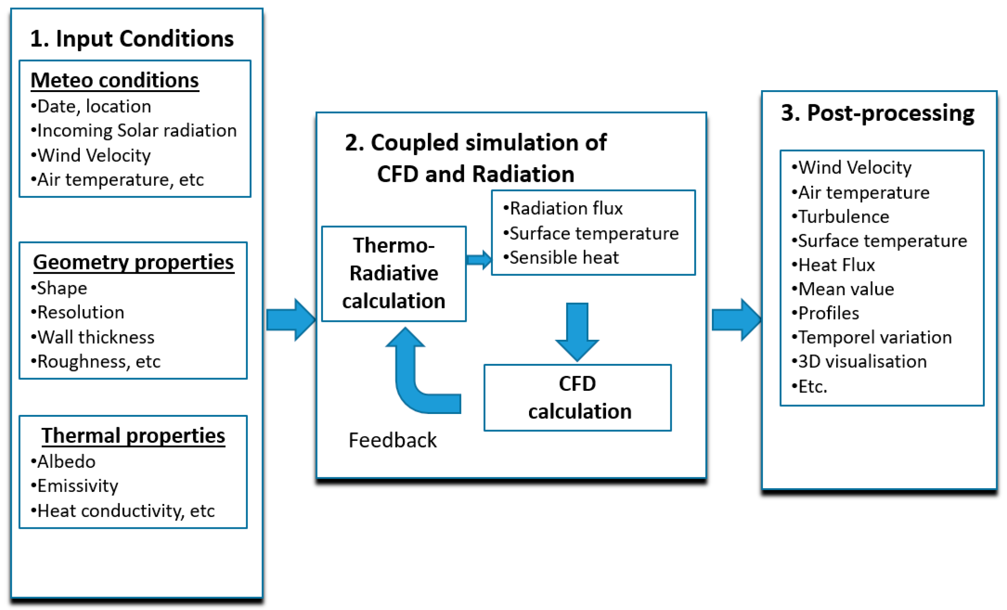
A framework describing the CFD modeling process is presented in Figure 1. In this study, the anthropogenic heat flux and the latent heat flux are neglected (but could be taken into account in the modeling with more experimental information). The advection fluxes are obtained by the resolution of the entire flow field. Thus, for each surface the surface energy balance (SEB) is expressed as:

$$Q_{cond}+Q_H=Q^{*},$$

(1)

where $Q_{cond}$ is the conductive heat flux ($\mathrm{W} {\mathrm{m}}^{-2}$) within the building or the ground subsurface, which links the surface temperature to the internal building or the deep soil temperature; $Q_H$ is the sensible heat flux ($\mathrm{W} {\mathrm{m}}^{-2}$), which depends on the local airflow intensity; and $Q^{*}$ is the net radiative flux ($\mathrm{W} {\mathrm{m}}^{-2}$).

3. Thermo-Radiative Model

The radiative fluxes are computed using the discrete ordinate method (DOM) [18] which solves the radiative transfer equation for gray non-diffusive semi-transparent media by the directional propagation of the radiation. In our models, the angular discretization has two resolutions: 32 or 128 directions, and the spatial discretization uses the same mesh as the CFD model. Taking into account both short- and long-wave radiation separately, a radiative heat transfer scheme available for combustion in Code_Saturne has been adapted. Described in detail by [9], the new atmospheric 3D radiative approach was developed in Code_Saturne for built-up areas. The main advantage of this model is that the radiative transfer equations are solved in the whole fluid domain and not only at solid faces (such as when using view factors), but also can be applied to non-transparent media (e.g., fog or pollution) as discussed in [19]. In this work, we consider a transparent atmosphere between the buildings at the microscale of our simulations.

4. Surface Temperature Model

As a key parameter, surface temperature T_sfc (K) is determined by the SEB and is fundamentally related to each of its component fluxes. In previous work [11], the surface temperature was obtained either with a force-restore approach or a wall thermal model. In order to take advantage of each model, in this work, we simulate the ground temperature with the force-restore method and the building surfaces (wall/roof) temperature with the wall thermal model. Hence, the simulated surface temperature is separately treated by the relationship:

4.1. Ground Temperature: Force-Restore Method

This simple approach is widely used for soil models in meteorological models [20].

$$\frac{\partial T_{sfc}}{\partial t}=\frac{\sqrt{2\omega }}{{\mu }_t}\left(L^{*}+S^{*}-Q_H\right)-\omega \left(T_{sfc}-T_{g/b}\right)$$

(2)

where $\omega$ ($\mathrm{Hz}$) is the Earth angular frequency; $L^{*}$ ($\mathrm{W} {\mathrm{m}}^{-2}$), $S^{*}$ ($\mathrm{W} {\mathrm{m}}^{-2}$), $Q_H$ ($\mathrm{W} {\mathrm{m}}^{-2}$) are, respectively, net long-wave, net short-wave and sensible heat flux; ${\mu }_t$ ($\mathrm{J} {\mathrm{m}}^{-2} {\mathrm{s}}^{-0.5} {\mathrm{K}}^{-1}$) is the thermal admittance and $T_{g/b}$ ($\mathrm{K}$) either deep soil or internal building temperature.

4.2. Building Surface Temperature: Wall Thermal Model

In the hypothesis of a single layer expressing the conduction term, it is described by:

$$\frac{\lambda }{e}\left(T_{sfc}-T_{int}\right)+h_f\left(T_{sfc}-T_a\right)=\epsilon \left(L_a+L_e-\sigma T_{sfc}^4\right)+\left(1-\alpha \right)\left(S_D+S_f+S_e\right),$$

(3)

where $\lambda$ ($\mathrm{W} {\mathrm{K}}^{-1} {\mathrm{m}}^{-1}$) is the average thermal conductivity of the wall, $e$ ($\mathrm{m}$) the thickness of the wall, $T_{int}$ ($\mathrm{K}$) the internal building temperature, $h_f$ ($\mathrm{W} {\mathrm{m}}^{-2} {\mathrm{K}}^{-1}$) the heat transfer coefficient and $T_a$ the external air temperature ($\mathrm{K}$).

In order to take into account the variation in the internal building temperature, it is computed with an incremental-adjustment method modified after [21] and similarly used by [22]:

$$T_{int}^{n+1}=T_{int}^{n-1}\left(\frac{\tau -\Delta t}{\tau }\right)+\overline{T}\left(\frac{\Delta t}{\tau }\right),$$

(4)

where $T_{int}^{n+1}$ ($\mathrm{K}$) and $T_{int}^{n-1}$ ($\mathrm{K}$) are the computed internal temperatures at the following and previous time step, respectively; $\Delta t$ is the time step ($\mathrm{s}$); $\tau$ ($\mathrm{s}$) refers to the number of seconds in a day and $\overline{T}$ ($\mathrm{K}$) is the average outside building surface temperatures computed at time step $n$ and set one by one. For a diurnal simulation, the initialized internal temperature value can be considered the same as the initialized outside surface temperature (e.g., $T_{sfc}$ at midnight) or the outside surface temperature at half hour intervals if the observation data are available.

4.3. Brightness Temperature

In this work, the simulated and measured brightness surface temperatures obtained from infrared imagery are compared. A brightness surface temperature ($T_{br}$ ($\mathrm{K}$)) is defined here as the temperature that yields an emitted broadband thermal radiance equivalent to the sum of the true broadband emitted radiance (with reduction due to gray body emissivity) and the broadband reflected radiance (after infinite reflections for canyon surfaces [22,23]:

$$T_{br}=\sqrt[4]{\epsilon T_{sfc}^4+\frac{\left(1-\epsilon \right)L^{\downarrow }}{\sigma }},$$

(5)

where $\epsilon$ is the long-wave emissivity, $\sigma$ the Stefan–Boltzmann constant and $L^{\downarrow }$ ($\mathrm{W} {\mathrm{m}}^{-2}$) incident long-wave radiation.

5. Convection Model

The surface convective heat flux must be computed to solve both the surface energy balance and determine the surface-air thermal gradient and therefore turbulent transport. In Code_Saturne, the convective heat transfer is computed in 3D for each surface patch. The buildings are explicitly defined in our simulations. Therefore, the detailed representation of the surface allows for a more complex 3D spatial representation of wind speed, turbulence and temperature than simple canopy averages or vertical profiles. A rough wall boundary condition, based on the logarithmic law modified by the stratification, is used. Usually, these modified laws are based on the Monin–Obukov similarity but are implicit and therefore need to be solved iteratively. Here an explicit approach based on the work of [24] and described in [25] is used.

The heat transfer coefficient $h_f$ is computed for each solid sub-facet, depending on the local friction velocity $u_{*}$ ($\mathrm{m} {\mathrm{s}}^{-1}$):

$$h_f=\frac{\rho C_p{u}_{*}\kappa f_h}{{\sigma }_{t}ln\left(\frac{d+z_0}{z_{0_T}}\right)\sqrt{f_m}},$$

(6)

where $C_p$ is specific heat ($\mathrm{J} \mathrm{k}{\mathrm{g}}^{-1} {\mathrm{K}}^{-1}$), $u_{*}$ is the friction velocity, $\kappa$ is the von Kármán constant, ${\sigma }_t$ the turbulent Prandtl number, $d$ ($\mathrm{m}$) is the distance of the cell center to the wall, $z_0$ the roughness length ($\mathrm{m}$), $z_{0_T}$ the thermal roughness length ($\mathrm{m}$) and $f_m$ and $f_h$ are the [24] stability functions which take a value of $1$ for neutral conditions. For vertical walls, the neutral conditions are applied.

6. Overview of CAPITOUL Field Experiment

The CAPITOUL campaign is a joint experiment, organized by the Centre National de Recherches Meteorologiques and other partners (Laboratoire d’Aérologie, Laboratoire des Mécanismes et Transferts en Géologie and ORAMIP local air quality agency), which took place in Toulouse in the southwest of France (4336′16.21″ N, 126′38.5″ E) from February 2004 to February 2005. It is an effort in urban climate, aiming to document the energetic exchanges between the surface and the atmosphere, the dynamics of the boundary layer over the city and the interactions between urban boundary layer and aerosol chemistry. A general view of the experiment, describing the goals, experimental set up and a summary of the results is given by [16].

6.1. Objectives and Description of the Site

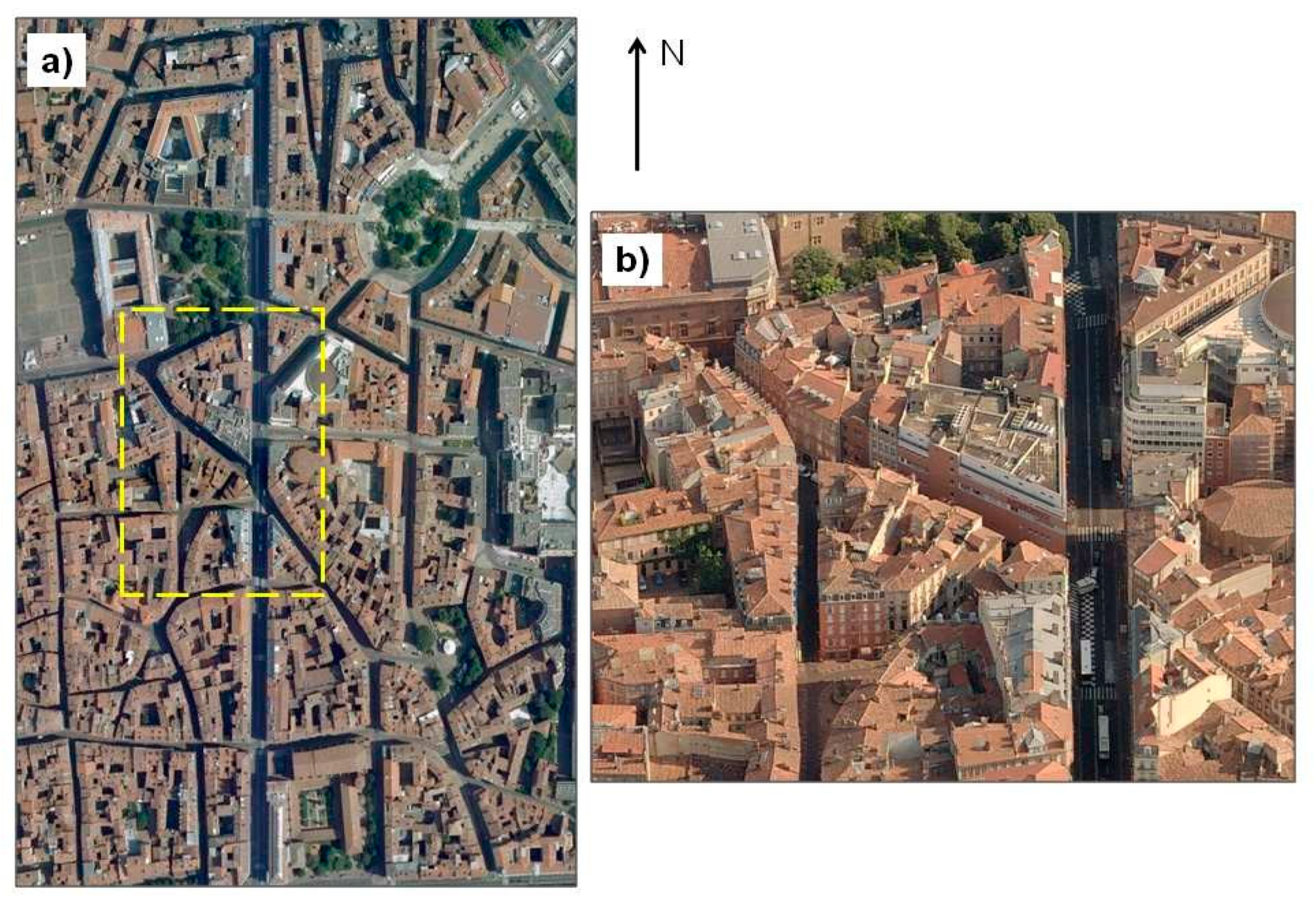
The old downtown, with an area of approximately 3.5 km², is generally made up of buildings four to five stories high with the walls primarily composed of brick and stone and the roofs of clay tile (Figure 1). The surrounding landscape is relatively flat with small rolling hills. Study of the energetic exchanges between the surface and the atmosphere was one of the objectives [26,27]. We briefly describe the data used in this study.

6.2. Geometric and Meteorological Data

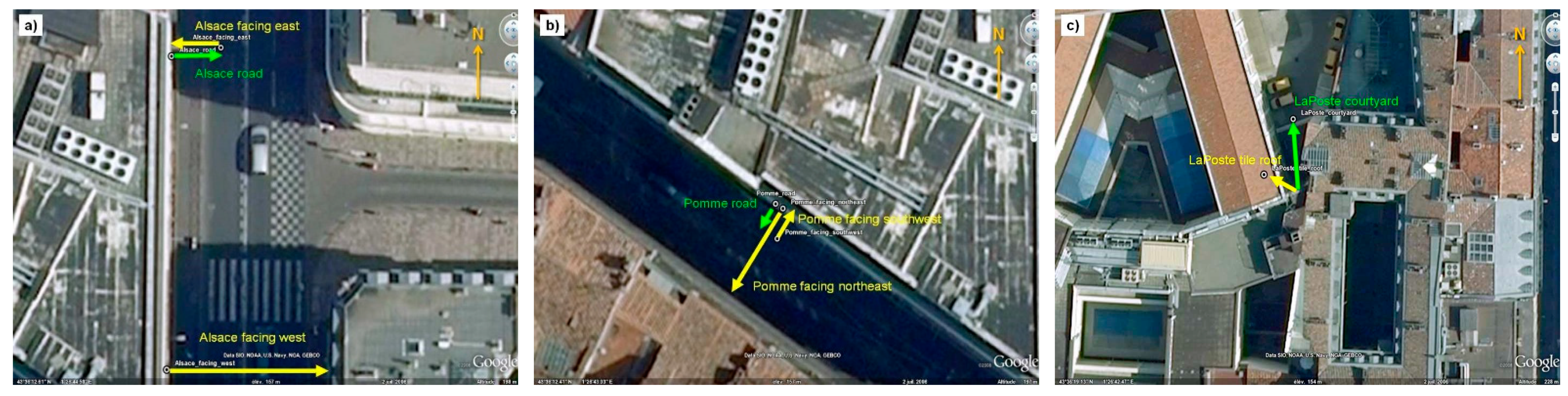
The study area is mainly located in the central site of Toulouse around the corner of two streets, Alsace-Lorraine and Pomme (yellow contour in Figure 2a,b). In this neighborhood, vegetation is very scarce, and buildings are around 20 m in height [27]. The base of the meteorological mast was on a roof at a height of 20 m, with the top of the mast being 47.5 m above the road (position shown by a star in Figure 3). It provided data, including short- and long-wave radiation flux, sensible heat, latent heat, air temperature, wind speed and direction, continuously from mid-February 2004 to early March 2005. All meteorological variables were sampled at one-second intervals and were recorded as one-minute averages [16].

6.3. Infrared Surface Temperature Measurements and Aircraft Data

A total of ten infrared thermometers were affixed to balconies or booms to record the surface temperatures of the roads, walls and roofs of the canyons. Described in detail in [26], four IRTs were positioned in the Alsace canyon to record surface temperatures of the two walls, the road and a roof. Three infrared thermometers were located in both the Pomme and Remusat canyons to observe the temperature of the two walls and the road in each canyon.

Infrared thermal (IRT) airborne images were also obtained during several intensive observation periods (IOP) of July 2004 with two airborne cameras on-board a Piper Aztec PA23 aircraft over the study area (flight 430: 0749–0816 UTC; flight 431: 1115–1150 UTC; flight 432: 1348–1423 UTC). The speed of the aircraft was 70 m s⁻¹ and the camera acquisition frequency was 4.3 frames per second. The flight height was about 460 m, which resulted in a resolution of between 1.5 and 3 m, depending on the sight angle [28,29].

7. Simulation Set-Up

Concerning urban canopy energetics issues, several papers on the CAPITOUL project have been published. Refs. [27,30] presents the modelling of the anthropogenic heat flux by the TEB urban scheme [31] and its validation against anthropogenic fluxes estimated by a new method using standard surface energy balance measurements. Based on the use of the SOLENE model coupled with a 3D model of the city providing information about the actual structure of the urban canopy, ref. [29] simulated the IRT anisotropy and the directional surface temperatures over the city of Toulouse. Ref. [32] imported the Toulouse urban database as a DART scene and tested the DART-TEB model for simulating remote sensing images and the radiation budget of urban canopies. Using SOLENE software, ref. [28] assessed the case of a small district of the city center for four independent sets of measurements for two complete diurnal cycles, in summer and in winter, by comparison with the thermo-radiative simulations.

Whereas earlier works estimated the sensible heat flux with simplified convection models, the heat transfer coefficient h_f is usually considered as a constant or a simple function of height. In order to model the microscale heat transfer with more accuracy by determining the surface-air thermal gradient that controls convective heat transfer and also examine the mechanisms (e.g., complex topographic influences on air motions), the CAPITOUL simulation with Code_Saturne was performed to investigate the thermo-dynamical impacts on the local atmosphere.

Choice of the Computational Domain and Mesh Strategy

The date of 15 July 2004 was selected from the CAPITOUL experiment. Considering Alsace-Lorraine and Pomme roads as the center of interest in the computational domain (Figure 2), the dimension of the 3D simulation domain is 891 × 963 × 200 m. The information about the 3D structure of the urban canopy was provided by the administrative authorities of Toulouse, who made the 3D database of the city available for the CAPITOUL project.

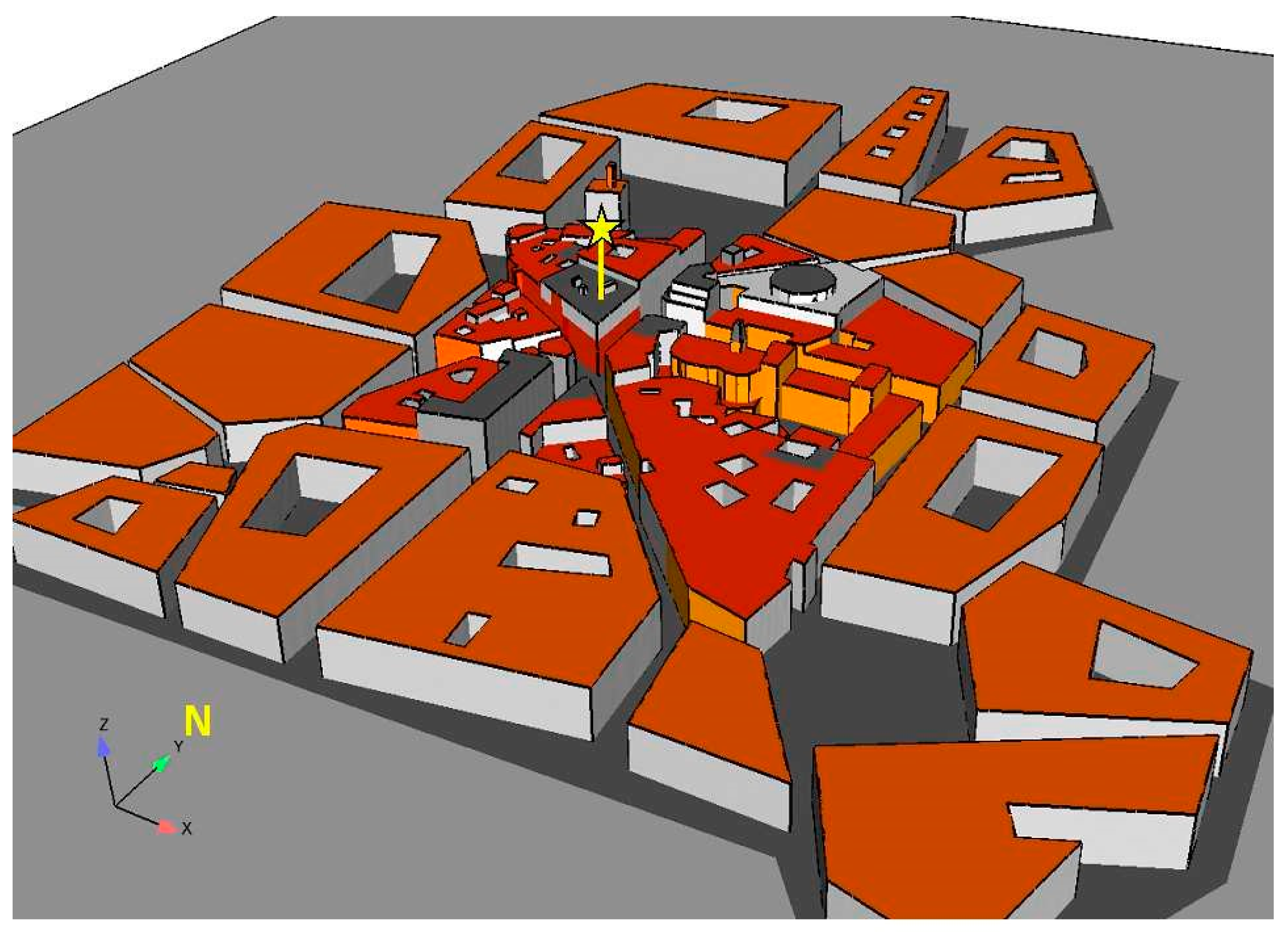
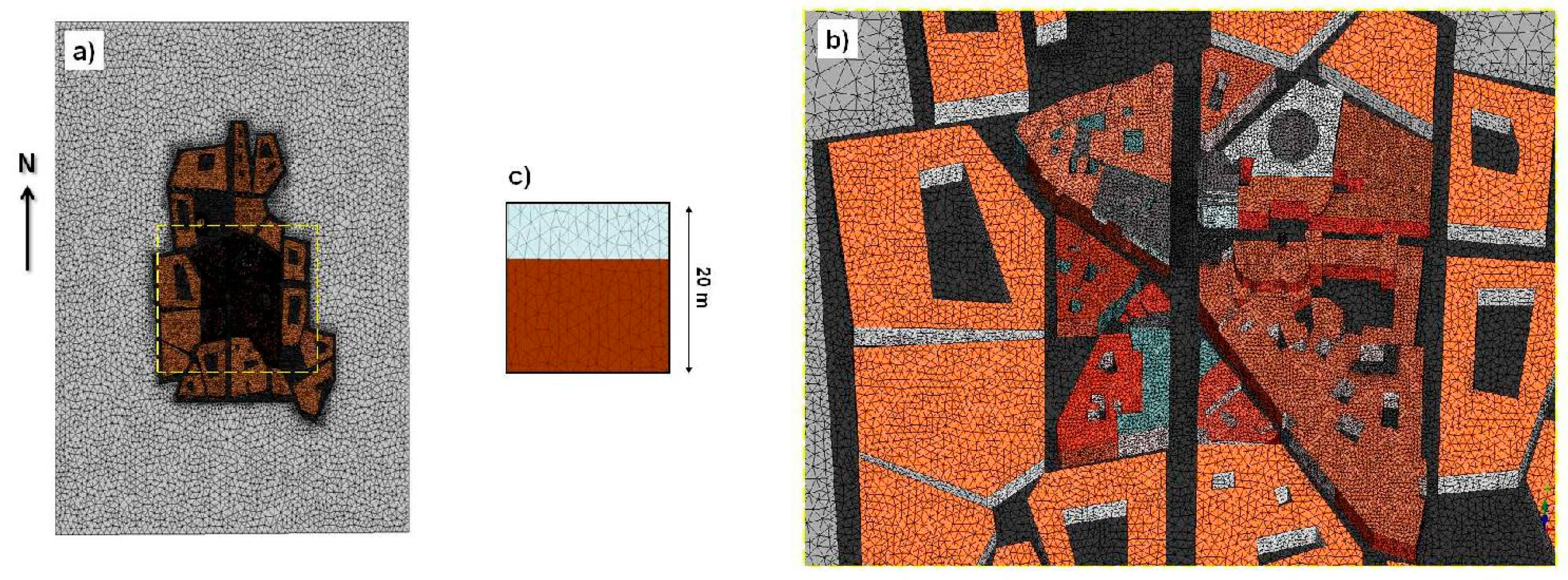
First, the urban database (AutoCAD format) of the Toulouse town hall is imported into the commercial mesher ICEM CFD. The urban elements in the database are not individual houses or buildings but a group of the walls and roofs, including a large number of internal fine walls which are unnecessary to be meshed. Moreover, the urban elements have a variety of heights but no soil element. Thus, before the meshing step, it was necessary to do preparatory work on the geometry. After a series of geometric optimizations (removing the internal surface, simplifying part of details, creating the ground then projecting the buildings onto it) a proper geometry topology was built, as shown in Figure 3. In a real urban environment, all obstacles cannot be resolved with sufficient detail, but their impact needs to be parametrized. We describe the strategy for this study as follows. From the boundary of the domain to the center, more geometric details were progressively retained. That is, the buildings at the Alsace-Lorraine and Pomme streets in the center study area were modeled with fine details. Following this, the surrounding buildings next to the center study area were simplified as urban blocks. Finally, the buildings in the region outside were treated with a high roughness value in this work. The volumetric mesh used here is an unstructured grid of about 4.5 million tetrahedral cells. The mesh resolution varies from 0.5 m near the center to 10 m far from the center zone (Figure 4).

The wind inlet boundary conditions are determined from measurements, using the meteorological mast which gives the wind velocity every 2 h (Figure 5a), wind direction (Figure 5b) and potential temperature profiles (Figure 5c).

From some pictures of Toulouse city, the roughness value was estimated depending on its location. Based on [27], the thermal properties such as surface conductivity and thickness are defined. The model parameters are summarized in

Table 1. Parameters applied in the CAPITOUL simulations.

Parameter	Unit	Value
Dynamic
Time-step	s	10
Zref	m	47.5
Uref	m s−1	3.21
φ	°	340
Roof z0	cm	10
Wall z0	cm	10
Street z0	cm	2
Radiative
Time-step	min	15
Roof z0T	cm	10
Wall z0T	cm	10
Street z0T	cm	2
αS		0.08
εR		0.9
εW		0.92
εS		0.95
λR	W K−1 m−1	0.83
λW	W K−1 m−1	1.15
eR	m	0.09
eW	m	0.3
µS	J m2 s−0.5 K−1	1330
Initial temperature values
Tair	°C	18.86
Alsace East (outside/inside)	°C	22.36/22.94
Alsace Road (outside/inside)	°C	23.18/25
Alsace West (outside/inside)	°C	21.32/22.23
Pomme SSWest (outside/inside)	°C	24.70/25.55
Pomme Route (outside/inside)	°C	23.33/25
Pomme NNEast (outside/inside)	°C	29.06/29.78
LaPoste Roof (outside/inside)	°C	11.13/10.36

. Since the values from [27] are averages over the 500-m radius around the surface energy balance station, inspecting some pictures of Toulouse from Google Maps, we further classified wall painting colors into four (rose, gray, whitewash and white) for the buildings in the center area, to estimate the albedo. Their values are given in

Table 2. Albedo classification of the building’s surfaces.

Paint Color	Albedo
White	0.6
Whitewash	0.5
Pink	0.3
Gray	0.15

.

8. Results and Discussion

8.1. Comparison of IRT Pictures

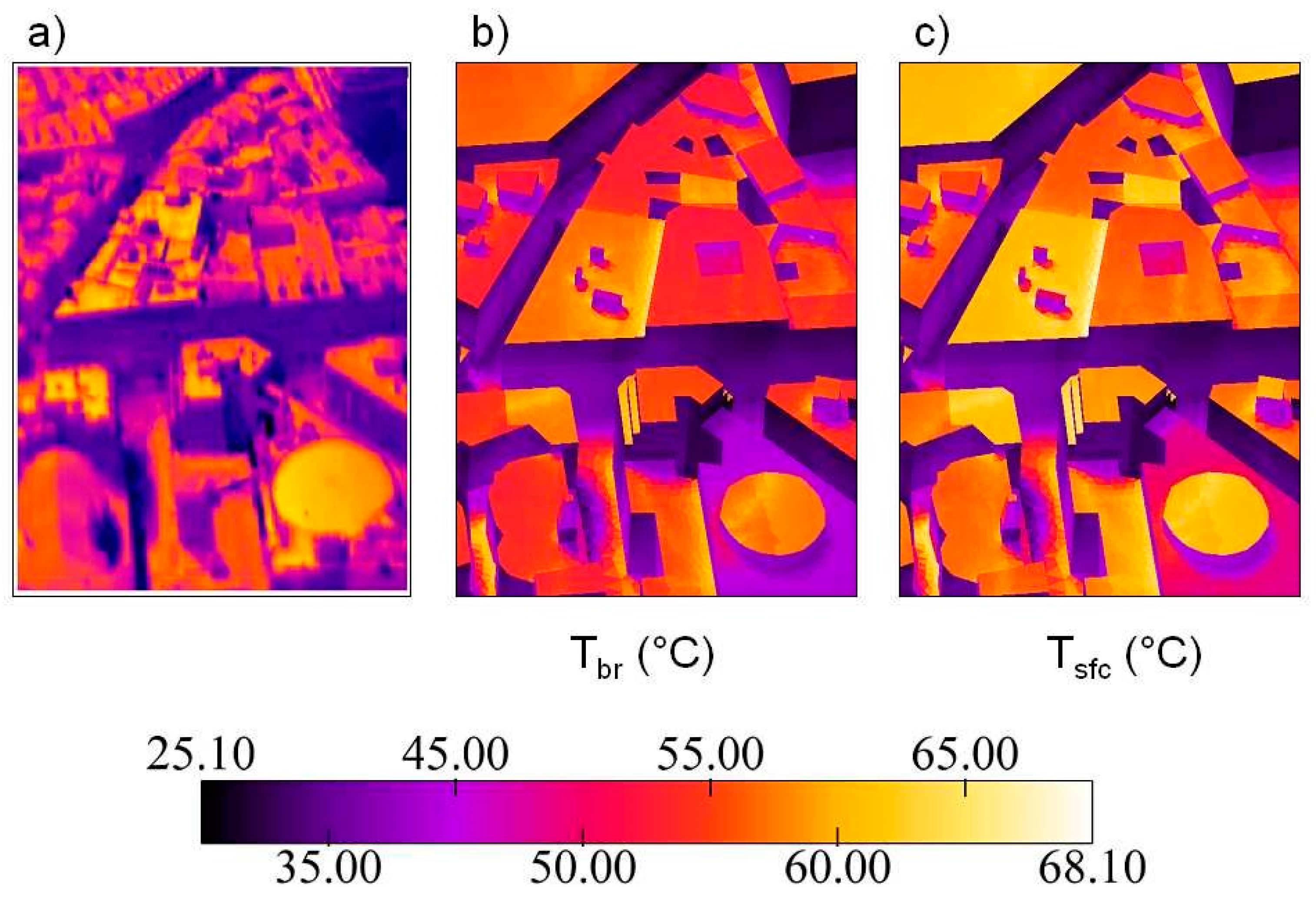
An infrared thermal (IRT) picture from the aircraft flight 432 of 15 July 2004 at 1412 UTC is shown in Figure 6a. In Figure 6b,c, we depict, respectively, the modeled brightness temperature and surface temperature with the radiative–convective full coupling active in the CFD. It should note that it is difficult to compare value by value because of the simplification of the geometry. However, since different albedos as a result of painting colors are distinguished, the model reproduced well the heterogeneity of the distribution of the brightness temperature, especially at roof level (Figure 6b). We can also note that if more details were kept, especially some slopes on central roof in our 3D model to create a more detailed distribution of the shadows on the roof, the simulated brightness roof temperature would be closer to the observations. The value of the modeled surface temperatures (Figure 6c) is obviously larger than the modeled brightness (e.g., about 3 °C difference on the roof), because one can see that the brightness temperature is approximately proportional to the product of the surface temperature and emissivity ($T_{br}\approx T_{sfc}{\epsilon }^{1/4}$, the emissivity being smaller than 1).

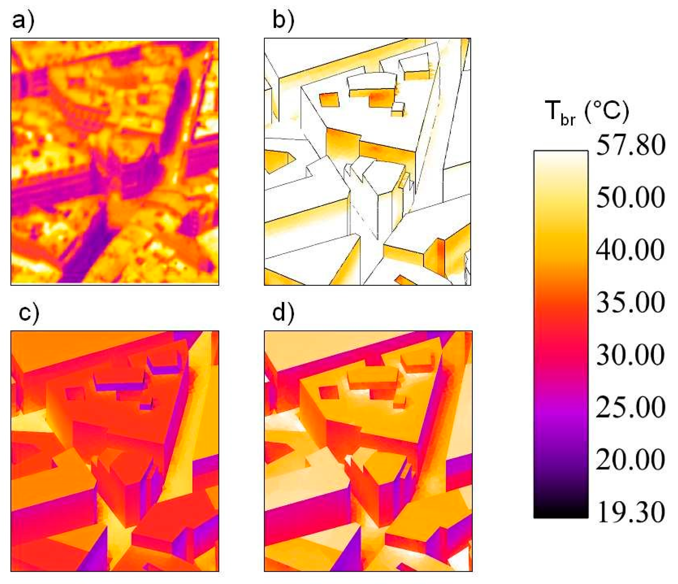
Figure 7 from (a) to (d) shows the measured and modeled brightness temperatures for the aircraft flight 431 at 1138 UTC, compared with three modelling approaches: radiative model only (Figure 7b), radiative and a constant heat transfer coefficient (Figure 7c) and radiative-convective full coupling (Figure 7d) using the hybrid thermal scheme for the streets and walls. The constant heat transfer coefficient (Figure 7c) was set in a manner similar to [23,28]. The result of the first simulation (Figure 7b, radiative scheme alone) shows that the brightness temperatures are obviously higher than the measurements. For clarity, an additional black contour is drawn to show the building structures. Especially on the roof, the difference is more than 25 °C. The modeled $T_{br}$ is out of color range.

Either taking a constant heat transfer coefficient, i.e., assuming a constant wind field in the domain or taking a variable heat transfer coefficient with full coupling, i.e., more realistically modelling the wind field, as expected, the results (Figure 7c,d) show a much better agreement with observation (Figure 7a) in comparison to radiative-model-only case (Figure 7b). From this IRT picture with this view (Figure 7a), in spite of the fact that all the elementary details were kept on the roofs with different orientations and slopes, the simulated temperatures represent well the spatial variability of the observed temperatures.

For the variable h_f case, the model-observation difference rarely exceeds 10 °C (Figure 7d). It should be noticed also, in the measurement (Figure 7a), that for the same roof and same orientation, the temperature may differ by more than 5 °C, for instance at the bottom right of the image. This may be due to heterogeneities in materials and geometry which cannot be all accounted for by modelling each individual area (or even every detail). For building walls, either shaded or sunlit, the difference between measurement and simulation is generally less than 5 °C. In the measurements, some horizontal faces (e.g., buildings at center left) are relatively warmer than others. This may be due to some external structures (e.g., balcony) that are not modeled but were exposed to the sun and therefore received more solar heating [23]. Regarding the streets, a minimum of three cells were set for the width; the model is able to simulate the sharpness of the shadow (Figure 7c,d). The portion of the street brightness temperatures near the buildings is well reproduced. The averaged difference is less than 3 °C and the simulated sunny portion is underestimated by about 5 °C.

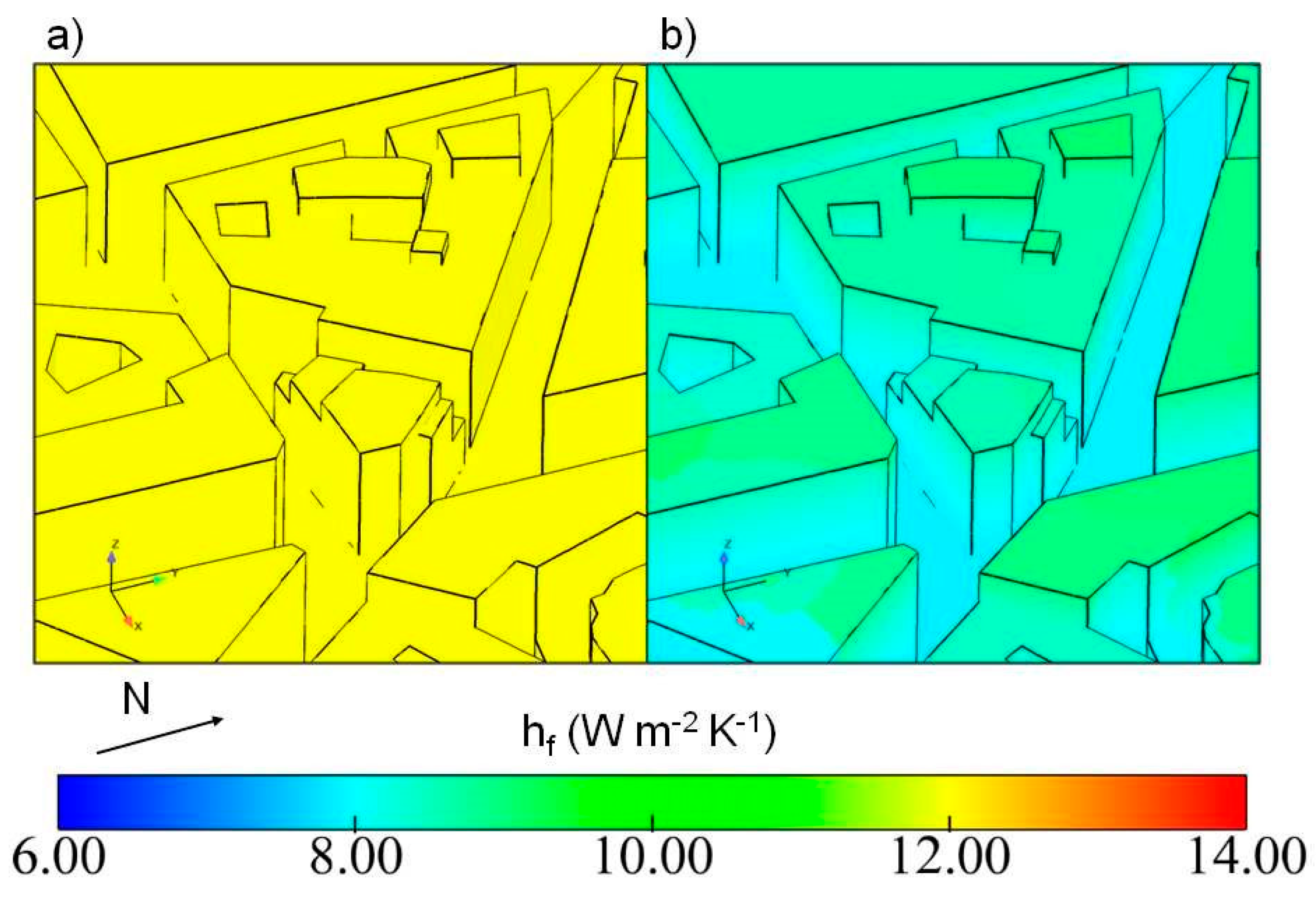
The difference between the constant h_f case and variable h_f case (Figure 7c,d) is also evident. These two different h_f are shown in Figure 8. With the constant h_f case, we see an overcooling of about 15 °C at roof level, 4 to 5 °C at the walls, 4 °C in shaded streets and 7 °C in sunlit streets (Figure 7c). The difference is due to the overestimation of the constant chosen value (h_f = 12) at this moment. In fact, the contribution of the variable h_f may be more important for the surface and air temperature when modelling the temporal evolution. For this reason, the simulation with full coupling for a diurnal evolution is performed in the next section.

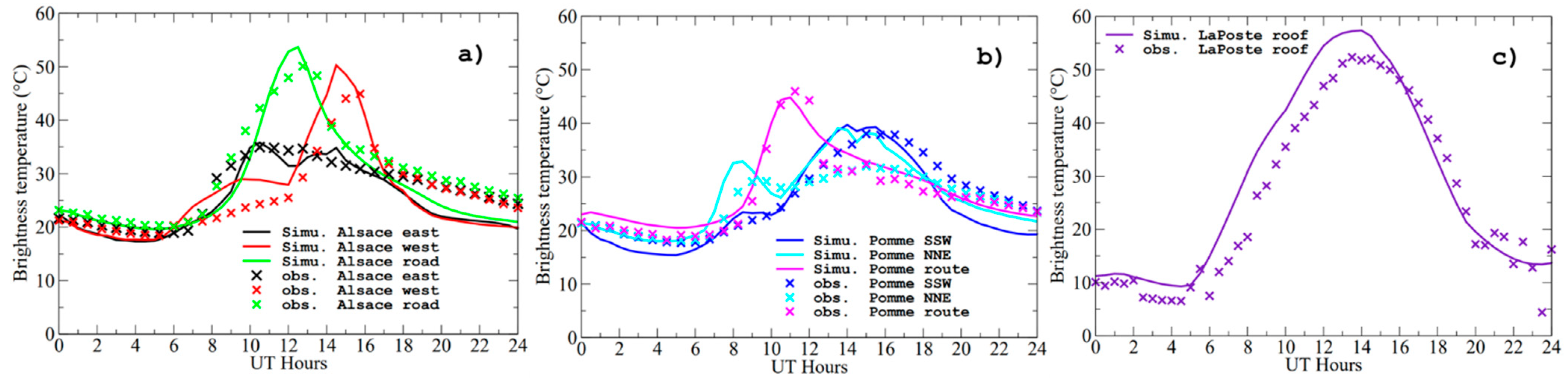
8.2. Comparison of the Local Diurnal Evolution of Brightness Surface Temperature $T_{br}$

Figure 9a–c present the model-observation comparison for the brightness surface temperatures of the diurnal cycle of 15 July 2004. The simulation is performed with full radiative-dynamic coupling. Hereafter, unless specified otherwise, all the results refer to full coupling simulations. The infrared radiometers provided the measured brightness temperatures. Their fixed positions around the central building of the study district are shown in Figure 10. Overall, the diurnal evolutions of the brightness surface temperatures at the local positions in the scene are correctly simulated.

For the faces of the Alsace street (black and red lines in Figure 9a), an overcooling of about 5 °C appears during the evening (1800 to 2400 UTC). However, for the Alsace west face, the model predicts a higher brightness temperature (red line in Figure 9a) from 0600 to 1200 UTC. Using the SOLENE model, [28] also reported a similar difference in surface temperature. They explained that this may be due to a sensor underestimation. The ground temperature was computed by the force-restore method which is well adapted for the soil model. The bias on the Alsace road (green line in Figure 9a) can be explained by the approximation of the modeled shadow. Indeed, values taken from the selected cell might be quite different from its neighborhood values.

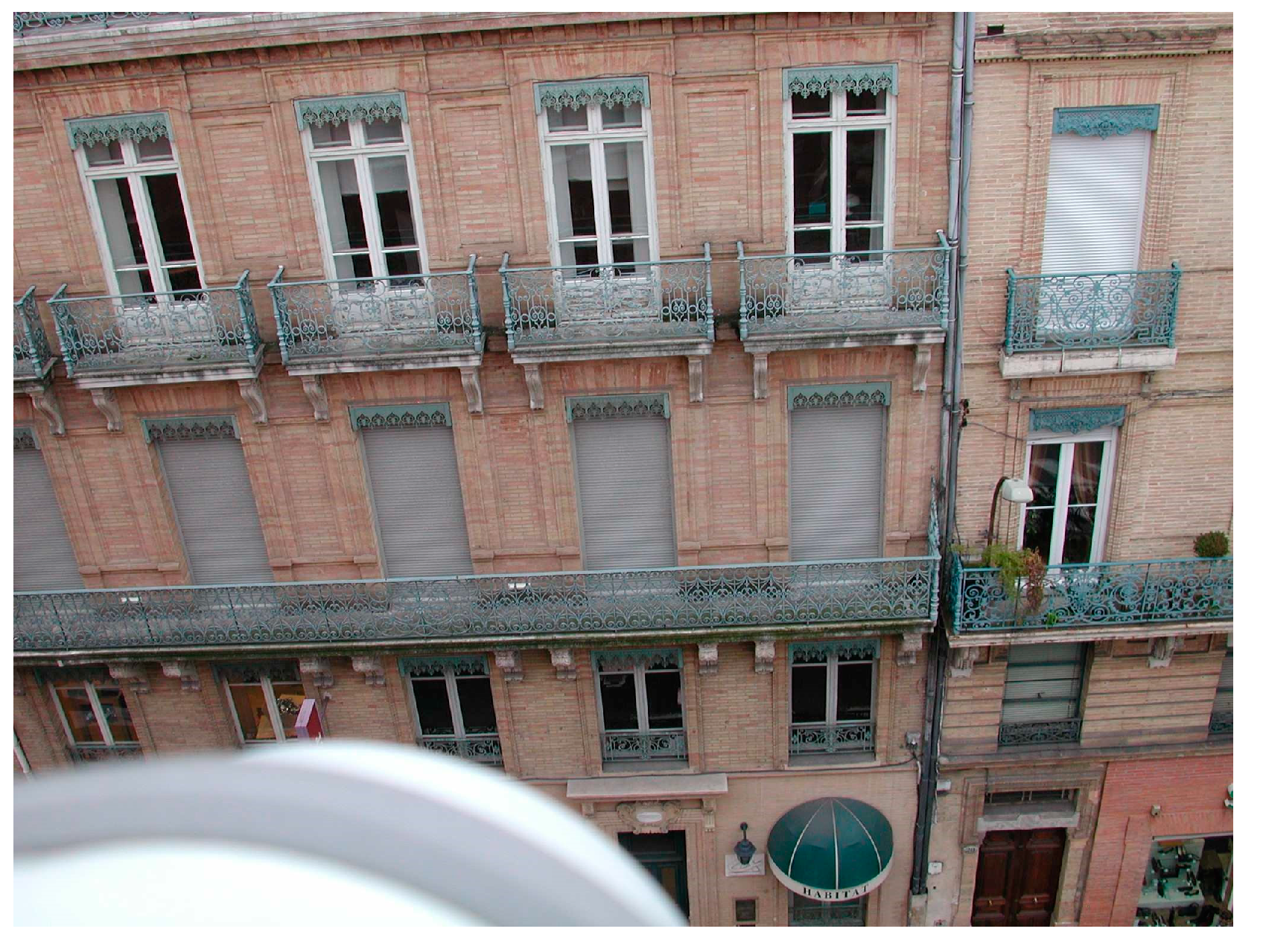
The brightness temperature of the Pomme route is best predicted (magenta line in Figure 9b). The primary model-observation disagreement occurs on Pomme northeast face (cyan line in Figure 9b) during the afternoon. The bias reaches 8 °C. One can adopt the same explanation as for the Alsace road. Moreover, from some photos (Figure 11), it can be found that there are numerous windows with white blinds on this side of the wall. The infrared radiometer might have detected a position where the white blinds were closed and therefore a higher temperature was measured. Another possibility is that windows were opened, and the ventilation in the canopy led to a lower internal building temperature which decreased the external temperature. Finding an explanation is a difficult task. First, there is an uncertainty in the observation. Second, there is a need to model this wall in more detail, maybe including the balcony and windows.

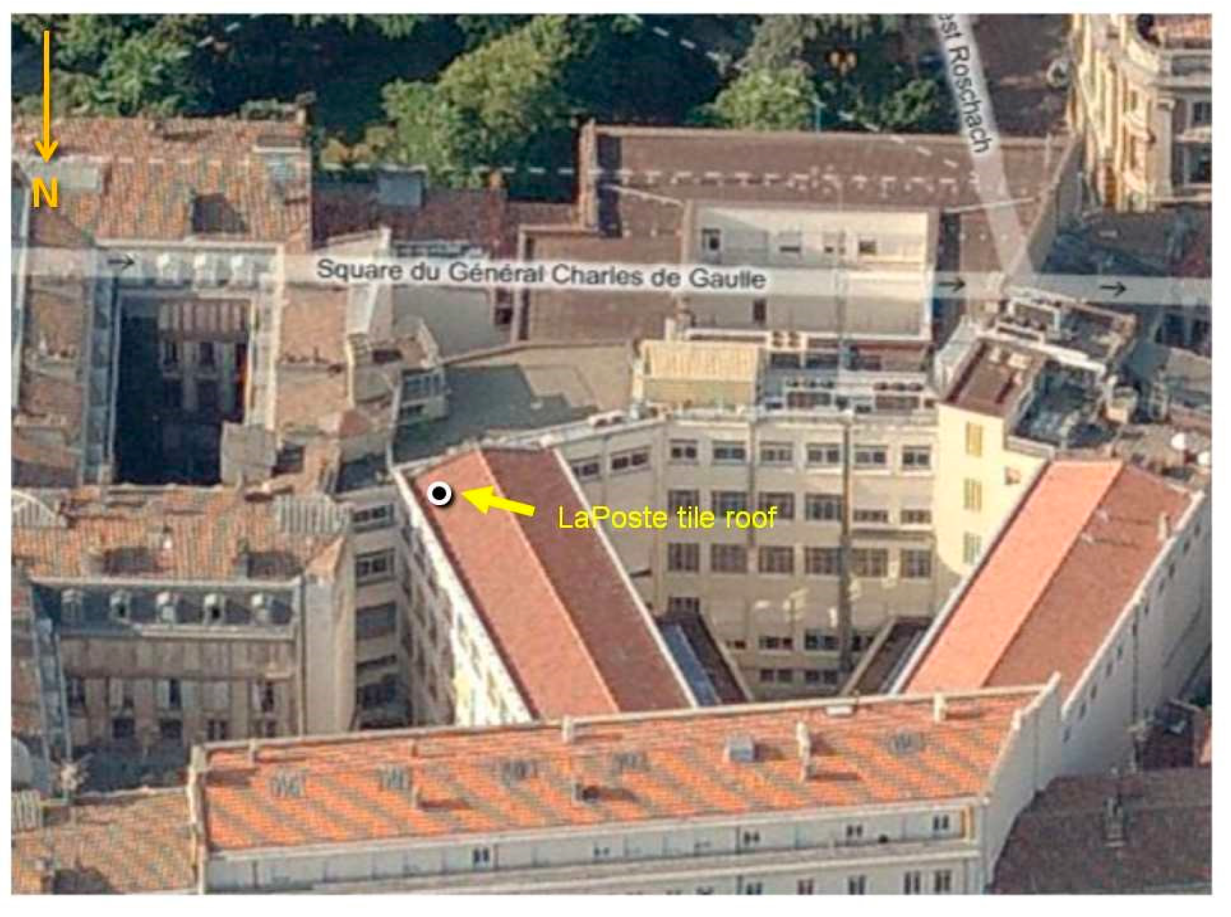
The modeled roof brightness temperature displays a good agreement with observation before sunrise and from late afternoon to midnight (Figure 9c). However, the model exhibits a significant advance in warming when the roof starts being sunlit. Actually, the sensor detecting roof brightness temperature was fixed on a building’s roof north of the mast (Figure 10c and Figure 12). This building was treated as a simple block in the 3D model (Figure 3). However, from Figure 10c and Figure 12, the complex structure of the roof can be observed. In particular, there are some small obstacles which are higher than the measured roof to the east but are not represented in the simulated scene. During the sunrise, the roof might be shaded due to these non-modeled detail structures. From the late afternoon, the sun shifts to another side. In that case no more small obstacles are higher than the measured roof and the bias disappears.

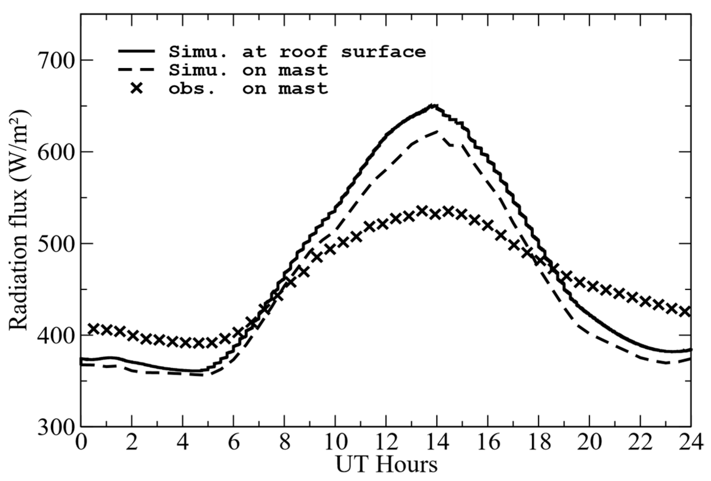
8.3. Outgoing Long-Wave Radiative Flux $L^{\uparrow }$

Figure 13 shows the model-observation comparison of long-wave radiation flux. The difference between the modeled outgoing long-wave radiation flux at the roof surface (full line) and on the mast (dashed line) is generally less than 20 W m⁻². However, both of them give an underestimation of about 20 W m⁻² during the night and a maximum overestimation of about 100 W m⁻² in daytime. In fact, these differences are related to the error on the roof temperature, i.e., underestimation in the night and overestimation in the day. We recall here that the outgoing infrared radiation flux depends strongly on the surface temperature because of the term $\epsilon \sigma T_{sfc}^4$.

To complete the discussion, we have the advantage, with the model, of being able to visualize the radiative flux inside the computational domain. Figure 14 illustrates the distribution of the outgoing infrared flux at 1030 UTC on the vertical center-plane and on the building surfaces. Significant variability can be observed on the center-plane. Relatively high values are found at the horizontal solid–air interface due to the fact that horizontal surfaces are warmer than vertical surfaces in the daytime.

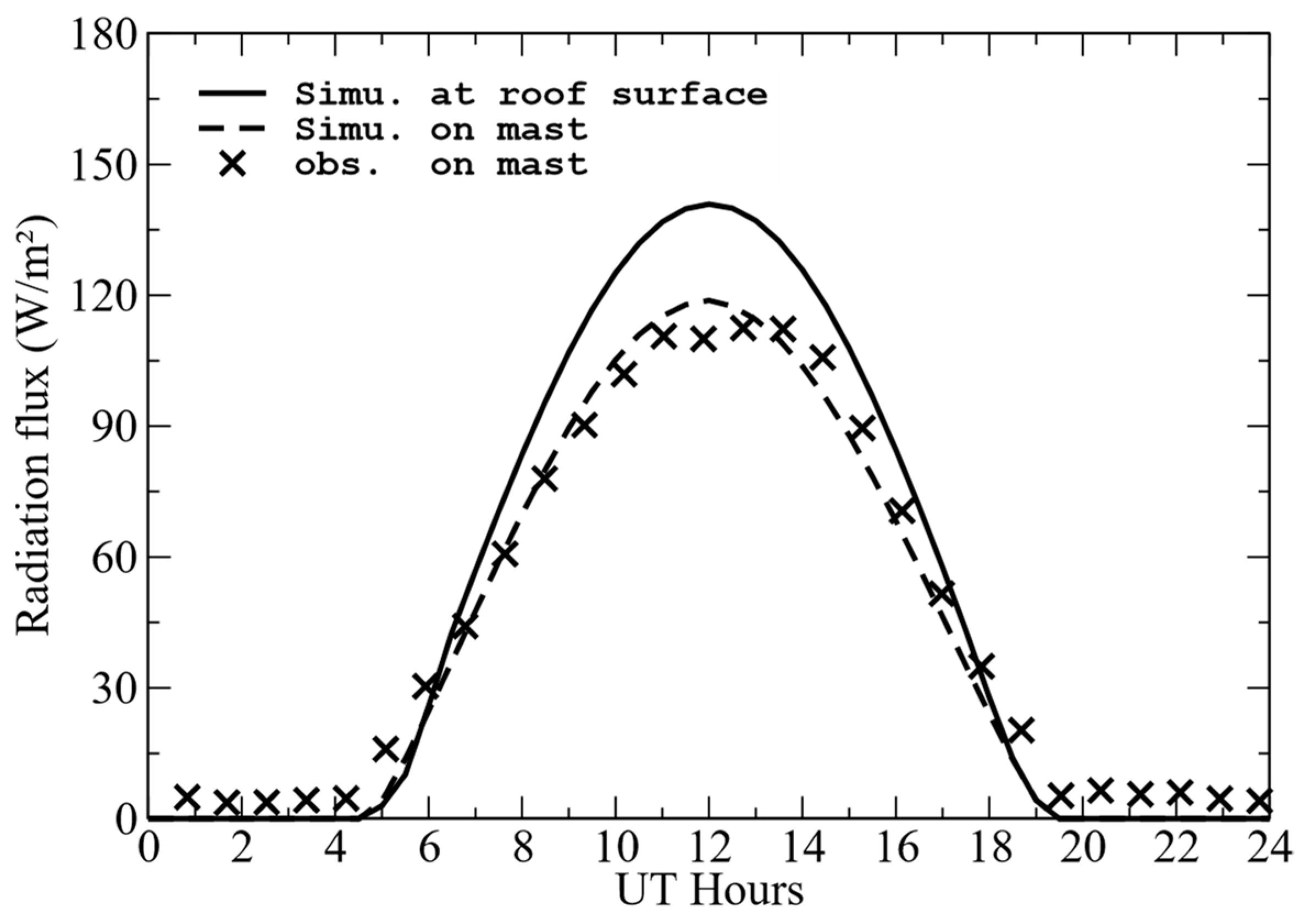
8.4. Outgoing Global Radiative Flux $S^{\uparrow }$

Figure 15 compares the modeled upward global solar flux with the measured one. The non-zero measured nighttime solar flux may be due to the sensor errors or the artificial lights from shopwindows, cars and streetlamps [28]. The upward solar flux can be estimated by

$$S^{\uparrow }=\alpha \left(S_D+S_f+S_e\right)$$

(7)

where $S_D$ ($\mathrm{W} {\mathrm{m}}^{-2}$) is the direct solar flux, $S_f$ ($\mathrm{W} {\mathrm{m}}^{-2}$) the solar flux diffused by the atmosphere above and $S_e$ ($\mathrm{W} {\mathrm{m}}^{-2}$) the flux diffused by the environment (i.e., from multi-reflection on the surfaces).

For this gray roof (Figure 10b), an albedo of 0.15 was set (Table 2). The same value was also proposed by [27] and was used in [28]. Compared to the observation, in spite of about 20 W m⁻² higher values at noon estimated by the model (full line), the agreement between measurement and model for the outgoing solar flux on the mast (dashed line) is very satisfactory.

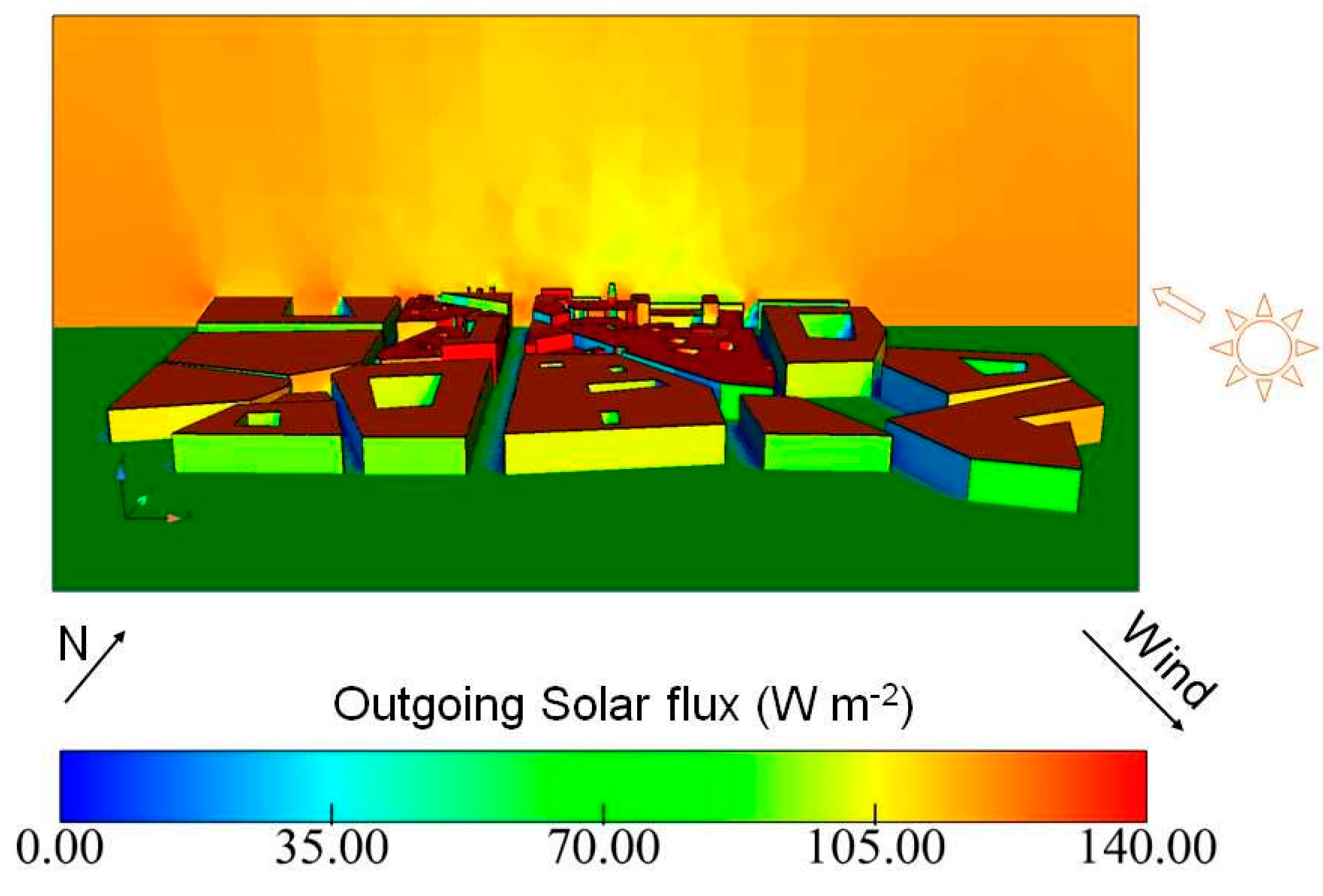
In the same manner as for the long-wave radiative flux, in Figure 16 the distribution of the outgoing global solar flux at 1030 UTC on the center-plane and on the surfaces is displayed. Through the visualization of the propagation of the radiative flux in the fluid domain, one can better understand the distribution of the shadow projected by the different structures. One can also readily identify surfaces with higher albedo since they reflect more solar radiation flux.

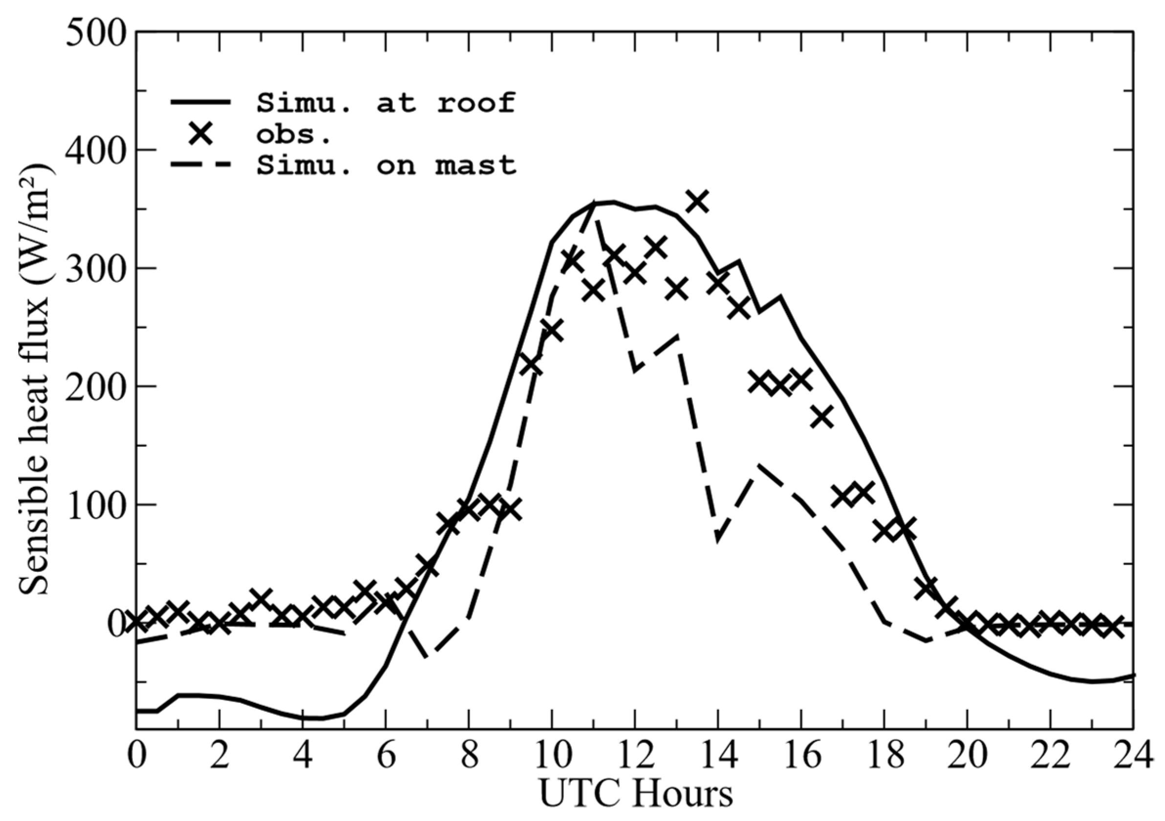
8.5. Sensible Heat Flux $Q_H$

Surface sensible heat flux is the energy exchanged between a surface and the air in the presence of a surface–air thermal gradient. Modelling the sensible heat flux contributes to determine both stratification effects on turbulent transport, and to estimate the surface temperature. At the roof surface, the sensible heat flux $Q_H$ can be parameterized as:

$$Q_H=h_f \left(T_a-T_{sfc}\right),$$

(8)

in which $h_f$ ($\mathrm{W} {\mathrm{m}}^{-2}{\mathrm{K}}^{-1}$) is the heat transfer coefficient and $T_a$ ($\mathrm{K}$) the air temperature.

The sensible heat flux at the surface can be recorded easily in the simulation and be compared to the value measured on the mast computed using the eddy-covariance technique. It can be estimated at the mast level as follows:

$$\overline{w\prime \theta \prime }=K_t\frac{\partial \theta }{\partial z},$$

(9)

where $\overline{w\prime \theta \prime }$ is the potential temperature fluctuation, and eddy diffusivity $K_t$ (${\mathrm{m}}^2 {\mathrm{s}}^{-1}$) by using turbulent viscosity ${\nu }_t$ (${\mathrm{m}}^2 {\mathrm{s}}^{-1}$) and constant turbulent Prandtl number $P{r}_t$ as $K_t={\nu }_t/P{r}_t$. Hence, $Q_H=\rho C_p\overline{w\prime \theta \prime }$.

Figure 17 depicts the comparison between the time evolution of calculated sensible flux at roof surface and the mast observation. At the roof, the difference between observed and calculated values is less than $40 \mathrm{W} {\mathrm{m}}^{-2}$, except for during the night ($45-70 \mathrm{W} {\mathrm{m}}^{-2}$). From midnight to $0700$ UTC, the wind is calm but does not have a zero speed (Figure 5a) and the air temperature varies from $15$ to 19 °C (Figure 5c). The observed sensible flux is very small (cross symbol in Figure 17); this may be due to the fact that the air layer just above the roof has a temperature very close the roof temperature. However, the initialized roof temperature at this position is set to the same value as the measured roof temperature (11.1 °C in Table 1). With a non-zero heat transfer coefficient and a higher air temperature, consequently, negative sensible heat flux is obtained at the roof surface (full line in Figure 17). For the rest of the day the comparison is rather good. At the mast location, reasonable agreement generally exists between calculated and measured values. The differences are more pronounced from 1300 UTC to 1500 UTC. The authors are working on this point in order to better understand the difference. The reason may be due to uncertainty deriving from the measurements and geometries not detailed on the roofs, which has a local influence on the convective flux.

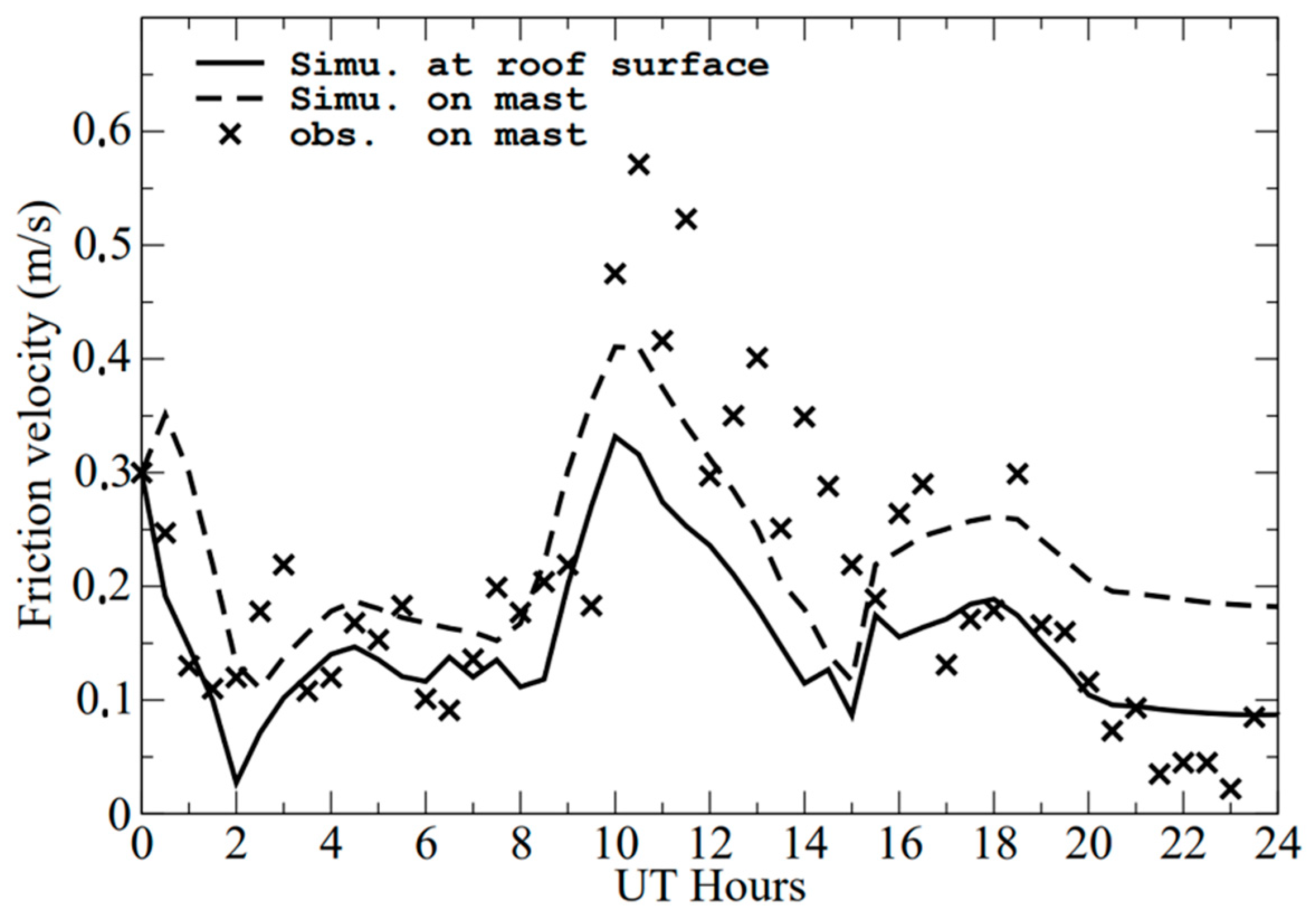
8.6. Model-Observation Comparison of Friction Velocity $u^{*}$

Friction velocity $u^{*}$ ($\mathrm{m} {\mathrm{s}}^{-1}$) was also measured on the mast during the CAPITOUL experiment. The $u^{*}$ at the roof surface is defined by the relation:

$$u^{*}={(\left|{\tau }_w/\rho \right|)}^{1/2},$$

(10)

where ${\tau }_w$ is the Reynolds stress at wall ($\mathrm{N} {\mathrm{m}}^{-2}$) and $\rho$ ($\mathrm{kg} {\mathrm{m}}^{-3}$) the fluid density at the wall.

In order to compare them with the observation on the mast, the kinematic momentum fluxes in the $x$ and $y$ directions ($\overline{u\prime w\prime }$, $\overline{v\prime w\prime }$) are used, and therefore the friction velocity can be evaluated as:

$$u^{*}={({\overline{u\prime w\prime }}^2+{\overline{v\prime w\prime }}^2)}^{1/4},$$

(11)

where $\overline{u\prime w\prime }$ and $\overline{v\prime w\prime }$ are given by:

$$\overline{u\prime w\prime }={\nu }_t\frac{\partial \overline{u}}{\partial z}, \overline{v\prime w\prime }={\nu }_t\frac{\partial \overline{v}}{\partial z},$$

(12)

and ${\nu }_t$ (${\mathrm{m}}^2 {\mathrm{s}}^{-1}$) is the turbulent viscosity given by the $k-\epsilon$ closure.

From Figure 18, it can be seen that the simulated friction velocities are reasonable in terms of magnitude. The modeled friction velocity at roof surface (full line) shows a good agreement with observation when the $u^{*}$ is less than $0.2{ \mathrm{m} \mathrm{s}}^{-1}$. Simulated $u^{*}$ on mast (dashed line) can produce a higher value ($0.4{ \mathrm{m} \mathrm{s}}^{-1}$). It seems that the model overestimates the nighttime ($1800-2400$ UTC) $u^{*}$ on mast. However, estimates of $u^{*}$ from the turbulence measurements by sonic means are known to be rather uncertain, especially when $u^{*}$ is small. The difference between the modeled $u^{*}$ at the roof surface (full line) and at the mast level (dashed line) is due to the different methods of estimation, and numerical errors in the computed gradients.

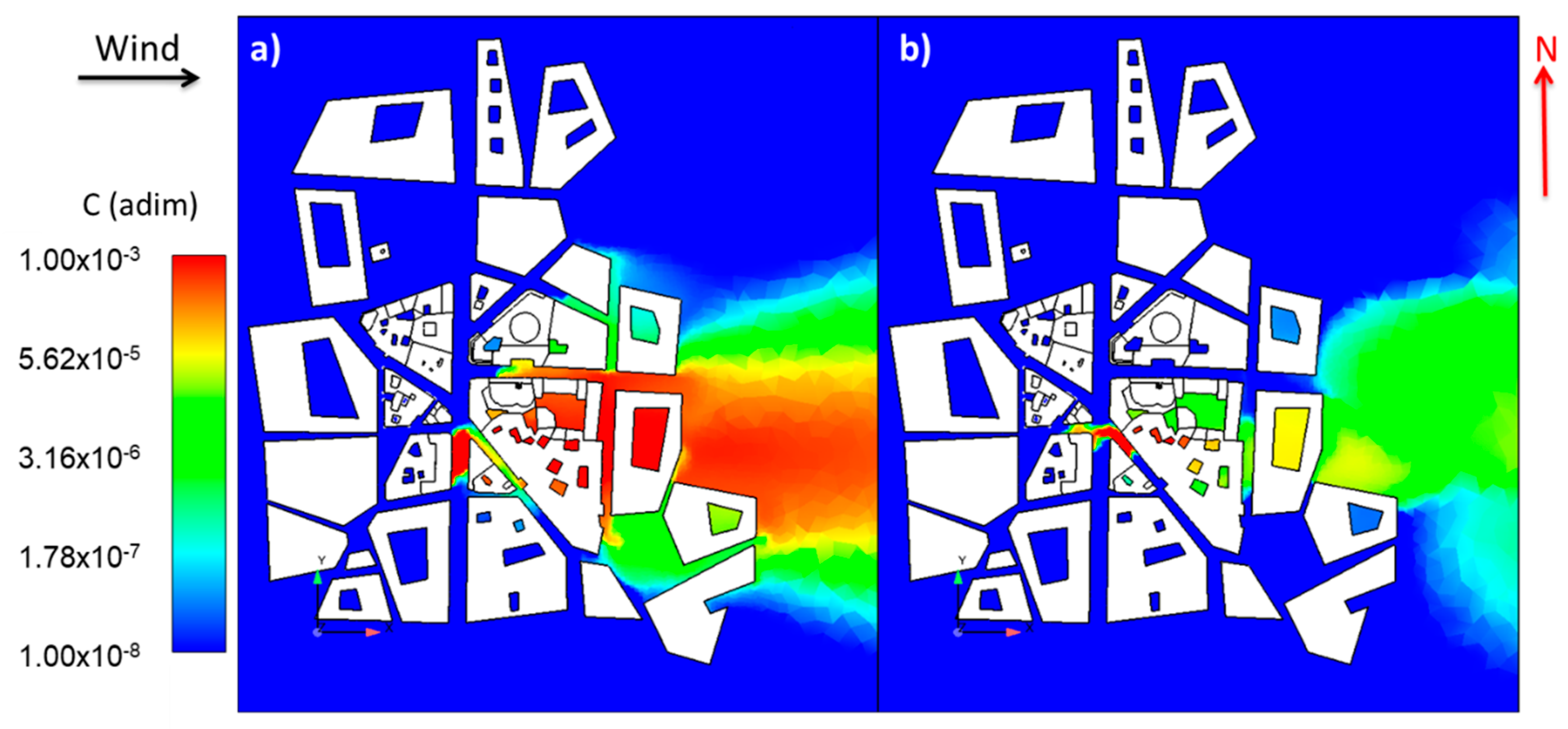
9. Thermal Effects on Pollutant Dispersion

In this section, the thermal effects of buildings on pollutant dispersion are investigated. The meteorological initial and inlet boundary conditions are taken from a neutrally stratified wind profile blowing eastward with a reference wind speed of Uref = 3 m s⁻¹ at 47.5 m height, associated with a neutral potential temperature profile of 22 °C. A passive emission source on the ground is considered that starts at 1000 UTC for a period of 3 h and located as shown in Figure 2a (in the center).

In order to study the contribution of atmospheric radiation on the airflow, two cases were performed: a case with the 3D atmospheric thermo-radiative model coupled to the dynamical one, called hereafter the “thermo-radiative transfer case” and a reference case without heat transfer, i.e., with a neutral stratification of the atmosphere, hereafter called the “neutral case”.

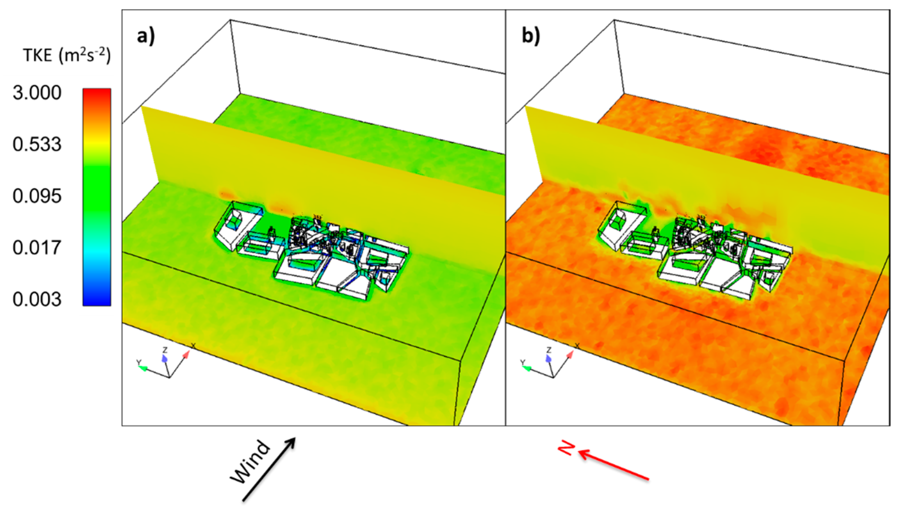
The numerical simulation results are analyzed at the end of the release, when the mean flow in the entire simulated urban canopy reaches a quasi-steady state in the neutral case. Airflow in the urban canopy is composed of very complex vortices rotating in the horizontal and vertical directions. Figure 19a,b shows the Turbulent Kinetic Energy (TKE) fields in the vertical and horizontal cross sections of, respectively, the neutral and thermo-radiative cases. In the neutral case, production of turbulence by the building is confined around the buildings (Figure 19a), the presence of heat transfer (Figure 19b) enhances the TKE both around the buildings and in the whole domain due to a large thermal production, in particular near the roof level.

Figure 20 shows color maps of dimensionless pollution concentration near the ground for two thermal conditions. From the neutral case (Figure 20a), emission from the ground obviously is dispersed by the dominant wind along the west-east direction. Since the wind velocities are reduced dramatically inside the canyons, stagnation areas are formed there. This kind of uneven distribution of wind velocities will definitely influence the pollutant dispersion. Hence in the courtyard pollutants are likely both less diluted and more entrapped than at the roof level (higher courtyard pollutant concentrations).

With thermal transfer condition (Figure 20b), a lower concentration is found downstream; compared to the neutral case, surface heating induces greater dispersion. The courtyard concentration is lower.

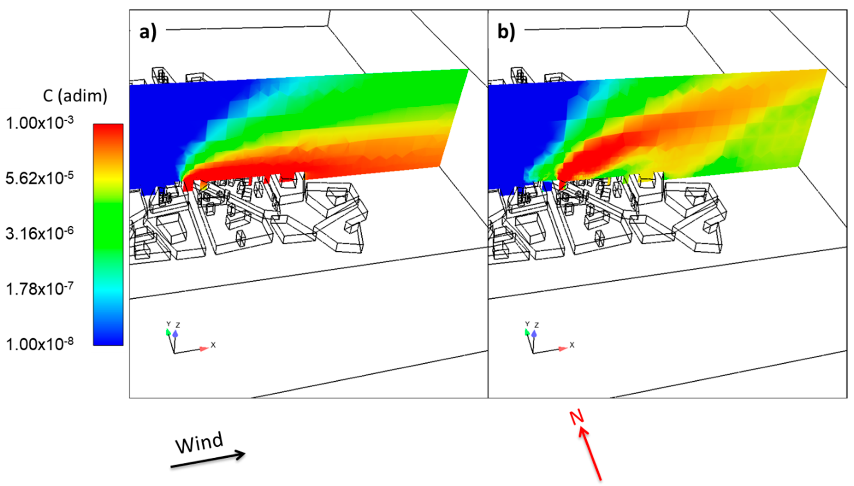
To clarify the change in the dispersion characteristics with changes in thermal condition, the concentration distribution is plotted in a vertical cross section at the released source position in Figure 21. With thermal transfer conditions (Figure 21b), the air temperature is increased which results in an upward motion. Buoyant forces are dominant in this low-wind scenario, as the plume is seen to trend upwards from the point of emission. Moreover, the chosen thermal conditions do lift the plume sufficiently away from the surrounding buildings. Therefore, higher concentrations are found above the road in comparison with the neutral case (Figure 21a). These conclusions are specific to this time of day as, for example, they would be different at nighttime.

10. Conclusions and Perspectives

The energy exchanges in a real city with the atmosphere during the CAPITOUL campaign have been investigated, using new atmospheric radiative and thermal exchange schemes implemented in the open source CFD tool Code_Saturne. A pre-processing of the urban database was performed, including the optimization of the complex geometry, for the creation of a high-quality tetrahedral mesh for this study. The complex thermal parameters have been determined to represent the actual variability of building materials in the district. For example, based on the data from the literature, the authors have separated the building surfaces into four categories of albedo depending on wall colors.

First, the simulations were evaluated in comparison with thermal infrared airborne images from two aircraft flights during the day of 15th July 2004 during the CAPITOUL project. The result shows the importance of taking into account heterogeneities in materials and geometry in order to represent the spatial variability of the temperatures in complex urban areas. Subsequently, we evaluated the coupled dynamic-radiative model with the CAPITOUL field experiment, including a comparison of the measured brightness temperature, sensible flux, diurnal variation in radiative fluxes and statistical differences with hand-held IRT data. Overall, the agreement between measurements and model simulations are fair but can probably be improved in the future with more detailed building information and more refined modelling. For the sensible flux, the model-observation nighttime bias is probably linked to the uncertainty of the estimation on the roof nighttime temperature. Similar explanations can be used for the comparison of the outgoing infrared flux because results are sensitive to the surface temperature. In fact, due to the complex geometries, a comparison of the IR flux in a simple case might be appropriate for understanding the difference and evaluating the model.

Better agreement is obtained for the comparison of the outgoing solar flux at the mast level. However, the difference between the modeled outgoing solar flux at the roof surface and at the mast is still unclear. For the modeled friction velocities, the difficulty mainly appears to capture the extreme values (highest or lowest). Small structures may have an important influence on the computation of local brightness surface temperature, sensible flux and outgoing short- and long-wave radiation. The simulation results show the importance of modelling the details while performing local model-observation comparison. The statistical analysis, while comprehensive, is not exhaustive. Despite the fact that the differences between measured and modeled averaged, median and standard deviation of brightness surface temperature may be significant, such comparison is very useful for a better understanding of the radiative transfer processes in the canopy.

The model results are encouraging and give insight into local surface-atmosphere processes, but further and more rigorous testing has to be performed, especially regarding vertical sensible flux and upward infrared flux. The representativeness of these very localized measurements also has to be assessed.

Using the previously validated simulations, the thermal influence on pollutant dispersion was illustrated by carrying out simulations of a hypothetical pollutant release at ground level in the city center, with and without the thermal effects taken into account. The simulation results show that during the day the warming of the plume by the city center has a strong effect on the calculated concentrations. This illustrates not only the interest of using a CFD code for predicting the dispersion within the complex geometries of urban centers but also that the thermal effects considerably alter the plume shape and the resulting concentrations.

The tool developed in this work can be applied to detailed studies of the local urban climate, and to the study of present conditions and future scenario, such as the densification of housing and the introduction of the green areas or green/white roofs that might be required for future climate studies. It can be used to further assess the street canyon ventilation potential, the possible shading strategies on building surfaces and the influence of both aspects on indoor thermal comfort and air quality. This tool is also well suited to the study of “hot spots” in the air quality of urban centers where the emissions are particularly concentrated and to evaluate the alternatives to mitigate them. It can also contribute to future research and applications in the field of wind engineering in the urban environment when the thermal stratification is of importance. The model results are encouraging and give insight into local surface-atmosphere processes, but further testing and validation has to be performed with other datasets.