Article

Spatiotemporal Variations in Summertime Ground-Level Ozone around Gasoline Stations in Shenzhen between 2014 and 2020

1
School of Sociology, Wuhan University, Wuhan 430072, China
2
School of Philosophy, Zhongnan University of Economics and Law, Wuhan 430073, China
3
School of Sociology, Huazhong University of Science and Technology, Wuhan 430074, China
*
Authors to whom correspondence should be addressed.
Sustainability 2022, 14(12), 7289; https://doi.org/10.3390/su14127289
Submission received: 11 May 2022 / Revised: 10 June 2022 / Accepted: 10 June 2022 / Published: 14 June 2022
(This article belongs to the Special Issue Advances in Applications of Remote Sensing for Urban Sustainability)

Abstract

:
Ground-level ozone has become the primary air pollutant in many urban areas of China. Oil vapor pollution from gasoline stations accelerates the generation of ground-level ozone, especially in densely populated urban areas with high demands for transportation. An accurate spatiotemporal distribution of ground-level ozone concentrations (GOCs) around gasoline stations is urgently needed. However, urban GOCs vary sharply over short distances, increasing the need for GOCs at a high-spatial resolution. Thus, a high-spatial resolution (i.e., 1 km) concentration retrieval model based on the GLM and BME method was developed to obtain the daily spatiotemporal characteristics of GOCs. The hourly ozone records provided by the national air quality monitoring stations and multiple geospatial datasets were used as input data. The model exhibited satisfactory performance (R2 = 0.75, RMSE = 10.86 µg/m3). The derived GOCs show that the ozone levels at gasoline stations and their adjacent areas (1~3 km away from the gasoline stations) were significantly higher than the citywide average level, and this phenomenon gradually eased with the increasing distance from the gasoline stations. The findings indicate that special attention should be given to the prevention and control of ground-level ozone exposure risks in human settlements and activity areas near gasoline stations.

1. Introduction

According to the air quality report released by the Ministry of Ecology and Environment of the People’s Republic of China, ground-level ozone has replaced PM2.5 as the primary pollutant in many areas of China; this situation is particularly prevalent in developed cities and their surrounding areas [1,2]. Repeated exposure to high levels of ground-level ozone can cause symptoms such as coughing, breathing difficulties, decreased lung function, chest tightness and pain, skin wrinkling, nausea and headache, rapid pulse, memory loss, and vision loss [3]. Apart from the adverse effect on human health, ground-level ozone exposure can affect the physiological activities of crops (i.e., photosynthesis and respiration), resulting in reduced crop yields and thus endangering food security [4]. Ground-level ozone also affects air quality and causes climate change [5,6,7]. In recent years, China has actively carried out ground-level ozone pollution prevention and control work and achieved remarkable results [8].
Ground-level ozone is a secondary pollutant formed through photochemical reactions between precursors such as nitrogen oxides (NOx) and atmospheric volatile organic compounds (VOCs) [9,10]. Ground-level ozone concentrations (GOCs) are highly correlated with precursor emissions, and their influencing mechanism varies greatly in different regions [11]. The effect of NOx and VOCs on ozone formation can be described by NOx-limited and VOC-limited regimes, respectively [12]. Compared with the effect of NOx or VOCs, the formation of ground ozone is largely dependent on the VOC/NOx ratio [13]. China has actively promoted management strategies for the emission of ground-level ozone precursors [14]. Obvious results have been achieved for NOx control, but the emission reduction in VOCs has just begun [15]. At present, the emission reduction in VOCs is an important direction of ground-level ozone prevention and control in China [16,17]. The main sources of VOCs are generally oil volatilization and leakage, motor vehicle emissions and the use of liquefied petroleum gasoline [18]. Significantly, gasoline stations, which are the primary source of fuel for cars and motor equipment, emit large amounts of VOCs in the process of refueling and unloading [19,20]. The VOCs will promote the formation of ground-level ozone, posing a potential health threat to people living nearby, especially in densely populated urban areas where there is a high demand for transportation [20,21]. To reduce the adverse effects of ground-level ozone exposure on the health of surrounding residents, it is urgent to clarify the spatial and temporal distribution characteristics of GOCs around gasoline stations.
The main methods for exploring the distribution characteristics of GOCs include ground monitoring and model retrieval [8]. Ground monitoring is the most common atmospheric environment monitoring method; ground monitoring data can provide timely and accurate concentrations. However, the spatial distribution of air quality monitoring stations in China is sparse and uneven; hence, providing concentrations with a continuous spatial distribution is difficult [22]. Therefore, an increasing number of studies have begun to use concentration retrieval models to analyze the spatial and temporal distribution characteristics of GOCs. The retrieval models can not only effectively fill in the blank areas of ground monitoring data, but also provide spatially continuous distribution and long-term change characteristics for GOCs [23].
There are two main concentration retrieval models: the deterministic model and the statistical model. The deterministic model is constructed by using the physical and chemical principles of ground-level ozone formation. However, the spatial resolution of its outputs is low, leading to much uncertainty in simulating complex terrain. In addition, the calculation process of this model is complicated, and its calculation cost is high [20]. The statistical model is established using the statistical correlation between GOCs and influencing factors. In comparison to the deterministic model, the statistical model is more practical for GOC retrievals due to its low computational cost, easy development and high precision [21,22]. Typically, retrieval concentrations at spatial resolutions down to 10 km have been used to characterize the spatiotemporal distribution of GOCs [24]. However, urban GOCs vary sharply over short distances owing to unevenly distributed emission sources, dilution, and physicochemical transformations [25]. To explore the heterogeneity of human exposure and localized pollution hotspots around gasoline stations in urban areas, GOCs with higher (i.e., 1 km) spatial resolution are needed. In our previous study, we designed a hybrid model that combines a generalized linear model (GLM) and a Bayesian maximum entropy (BME) model to retrieve the monthly GOCs at a 1 km spatial resolution [26]. The GLMs are used to predict GOCs at unmonitored sites by using a nonlinear regression framework [27]. The BME models are interpolation methods that assign weights to monitoring values to derive GOCs at unmonitored sites [28]. The combination of a GLM and a BME model exhibited superior performance [29]. On the basis of the hybrid model, we established a retrieval model to obtain the 1 km daily GOCs using hourly in situ ground-level ozone data and multiple geospatial datasets. Then, the spatiotemporal distribution characteristics of GOCs around gasoline stations were discussed to provide a scientific basis and data reference for reducing the health hazards caused by ground-level ozone exposure to surrounding residents.
The remainder of the paper is organized as follows: Section 2 describes the study area and the data preprocessing processes. Section 3 describes the retrieval models and evaluation criteria. The major results are presented in Section 4. The discussions and conclusions are illustrated in Section 5 and Section 6, respectively.

2. Study Area and Data Source

2.1. Study Area

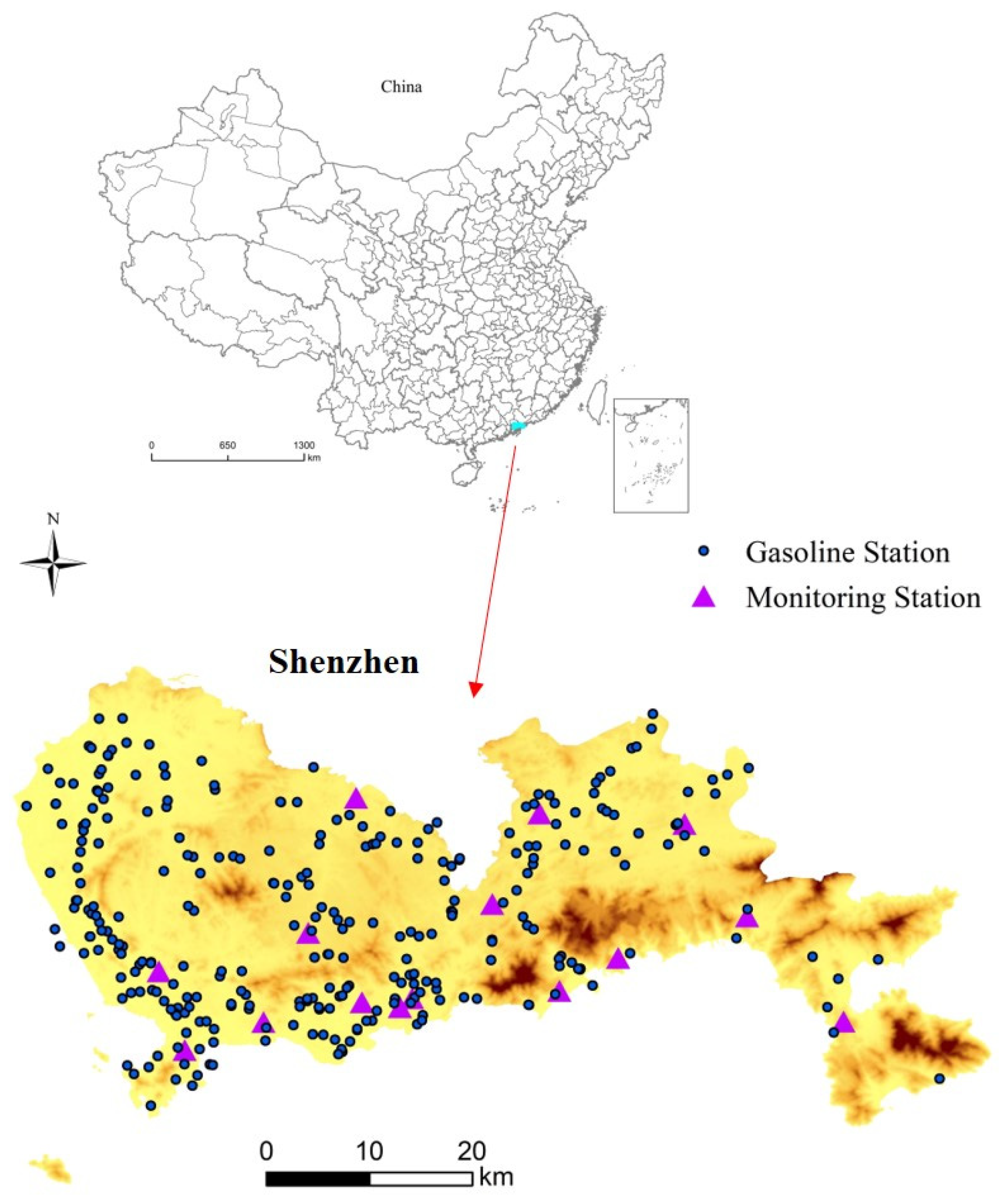
Shenzhen is a megacity in China that has experienced rapid economic development and urbanization, which have been accompanied by representative urban air pollution problems [30,31]. It consists of nine districts with a total area of 1997.47 km2. The national and local governments have adopted a series of measures to reduce air pollution, and the air quality has subsequently improved significantly. However, the situation of ground-level ozone pollution is not positive [15]. Ground-level ozone exposure poses a severe threat to the health of residents [30]. According to the data released by the Municipal Bureau of Ecology and Environment, VOC emissions from gasoline stations are one of the important factors causing ground-level ozone formation, making ground-level ozone become the primary air pollutant in summer in Shenzhen [32,33,34]. As shown in Figure 1, the gasoline stations are mainly concentrated in the western part of Shenzhen, which is also the most densely populated area of the city. In recent years, the number of motor vehicles in Shenzhen has increased sharply. Car ownership in Shenzhen exceeded 3 million by September 2021, leading to rapid growth in gasoline sales. Thus, the Shenzhen Municipal Bureau of Ecology and Environment issued a notice encouraging gasoline stations to adopt preferential economic policies to guide car owners to fuel at night to reduce VOC emissions. The city also strengthened the special detection of oil vapor recovery at gasoline stations to ensure that emissions meet standards.

2.2. In Situ Ground-Level Ozone Data

Hourly ground-level ozone in situ observations from 13 May 2014 to 31 December 2020 were obtained from the China National Environmental Monitoring Center (CNEMC) and used as the input data to the retrieval model. The national monitoring network was set up to monitor air quality in urban areas and their suburbs and became operational in 2013. We used the maximum daily 8 h average ozone (MDA8) from 15 monitoring stations. These stations are roughly evenly distributed throughout Shenzhen (Figure 1). The daily values for each monitoring station were estimated only if at least 18 h of the hourly measurements were available for that day [29,35].

2.3. Multisource Geospatial Datasets

Auxiliary data, such as meteorological variables and aerosols, are often collected for GOC retrieval model establishment [36,37]. Meteorological conditions, including temperature [38,39], relative humidity [40] and precipitation [41], are the main factors affecting GOCs. The GOCs increase when favorable meteorological conditions are present for ground-level ozone formation and accumulation [22,37]. Aerosols are included because they affect the photochemical reaction rates associated with ground-level ozone formation [22,42]. Some human activities (such as transport emissions, coal burning, industrial emissions, etc.) can affect the GOCs [43]. In addition, GOCs are often closely related to economic and social development [44].
According to predictive abilities and data accessibility, multiple multisource geospatial datasets were collected (for details, see Table 1) and resampled to a uniform grid cell (i.e., 1 km × 1 km) by using ArcGIS 10.5, ENVI 4.7 and MATLAB R2014a. The temporal range for these data is from 13 May 2014, to 31 December 2020. The variables numbered 1–10 were obtained from the Modern-Era Retrospective Analysis for Research and Applications, Version 2 (MERRA-2) and resampled by nearest-neighbor interpolation. MERRA-2 is a high-resolution global reanalysis dataset provided by the National Aeronautics and Space Administration (NASA) [45]. This reanalysis dataset has been used in numerous studies, and its quality has been well validated and described in previous studies [22,26,46]. We obtained the land surface temperature data (LST, spatial resolution: 1 km × 1 km) from the Moderate Resolution Imaging Spectroradiometer (MODIS) product MYD11A1 [47].
The road information was extracted from OpenStreetMap (OSM), and the road density (RD) was calculated by using Equation (1).
R D = L e n / A r e a
where L e n is the total length of the major roads within a circular area A r e a with a 1 km radius.
In addition, geolocation information (i.e., longitude (LON) and latitude (LAT)) and temporal information (i.e., day number sequence (DNS)) were also collected. In situ ground-level data and auxiliary data were matched according to their grid cell ID and DNS in the model building and validation process.

3. Methods

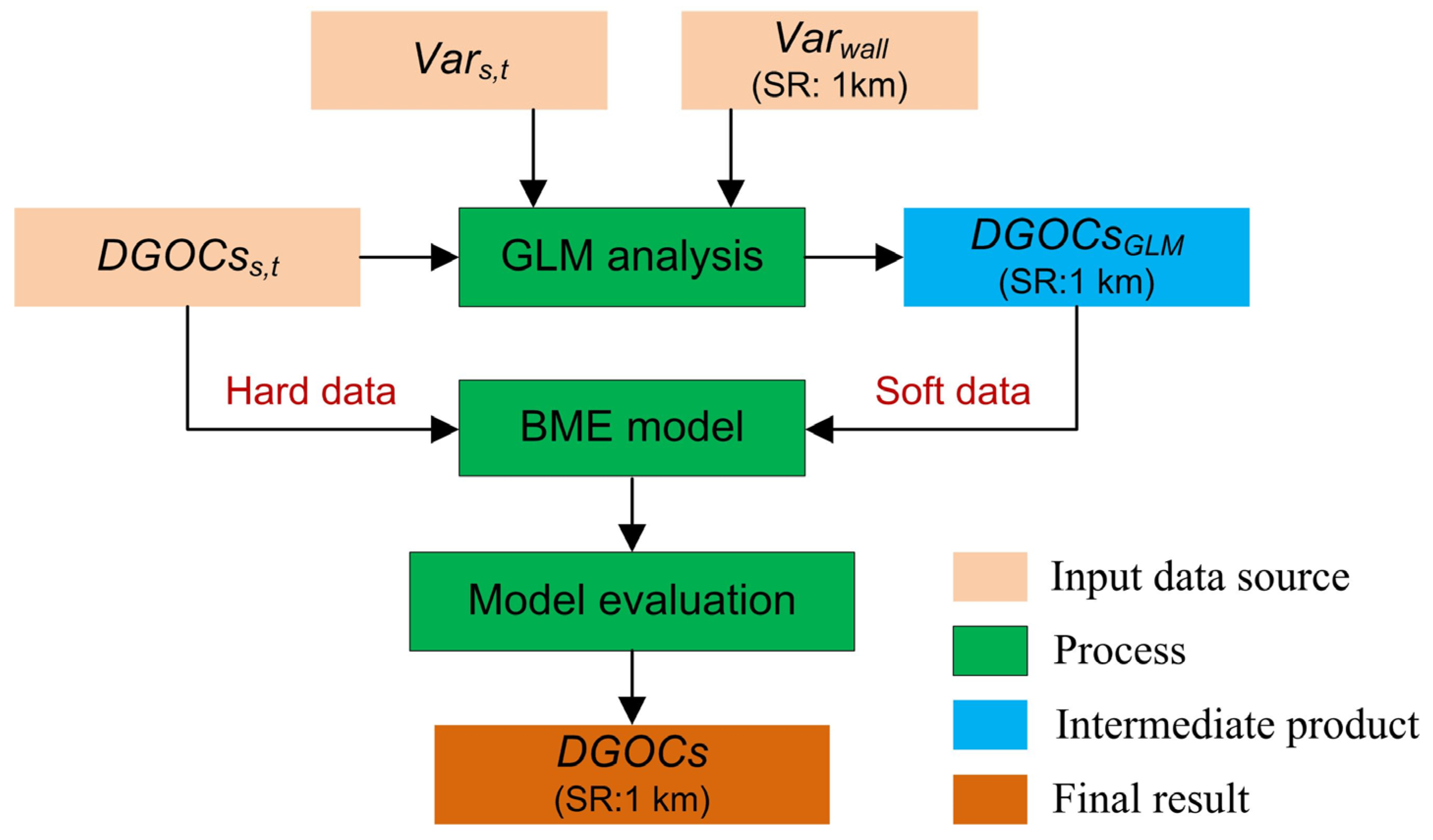
As described in Figure 2, a BME model incorporating the outputs of a GLM was utilized to retrieve the daily GOCs at a 1 km spatial resolution ( D G O C s ). The method consists of two main modules: a GLM analysis and a BME model. The D G O C s s , t and V a r s , t represent the daily average concentrations and auxiliary variables of monitoring site s on day t , respectively, and V a r w a l l represents the high spatial resolution (i.e., 1 km) auxiliary variables. The V a r s , t , V a r w a l l and D G O C s s , t were used as a data source, and the daily GOCs of each eligible grid point ( D G O C s G L M ) was the intermediate product.

3.1. GLM Analysis

A GLM was developed based on the daily average GOCs and auxiliary variables of the monitoring sites [26,27]:
g ( μ ( s ) ) = log μ ( s ) 1 μ ( s ) = j = 0 k X j ( s ) β j
where μ ( s ) is the expected value of daily average GOCs at site s , g ( ) represents the non-linear function, X j ( s ) = ( X j ( s 1 ) , , X j ( s n ) ) represents the auxiliary variables, k   +   1 is the number of regression coefficients β , and β 0 is an intercept.
In total, 15 auxiliary variables were collected for model development (Table 1). The best-fit model is the one that explains the greatest amount of information using the fewest possible variables. Thus, a stepwise regression method based on the Akaike information criterion (AIC) was utilized for variable selection. The smaller the AIC value is, the better the model fit. Any variable whose p-value was higher than 0.05 was excluded. On the basis of V a r w a l l , the daily GOCs of each eligible grid point ( D G O C s G L M ) were estimated by the GLM. The procedure of GLM establishment and variable selection were carried out using Rstudio 3.5.1, an integrated development environment for R software (https://www.rstudio.com/products/rstudio/).

3.2. BME Model

The BME model is a spatiotemporal random field (usually represents as R ) model, as described in Equation (3).
Z ( R ( p ) ) = p f ( p ) d p
where Z is the GOCs at a spatiotemporal point p .
In the general equation of BME model, the posterior probability density function ( f ( p ) ) is as follow [48]:
f ( p ) = f G ( p | p h a r d , p s o f t ) = f G ( p , p h a r d , p s o f t ) f G ( p h a r d , p s o f t )
where f G represents the prior probability density function, p h a r d and p s o f t represent the hard data and soft data, respectively.
Hard data refer to exact measurements without significant uncertainty, which are usually obtained from real-time observation devices and numerical simulations. The hard data we used were the measured daily average GOCs of all eligible site-days ( D G O C s s , t ). Soft data are measurements associated with some known uncertainty, such as imprecise measurements, conclusions derived from empirical intuition judgment, data sequences with missing values, etc. Usually, soft data are expressed in terms of interval values, probability statements and empirical charts [35]. In this paper, the soft data were the daily GOCs of each eligible grid point ( D G O C s G L M ) estimated by the GLM within the study area. There was a total of 4050 possible grid points per day across the study area, and approximately 2,980,800 spatiotemporal points overall. However, soft data were estimated only when all auxiliary variables were available. It was impossible for all the points to be estimated because of missing values. In this study, a total of 27,429 hard data and 130,882 soft data participated in the establishment of the BME model. The BME model was carried out using MATLAB R2014a and the SKES-GUI program, version 1.0.3 [49].

3.3. Model Evaluation

We performed a 10-fold cross-validation to test the predictive ability of the concentration retrieval models. The monitoring datasets were randomly divided into 10 equal-sized subsets. Each of the subsets served exactly once as the source of validation samples. The models were constructed using the monitoring data from the remaining subsets. We then used the trained models to make predictions for the validation samples. This procedure was repeated until each measurement had the corresponding prediction value. The coefficient of determination (R2) and root mean square error (RMSE) were used as the assessment indices.
R 2 = 1 i = 1 m [ y i y ^ i ] 2 ( y i 1 m i = 1 m y i ) 2
R M S E = 1 m i = 1 m ( y i y ^ i ) 2
where y i and y ^ i are the measured concentration and predicted concentration of validation sample i , respectively, and m represents the number of validation samples.

4. Results

4.1. Model Fitting and Evaluation

According to the variable selection procedure described in Section 3.1, RH, BCTP, BCCMASS, OCSMASS, DUSMASS25, SO2SMASS, SO4SMASS, SSSMASS25, LST, LON, LAT and DNS were left in the final GLM (Table 2). The coefficients for BCTP, OCSMASS, SO2SMASS, SO4SMASS and SSSMASS25 were negatively associated with GOCs, whereas RH, BCCMASS, DUSMASS25, LST, LON, LAT and DNS were positively associated with ozone levels. Overall, all predictors had a significant association, except the coefficient of LAT. We also analyzed the positive or negative correlation coefficients between different variables and GOCs. As illustrated in Table 2, LST was the dominant variable and had positive effect on GOCs. RH, BCTP, DUSMASS25, SO2SMASS, SO4SMASS and SSSMASS25 had negative effects on the GOCs, and the other variables had positive effects on the GOCs.
In the BME model, the final covariance model used to fit the measured spatiotemporal covariance of the data consisted of two components. The first component (sill = 0.6) described the majority of the variability; this component consisted of a spherical model in space with a range of approximately 0.01 decimal degrees and an exponential model in time with a range of 40 days. The second component (sill = 0.4) consisted of an exponential model in space with a range of 1.3 decimal degrees and a spherical model in time with a range of 4 days.
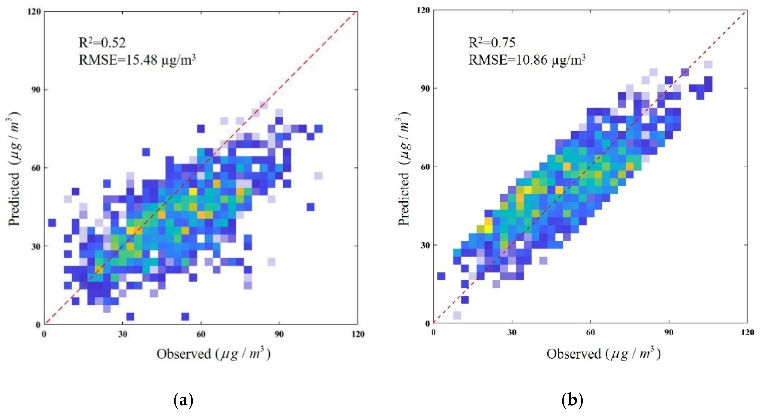
According to the 10-fold cross-validation results (Figure 3), the BME model performed better and had a higher predictive performance (R2 = 0.75, RMSE = 10.86 µg/m3) than the GLM (R2 = 0.52, RMSE = 15.48 µg/m3). We also evaluated the predictive performance of the BME model for each station. The BME model performance exhibited spatial variations, with R2 ranging from 0.54 to 0.80 and RMSE values ranging from 8.68 to 16.39 µg/m3. Given the satisfactory predictive performance, the concentration retrieval model was utilized to generate the daily GOCs at a 1 km spatial resolution.

4.2. Distribution of GOCs in Shenzhen

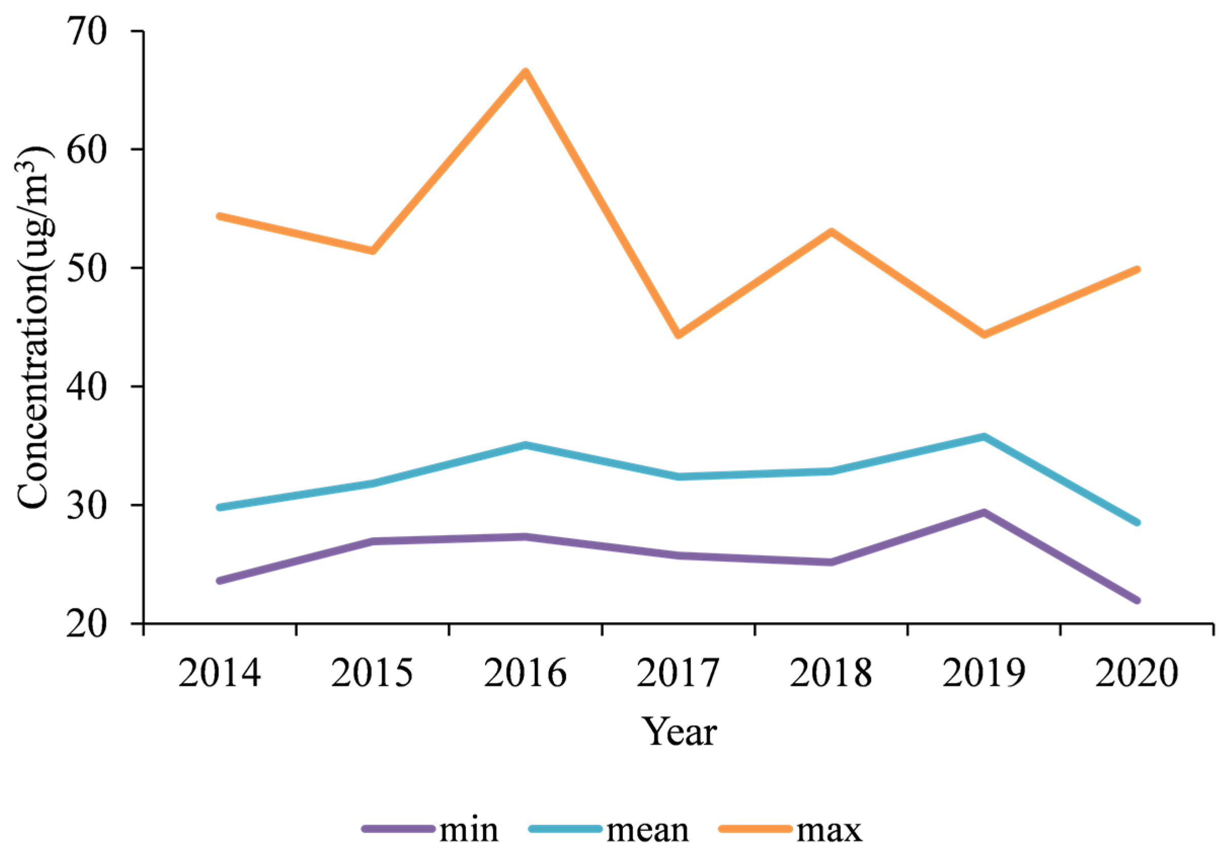
Daily GOCs at a 1 km spatial resolution in Shenzhen during the summertime of 2014 to 2020 were then derived from the concentration retrieval method, and the range of the daily GOCs for summertime of different years was calculated (Figure 4). The daily GOCs from 2014 to 2020 initially increased and then fluctuated before decreasing again. From 2015 to 2019, the mean value of daily GOCs increased with fluctuations, with 35.78 µg/m3 being the highest in 2019. In 2020, the daily GOCs ranged from 21.94 to 49.89 µg/m3, with a mean value of 28.54 µg/m3, which was the lowest of the seven years.
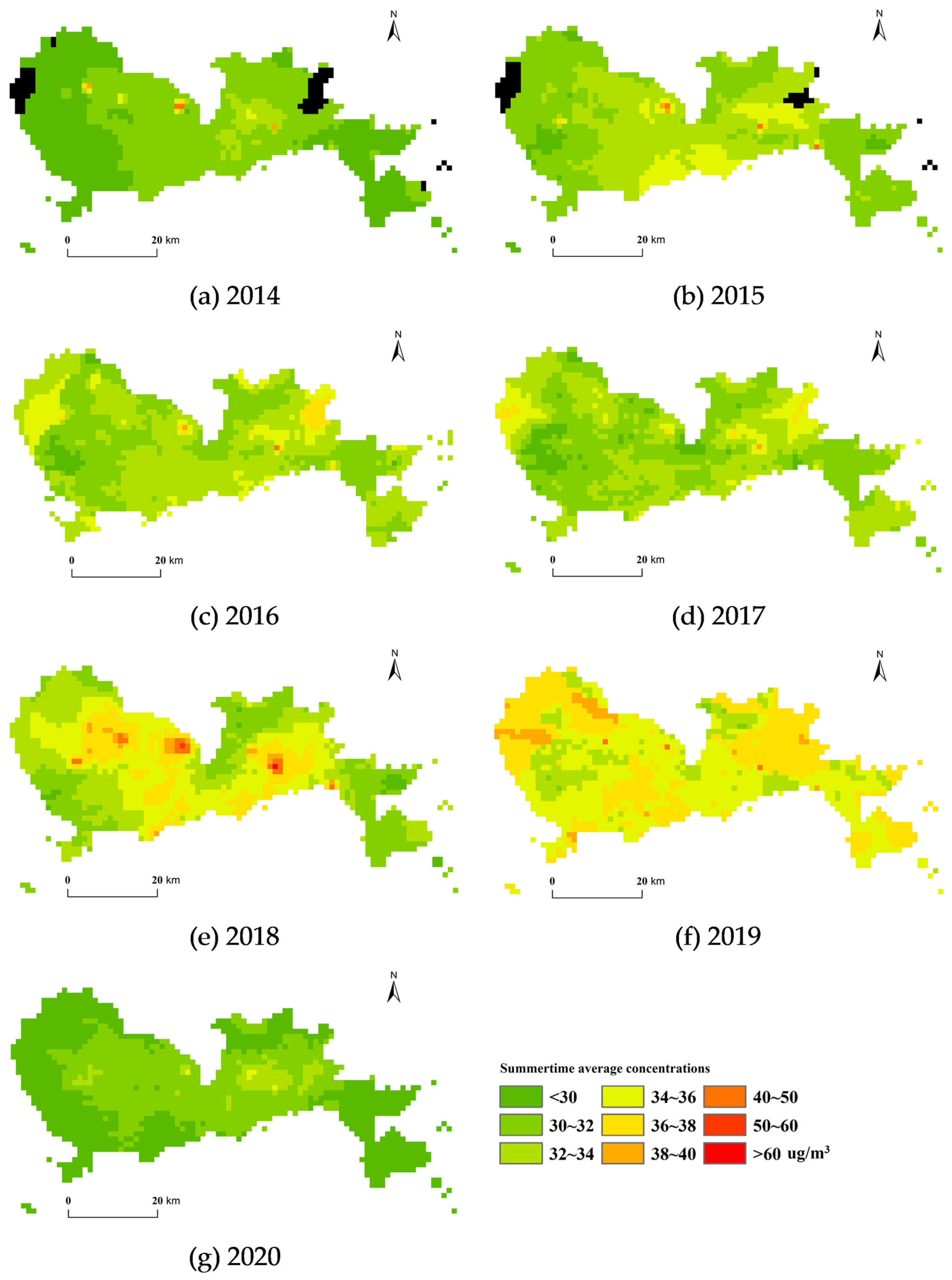
Using the daily GOCs, we calculated the 1 km seasonal average GOCs in Shenzhen for summertime during 2014–2020 (Figure 5). As shown in Figure 5, the summertime average concentrations showed significant spatial heterogeneity and an overall trend of high values in the middle and low values in the west. The areas with the highest summertime average concentrations were mainly concentrated in mid-southern Shenzhen. The summertime average concentration ranged from 28.54 to 35.78 µg/m3 during the study period. The summertime average concentrations mainly showed an upward trend from 2014 to 2019, followed by a downward trend in 2020. They were roughly the same in 2016 and 2017.

4.3. Spatiotemporal Characteristics of GOCs at Gasoline Stations

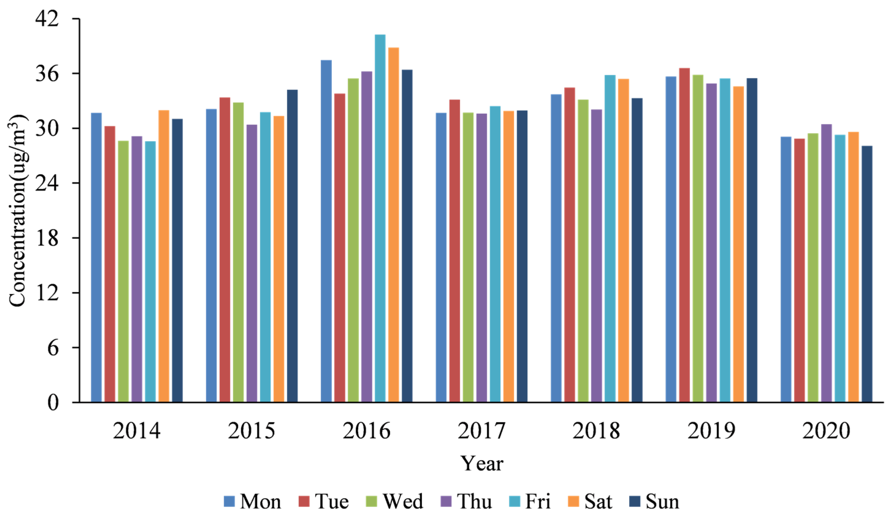
We calculated the daily GOCs at gasoline stations in Shenzhen for the summertime during 2014–2020. The weekly variation in daily GOCs at gasoline stations is illustrated in Figure 6. There is an obvious weekly periodic variation in GOCs at gasoline stations [15]. From 2014 to 2020, the daily GOCs at gasoline stations were higher on Monday, Tuesday, Friday and Saturday. Typically, people travel by car on weekends, driving longer distances than they would normally travel to work. To prepare for the trip, they fill up their fuel tanks (i.e., Friday or Saturday), contributing to high levels of GOCs at gasoline stations. To account for weekend gasoline consumption and weekly commuting trips, people usually fill up on Sunday or during the beginning of the week (i.e., Monday and Tuesday), depending on their needs. These factors help to explain the periodic change in the weekly variation in the daily GOCs [20,50]. In addition, gasoline stations in Shenzhen usually launch preferential activities on Tuesday and Friday to entice drivers to fill up, which also contributes to the relatively high GOCs of gasoline stations on these days. In 2020, Shenzhen launched a special campaign to crack down on the illegal operation of refined oil products and comprehensively monitor the vapor recovery process, thereby improving the quality of oil vapor products [51]. The demand for gasoline also decreased due to the COVID-19 pandemic. With the decrease in oil vapor pollution, the GOCs at gasoline stations also decreased in 2020. In addition to reducing unnecessary outings, people chose to refuel in the middle period of the week (i.e., Wednesday and Thursday) to support daily work and life. These are some of the reasons for the high levels of GOCs at gasoline stations during these days.
The mean values of the daily GOCs at the citywide level and gasoline stations for the study period are illustrated in Figure 7. As shown in Figure 7, the mean value at the citywide level showed an upward trend from 2014 to 2016. It fell in 2017, and then continued to rise until 2019. It reached the lowest value of 28.68 µg/m3 in 2020. According to Figure 7, the mean value of GOCs at gasoline stations in Shenzhen is slightly higher than the citywide average level for summertime 2014–2020, with the exceptions of 2017 and 2019.
A t-test was performed to explore whether there exist significant differences between the mean value of the daily average GOCs at gasoline stations and the citywide level (Table 3). According to the significance tests, the daily average GOCs at gasoline stations are significantly higher than the citywide level for the summertime of different years (except for 2017 and 2019) at a significance level of 5%.
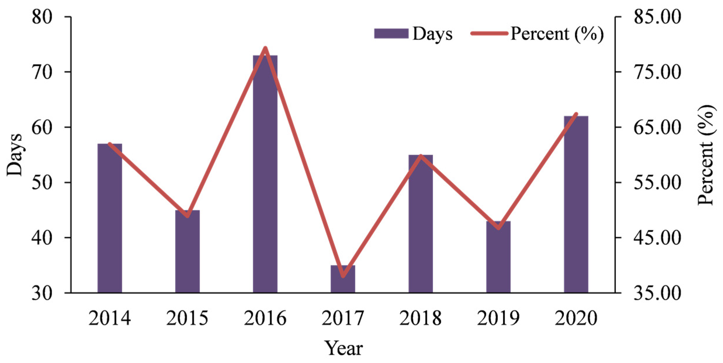
We calculated the percentage of days when the daily average GOCs at the gasoline stations exceeded the city’s average level for the summertime during 2014–2020 (Figure 8). Figure 8 shows that the daily average GOCs at the gasoline stations are higher than the citywide average level on more than half of the summer days for multiple years. Among them, 2016 was the most pronounced, with the daily average GOCs at the gasoline stations exceeding the city’s average level on nearly 80% of the days. In 2017, this phenomenon eased, but the percentage of days when the daily average GOCs at gasoline stations exceeded the city’s daily average level still reached approximately 40%. In 2020, although the overall level of GOCs decreased for both the city overall and the gasoline stations (Figure 7), the former was higher than the latter on nearly 70% of the days. In general, the potential risk caused by ground-level ozone exposure at gasoline stations is more pronounced than the citywide average level.

4.4. Summertime Variations in GOCs around Gasoline Stations Based on Different Radii

To understand the distribution characteristics of GOCs in the vicinity of gasoline stations, we built buffer zones of different radii around each gasoline station and calculated the summertime average GOCs of the corresponding area. As shown in Figure 1, the gasoline stations in Shenzhen are densely distributed, with an average distance of approximately 2.6 km from each other. To reduce the interaction between various gasoline stations, the radius of the buffer zone is set to 1 km, 2 km and 3 km in coordination with the spatial resolution (i.e., 1 km × 1 km) of the derived GOCs. Then, the summertime average GOCs of different buffer zones for different years were calculated (Table 4). As described in Table 4, the summertime average GOCs of the area within 3 km away from the gasoline stations were higher than the citywide level, except in 2017 and 2019. In general, the summertime average GOCs of a buffer zone with a smaller radius was higher than that with a larger radius; these results are basically the same as those in previous studies [20]. However, the ozone formation process is complex, and different influencing factors interact with each other. We cannot attribute the high GOCs to a single factor of oil vapor pollution at gasoline stations.
A t-test was also performed to examine whether there were significant differences between the mean values of the daily GOCs at buffer zones with different radii for multiple years (Table 5). As shown in Table 5, overall, the mean values for buffer zones with smaller radii were significantly higher than those with larger radii. Their differences are quite large for 2016, although they become small in other years for most buffer zone pairs. In addition, there were no significant differences between the values obtained in 2020 and some cases in 2017. Their differences in summertime average concentrations are quite small.

5. Discussion

In recent years, GOCs in many urban areas of China have gradually increased [15,31]. Unlike ozone in the stratosphere, which can absorb solar high-energy ultraviolet radiation, GOCs have adverse effects on human health [1,2]. Repeated exposure to ground-level ozone increases mortality from respiratory diseases [3]. Oil vapor pollution from gasoline stations accelerates the generation of ground-level ozone, especially in densely populated urban areas with a high demand for transportation [52,53]. The rapid increase in car ownership has brought about the continuous growth of gasoline demand; the number of gasoline stations has also increased sharply.
Some gasoline station activities release large amounts of VOCs and promote the formation of ground-level ozone, which has a significant impact on the ambient air quality of gasoline stations and their surrounding areas [19]. One factor is the unloading process of gasoline from tanker trucks to underground storage tanks. The rising level of liquid gasoline displaces the gasoline vapors present in the tank head space. These VOCs can escape and pollute the atmosphere if not captured. The other factor is that when liquid gasoline is pumped from an underground tank into a vehicle’s tank (empty or partially empty), it displaces the vapor in its head space, releasing VOCs [51]. In addition, at gasoline stations, VOCs can also be released from underground storage tanks by “vapor release” [18] and “spillage” [20]. Thus, the temporal and spatial distribution characteristics of GOCs around gasoline stations were studied.
Shenzhen is a large-scale international city with typical characteristics of urban air pollution [30,31]. In this context, this paper has taken Shenzhen as an example to elaborate on relevant scientific issues. The proposed algorithms and models are also applicable to other areas. Empirical results indicated that the hazard of ground-level ozone exposure is higher than the citywide average level from a distance of 1 to 3 km to gasoline stations, and the farther the location from the gasoline stations, the lower the GOCs in general. That is, gasoline stations bring people high quality, convenient, safe and efficient refueling services, but also bring ground-level ozone pollution that cannot be ignored. Thus, special attention should be given to the prevention of ground-level ozone pollution and the supervision of gasoline station:
(1)
Attention should be given to studies on the effects of ground-level ozone pollution on human health in local hot spots, such as gasoline stations. Neighboring residents should reasonably arrange their travel time and activity sphere to reduce the adverse effects caused by ground-level ozone exposure.
(2)
Research on the measurement of VOCs and their effects on ground-level ozone formation in the atmosphere should be strengthened. Future epidemiological studies should focus more on the relationship between ground-level ozone and mortality, such as chronic cardiovascular and respiratory diseases.
(3)
Strict measures are required to control the emissions of ozone precursors (NOx and VOCs), which are mainly from motor vehicle exhaust. In the short term, replacing old cars with newer vehicles or eliminating old cars with subsidies are useful policy strategies. In the long term, developing public transportation to help reduce the use of private cars in major and populous cities is also needed.

6. Conclusions

To analyze the spatiotemporal characteristics of GOCs at gasoline stations and their surrounding areas, a high-spatial resolution (i.e., 1 km) concentration retrieval model was developed by using hourly in situ ground-level ozone data and multiple geospatial datasets. The model exhibited satisfactory performance (R2 = 0.75 and RMSE = 10.86 µg/m3) in retrieving 1 km daily GOCs. The derived GOCs offer valuable information on the spatiotemporal variation characteristics in ground-level ozone at the citywide level and gasoline stations. It finds that the GOCs at gasoline stations and their adjacent areas (1~3 km away from gasoline stations) were significantly higher than the citywide average level, and this phenomenon gradually eased with the increasing distance from the gasoline stations. The findings reveal the potential risk of ground-level ozone exposure to residents’ health around gasoline stations and offer valuable information for preventing ground-level ozone pollution. The determination of the safe distance between gasoline stations and adjacent buildings should consider not only the explosion prevention and fire protection ability of gasoline stations, but also the influence of oil vapor pollution on the surrounding atmosphere. In future work, we will investigate the prediction of long-term GOCs with finer spatial resolution (e.g., 0.1 km) to meet the requirement of assessing ozone pollution hazards around hot spots, such as gasoline stations.

Author Contributions

Conceptualization, Y.M.; methodology, Y.M.; software, Y.M. and X.X.; validation, X.X. and D.X.; formal analysis, D.X.; investigation, Y.M.; resources, D.X.; data curation, Y.M.; writing—original draft preparation, Y.M.; writing—review and editing, X.X.; visualization, Y.M.; supervision, D.X.; project administration, Y.M.; funding acquisition, Y.M. All authors have read and agreed to the published version of the manuscript.

Funding

This research was funded by the National Social Science Foundation of China, grant number 19CSH004.

Conflicts of Interest

The authors declare no conflict of interest.

References

  1. Monks, P.S.; Archibald, A.T.; Colette, A.; Cooper, O.; Coyle, M.; Derwent, R.; Fowler, D.; Granier, C.; Law, K.S.; Mills, G.E.; et al. Tropospheric ozone and its precursors from the urban to the global scale from air quality to short-lived climate forcer. Atmos. Chem. Phys. 2015, 15, 8889–8973. [Google Scholar] [CrossRef] [Green Version]
  2. Brauer, M.; Freedman, G.; Frostad, J.; Van Donkelaar, A.; Martin, R.; Dentener, F.; Van Dingenen, R.; Estep, K.; Amini, H.; Apte, J.; et al. Ambient Air Pollution Exposure Estimation for the Global Burden of Disease 2013. Environ. Sci. Technol. 2015, 50, 79–88. [Google Scholar] [CrossRef] [PubMed]
  3. Avnery, S.; Mauzerall, D.; Liu, J.; Horowitz, L. Global crop yield reductions due to surface ozone exposure: 1. Year 2000 crop production losses and economic damage. Atmos. Environ. 2011, 45, 2284–2296. [Google Scholar] [CrossRef]
  4. Burkey, K.O.; Miller, J.E.; Fiscus, E.L. Assessment of Ambient Ozone Effects on Vegetation Using Snap Bean as a Bioindicator Species. J. Environ. Qual. 2005, 34, 1081–1086. [Google Scholar] [CrossRef] [PubMed]
  5. Chan, C.K.; Yao, X. Air pollution in mega cities in China. Atmos. Environ. 2008, 42, 1–42. [Google Scholar] [CrossRef]
  6. Wang, Y.; Song, Q.; Frei, M.; Shao, Z.; Yang, L. Effects of elevated ozone, carbon dioxide, and the combination of both on the grain quality of Chinese hybrid rice. Environ. Pollut. 2014, 189, 9–17. [Google Scholar] [CrossRef]
  7. Adon, M.; Galy-Lacaux, C.; Delon, C.; Yoboue, V.; Solmon, F.; Tchuente, A.T.K. Dry deposition of nitrogen compounds (NO2, HNO3, NH3), sulfur dioxide and ozone in west and central African ecosystems using the inferential method. Atmos. Chem. Phys. 2013, 13, 11351–11374. [Google Scholar] [CrossRef] [Green Version]
  8. Liu, J.; Wang, L.; Li, M.; Liao, Z.; Sun, Y.; Song, T.; Gao, W.; Wang, Y.; Li, Y.; Ji, D.; et al. Quantifying the impact of synoptic circulation patterns on ozone variability in northern China from April to October 2013–2017. Atmos. Chem. Phys. 2019, 19, 14477–14492. [Google Scholar] [CrossRef] [Green Version]
  9. Yang, L.; Luo, H.; Yuan, Z.; Zheng, J.; Huang, Z.; Li, C.; Lin, X.; Louie, P.K.K.; Chen, D.; Bian, Y. Quantitative impacts of meteorology and precursor emission changes on the long-term trend of ambient ozone over the Pearl River Delta, China, and implications for ozone control strategy. Atmos. Chem. Phys. 2019, 19, 12901–12916. [Google Scholar] [CrossRef] [Green Version]
  10. Li, K.; Jacob, D.J.; Liao, H.; Shen, L.; Zhang, Q.; Bates, K.H. Anthropogenic drivers of 2013-2017 trends in summer surface ozone in China. Proc. Natl. Acad. Sci. USA 2019, 116, 422–427. [Google Scholar] [CrossRef] [Green Version]
  11. Ge, S.; Wang, S.; Xu, Q.; Ho, T. Characterization and sensitivity analysis on ozone pollution over the Beaumont-Port Arthur Area in Texas of USA through source apportionment technologies. Atmos. Res. 2020, 247, 105249. [Google Scholar] [CrossRef]
  12. Yang, G.; Liu, Y.; Li, X. Spatiotemporal distribution of ground-level ozone in China at a city level. Sci. Rep. 2020, 10, 7229. [Google Scholar] [CrossRef] [PubMed]
  13. Pollack, I.B.; Ryerson, T.B.; Trainer, M.; Neuman, J.; Roberts, J.M.; Parrish, D.D. Trends in ozone, its precursors, and related secondary oxidation products in Los Angeles, California: A synthesis of measurements from 1960 to 2010. J. Geophys. Res. Atmos. 2013, 118, 5893–5911. [Google Scholar] [CrossRef]
  14. Cobourn, W.G.; Dolcine, L.; French, M.; Hubbard, M.C. A Comparison of Nonlinear Regression and Neural Network Models for Ground-Level Ozone Forecasting. J. Air Waste Manag. Assoc. 2000, 50, 1999–2009. [Google Scholar] [CrossRef] [PubMed]
  15. Yu, D.; Tan, Z.; Lu, K.; Ma, X.; Li, X.; Chen, S.; Zhu, B.; Lin, L.; Li, Y.; Qiu, P.; et al. An explicit study of local ozone budget and NOx-VOCs sensitivity in Shenzhen China. Atmos. Environ. 2020, 224, 117304. [Google Scholar] [CrossRef]
  16. Wang, T.; Xue, L.; Brimblecombe, P.; Lam, Y.F.; Li, L.; Zhang, L. Ozone pollution in China: A review of concentrations, meteorological influences, chemical precursors, and effects. Sci. Total Environ. 2016, 575, 1582–1596. [Google Scholar] [CrossRef]
  17. Tang, G.; Liu, Y.; Zhang, J.; Liu, B.; Li, Q.; Sun, J.; Wang, Y.; Xuan, Y.; Li, Y.; Pan, J.; et al. Bypassing the NOx titration trap in ozone pollution control in Beijing. Atmos. Res. 2020, 249, 105333. [Google Scholar] [CrossRef]
  18. Zheng, H.; Kong, S.; Xing, X.; Mao, Y.; Hu, T.; Ding, Y.; Li, G.; Liu, D.; Li, S.; Qi, S. Monitoring of volatile organic compounds (VOCs) from an oil and gas station in northwest China for 1 year. Atmos. Chem. Phys. 2018, 18, 4567–4595. [Google Scholar] [CrossRef] [Green Version]
  19. Schifter, I.; Magdaleno, M.; Díaz, L.; Krüger, B.; León, J.; Palmerín, M.E.; Casas, R.; Melgarejo, A.; López-Salinas, E. Contribution of the Gasoline Distribution Cycle to Volatile Organic Compound Emissions in the Metropolitan Area of Mexico City. J. Air Waste Manag. Assoc. 2002, 52, 535–541. [Google Scholar] [CrossRef]
  20. Huy, L.N.; Oanh, N.T.K. Emission control for volatile organic compounds from gasoline stations and implication on ozone-forming potential. Atmos. Pollut. Res. 2020, 11, 87–98. [Google Scholar] [CrossRef]
  21. Zhang, L.; Niu, L. Emission and ozone formation potential analysis of VOCs emitted from fugitive sources. Environ. Eng. 2017, 35, 156. [Google Scholar]
  22. Liu, R.Y.; Ma, Z.W.; Liu, Y.; Shao, Y.C.; Zhao, W.; Bi, J. Spatiotemporal distributions of surface ozone levels in China from 2005 to 2017: A machine learning approach. Environ. Int. 2020, 142, 105823. [Google Scholar] [CrossRef] [PubMed]
  23. Jia, P.; Cao, N.; Yang, S. Real-time hourly ozone prediction system for Yangtze River Delta area using attention based on a sequence to sequence model. Atmos. Environ. 2020, 244, 117917. [Google Scholar] [CrossRef]
  24. Zhan, Y.; Luo, Y.Z.; Deng, X.F.; Grieneisen, M.L.; Zhang, M.H.; Di, B.F. Spatiotemporal prediction of daily ambient ozone levels across China using random forest for human exposure assessment. Environ. Pollut. 2018, 233, 464–473. [Google Scholar] [CrossRef] [PubMed]
  25. Xu, J.; Ma, J.Z.; Zhang, X.L.; Xu, X.B.; Xu, X.F.; Lin, W.L.; Wang, Y.; Meng, W.; Ma, Z.Q. Measurements of ozone and its precursors in Beijing during summertime: Impact of urban plumes on ozone pollution in downwind rural areas. Atmos. Chem. Phys. Discuss. 2011, 11, 12241–12252. [Google Scholar] [CrossRef] [Green Version]
  26. Mei, Y.; Li, J.; Xiang, D.; Zhang, J. When a Generalized Linear Model Meets Bayesian Maximum Entropy: A Novel Spatiotemporal Ground-Level Ozone Concentration Retrieval Method. Remote Sens. 2021, 13, 4324. [Google Scholar] [CrossRef]
  27. Camalier, L.; Cox, W.; Dolwick, P. The effects of meteorology on ozone in urban areas and their use in assessing ozone trends. Atmos. Environ. 2007, 41, 7127–7137. [Google Scholar] [CrossRef]
  28. De Nazelle, A.; Arunachalam, S.; Serre, M.L. Bayesian Maximum Entropy Integration of Ozone Observations and Model Predictions: An Application for Attainment Demonstration in North Carolina. Environ. Sci. Technol. 2010, 44, 5707–5713. [Google Scholar] [CrossRef] [Green Version]
  29. Adam-Poupart, A.; Brand, A.; Fournier, M.; Jerrett, M.; Smargiassi, A. Spatiotemporal Modeling of Ozone Levels in Quebec (Canada): A Comparison of Kriging, Land-Use Regression (LUR), and Combined Bayesian Maximum Entropy–LUR Approaches. Environ. Health Perspect. 2014, 122, 970–976. [Google Scholar] [CrossRef]
  30. Zhang, A.; Lin, J.; Chen, W.; Lin, M.; Lei, C. Spatial–Temporal Distribution Variation of Ground-Level Ozone in China’s Pearl River Delta Metropolitan Region. Int. J. Environ. Res. Public Health 2021, 18, 872. [Google Scholar] [CrossRef]
  31. Jiang, F.; Guo, H.; Wang, T.J.; Cheng, H.R.; Wang, X.; Simpson, I.J.; Ding, A.; Saunders, S.M.; Lam, S.H.M.; Blake, D.R. An ozone episode in the Pearl River Delta: Field observation and model simulation. J. Geophys. Res. Earth Surf. 2010, 115. [Google Scholar] [CrossRef]
  32. Zheng, J.; Zhong, L.; Wang, T.; Louie, P.K.; Li, Z. Ground-level ozone in the Pearl River Delta region: Analysis of data from a recently established regional air quality monitoring network. Atmos. Environ. 2010, 44, 814–823. [Google Scholar] [CrossRef]
  33. Li, J.; Lu, K.; Lv, W.; Li, J.; Zhong, L.; Ou, Y.; Chen, D.; Huang, X.; Zhang, Y. Fast increasing of surface ozone concentrations in Pearl River Delta characterized by a regional air quality monitoring network during 2006–2011. J. Environ. Sci. 2014, 26, 23–36. [Google Scholar] [CrossRef]
  34. Yu, H.-L.; Wang, C.-H. Quantile-Based Bayesian Maximum Entropy Approach for Spatiotemporal Modeling of Ambient Air Quality Levels. Environ. Sci. Technol. 2012, 47, 1416–1424. [Google Scholar] [CrossRef]
  35. Fu, C.; Xu, W.; Dan, L.; Tong, J. Impacts of precursors and meteorological factors on ozone pollution in Hainan province. Environ. Sci. Technol. 2020, 43, 45–50. [Google Scholar]
  36. Li, Y.; Yin, S.; Yu, S.; Bai, L.; Wang, X.; Lu, X.; Ma, S. Characteristics of ozone pollution and the sensitivity to precursors during early summer in central plain, China. J. Environ. Sci. 2020, 99, 354–368. [Google Scholar] [CrossRef]
  37. Sicard, P.; Anav, A.; De Marco, A.; Paoletti, E. Projected global ground-level ozone impacts on vegetation under different emission and climate scenarios. Atmos. Chem. Phys. 2017, 17, 12177–12196. [Google Scholar] [CrossRef] [Green Version]
  38. Spellman, G. An application of artificial neural networks to the prediction of surface ozone concentrations in the United Kingdom. Appl. Geogr. 1999, 19, 123–136. [Google Scholar] [CrossRef]
  39. Abdul-Wahab, S.; Al-Alawi, S. Assessment and prediction of tropospheric ozone concentration levels using artificial neural networks. Environ. Model. Softw. 2002, 17, 219–228. [Google Scholar] [CrossRef]
  40. Biancofiore, F.; Verdecchia, M.; Di Carlo, P.; Tomassetti, B.; Aruffo, E.; Busilacchio, M.; Bianco, S.; Di Tommaso, S.; Colangeli, C. Analysis of surface ozone using a recurrent neural network. Sci. Total Environ. 2015, 514, 379–387. [Google Scholar] [CrossRef]
  41. Huang, R.-J.; Zhang, Y.; Bozzetti, C.; Ho, K.-F.; Cao, J.-J.; Han, Y.; Daellenbach, K.R.; Slowik, J.G.; Platt, S.M.; Canonaco, F.; et al. High secondary aerosol contribution to particulate pollution during haze events in China. Nature 2014, 514, 218–222. [Google Scholar] [CrossRef] [PubMed] [Green Version]
  42. Xue, L.K.; Wang, T.; Gao, J.; Ding, A.J.; Zhou, X.H.; Blake, D.R.; Wang, X.F.; Saunders, S.M.; Fan, S.J.; Zuo, H.C.; et al. Ground-level ozone in four Chinese cities: Precursors, regional transport and heterogeneous processes. Atmos. Chem. Phys. 2014, 14, 13175–13188. [Google Scholar] [CrossRef] [Green Version]
  43. Cheng, L.; Wang, S.; Gong, Z.; Li, H.; Yang, Q.; Wang, Y. Regionalization based on spatial and seasonal variation in ground-level ozone concentrations across China. J. Environ. Sci. 2018, 67, 179–190. [Google Scholar] [CrossRef] [PubMed] [Green Version]
  44. Gelaro, R.; McCarty, W.; Suárez, M.J.; Todling, R.; Molod, A.; Takacs, L.; Randles, C.A.; Darmenov, A.; Bosilovich, M.G.; Reichle, R.; et al. The Modern-Era Retrospective Analysis for Research and Applications, Version 2 (MERRA-2). J. Clim. 2017, 30, 5419–5454. [Google Scholar] [CrossRef]
  45. Li, G.; Bei, N.; Cao, J.; Wu, J.; Long, X.; Feng, T.; Dai, W.; Liu, S.; Zhang, Q.; Tie, X. Widespread and persistent ozone pollution in eastern China during the non-winter season of 2015: Observations and source attributions. Atmos. Chem. Phys. 2017, 17, 2759–2774. [Google Scholar] [CrossRef] [Green Version]
  46. Duan, S.-B.; Li, Z.-L.; Leng, P. A framework for the retrieval of all-weather land surface temperature at a high spatial resolution from polar-orbiting thermal infrared and passive microwave data. Remote Sens. Environ. 2017, 195, 107–117. [Google Scholar] [CrossRef]
  47. Yang, Y.; Christakos, G. Spatiotemporal characterization of ambient PM2.5 concentrations in Shandong province (China). Environ. Sci. Technol. 2015, 49, 13431–13438. [Google Scholar] [CrossRef]
  48. Yu, H.-L.; Kolovos, A.; Christakos, G.; Chen, J.-C.; Warmerdam, S.; Dev, B. Interactive spatiotemporal modelling of health systems: The SEKS–GUI framework. Stoch. Hydrol. Hydraul. 2007, 21, 555–572. [Google Scholar] [CrossRef]
  49. Lu, X.; Hong, J.; Zhang, L.; Cooper, O.R.; Schultz, M.G.; Xu, X.; Wang, T.; Gao, M.; Zhao, Y.; Zhang, Y. Severe surface ozone pollution in China: A global perspective. Environ. Sci. Technol. Lett. 2018, 5, 487–494. [Google Scholar] [CrossRef]
  50. Wang, Y.H.; Hu, B.; Ji, D.S.; Liu, Z.R.; Tang, G.Q.; Xin, J.Y.; Zhang, H.X.; Song, T.; Wang, L.L.; Gao, W.K.; et al. Ozone weekend effects in the Beijing-Tianjin-Hebei metropolitan area, China. Atmos. Chem. Phys. 2014, 14, 2419–2429. [Google Scholar] [CrossRef] [Green Version]
  51. Yu, G.; Lin, L.; Xia, S.; Zhu, B.; Huang, X. The characteristics of VOCs and ozone formation sensitivity in a typical industrial area in Shenzhen. China Environ. Sci. 2022, 42, 1994–2001. (In Chinese) [Google Scholar]
  52. Meng, X.Y.; Wang, R.B.; Du, L.; Li, J.; Yu, Y. The characters of variation of ozone in experimental cities. Environ. Monit. China 2013, 29, 64–70. [Google Scholar]
  53. Yamamoto, Y.; Kambe, Y.; Yamada, H.; Tonokura, K. Measurement of Volatile Organic Compounds in Vehicle Exhaust Using Single-Photon Ionization Time-of-Flight Mass Spectrometry. Anal. Sci. 2012, 28, 385. [Google Scholar] [CrossRef] [PubMed] [Green Version]
Figure 1. Locations of gasoline stations and air quality monitoring stations in Shenzhen.
Sustainability 14 07289 g001
Figure 2. Flow chart of the concentration retrieval method (SR: spatial resolution).
Sustainability 14 07289 g002
Figure 3. Density scatter plots of measurements and predictions for (a) GLM and (b) BME model (color bar represents the frequency of points).
Sustainability 14 07289 g003
Figure 4. Range of daily GOCs in Shenzhen for the summertime of 2014–2019.
Sustainability 14 07289 g004
Figure 5. Summertime average GOCs at a 1 km spatial resolution in Shenzhen during 2014–2020 ((ag) represent the years of 2014 to 2020, the black color represents NaN data).
Sustainability 14 07289 g005
Figure 6. Weekly variation in daily average GOCs at gasoline stations for the summertime during 2014–2020.
Sustainability 14 07289 g006
Figure 7. The mean value of the daily GOCs at the citywide level and gasoline stations in Shenzhen for summertime during 2014–2020.
Sustainability 14 07289 g007
Figure 8. Percentage of days when the daily average GOCs at the gasoline stations exceeded the city’s average level in Shenzhen for summertime during 2014–2020.
Sustainability 14 07289 g008
Table 1. List of auxiliary variables.
NumberAbbreviationDescriptionUnitSpatial
Resolution
Temporal
Resolution
1RHrelative humidity after moisture10.667° × 0.5°Day
2BCTPbias corrected total precipitationkgm−2 s−10.667° × 0.5°Day
3BCCMASSblack carbon column mass densitykgm−20.667° × 0.5°Day
4OCSMASSorganic carbon surface mass concentrationkgm−20.667° × 0.5°Day
5DUSMASS25dust surface mass concentration-PM2.5kgm−30.667° × 0.5°Day
6SO2SMASSSO2 surface mass concentrationkgm−30.667° × 0.5°Day
7SO4SMASSSO4 surface mass concentrationkgm−30.667° × 0.5°Day
8SSSMASS25sea salt column mass density-PM2.5kgm−30.667° × 0.5°Day
9PGENTOTtotal column production of precipitationkgm−2 s−10.667° × 0.5°Day
10QV2M2-m specific humiditykg kg−10.667° × 0.5°Day
11LSTland surface temperature° C1 km × 1 kmDay
12RDroad densitykm/km2PolylineYear
13LONlongitude°NANA
14LATlatitude°NANA
15DNSday number sequenceNANANA
Table 2. Summary of the information for the GLM (confidence level = 95%).
NumberVariableCoefficientConfidential IntervalCorrelation Coefficient
1Constant3.49[3.45, 3.52]
2RH0.12[0.08, 0.16]−0.01
3BCTP−1.68[−1.90, −1.47]−0.05
4BCCMASS4.42[4.18, 4.65]0.02
5OCSMASS−4.39[−4.64, −4.13]0.01
6DUSMASS250.49[0.43, 0.55]−0.02
7SO2SMASS−0.45[−0.51, −0.39]−0.16
8SO4SMASS−0.18[−0.22, −0.13]−0.12
9SSSMASS25−0.35[−0.40, −0.30]−0.13
10LST1.30[1.26, 1.35]0.26
11LON0.10[0.08, 0.13]0.02
12LAT0.05[0.03, 0.07]0.02
13DNS0.11[0.10, 0.13]0.06
Table 3. Differences between the mean values of the daily GOCs at the gasoline stations and the citywide level for different years (*: significant at a level of 5%).
Year2014201520162017201820192020
Difference0.38 *0.48 *1.76 *−0.301.15 *−0.26−0.63 *
Table 4. Summertime average GOCs of buffer zones with different radii during 2014–2020 (µg/m3).
2014201520162017201820192020
Radius1 km30.2432.3536.8832.1233.9835.6829.31
2 km30.2332.3436.8032.1033.9335.6529.33
3 km30.1832.3136.7232.0933.8835.6329.35
Citywide level29.8131.8435.1832.4232.8935.8328.69
Table 5. Summertime average concentration differences between alternative buffer zones with different radii (*: significant at a level of 5%): (I) 1 km, (II) 2 km, and (III) 3 km.
Buffer Zone PairsYear
2014201520162017201820192020
I versus II0.01 *0.01 *0.08 *0.02 *0.05 *0.03 *−0.02
I versus III0.06 *0.04 *0.16 *0.030.10 *0.05 *−0.04
II versus III0.05 *0.03 *0.08 *0.010.05 *0.02−0.02
Publisher’s Note: MDPI stays neutral with regard to jurisdictional claims in published maps and institutional affiliations.