Towards Safe and Sustainable Autonomous Vehicles Using Environmentally-Friendly Criticality Metrics

Abstract

This paper presents an analysis of several criticality metrics used for evaluating the safety of Autonomous Vehicles (AVs) and also proposes environmentally friendly metrics with the scope of facilitating their selection by future researchers who want to evaluate both the safety and environmental impact of AVs. Regarding this, first, we investigate whether existing criticality metrics are applicable as a reward component in Reinforcement Learning (RL), which is a popular learning framework for training autonomous systems. Second, we propose environmentally friendly metrics that take into consideration the environmental impact by measuring the CO₂ emissions of traditional vehicles as well as measuring the motor power used by electric vehicles. Third, we discuss the usefulness of using criticality metrics for Artificial Intelligence (AI) training. Finally, we apply a selected number of criticality metrics as RL reward component in a simple simulated car-following scenario. More exactly, we applied them together in an RL task, with the objective of learning a policy for following a lead vehicle that suddenly stops at two different opportunities. As demonstrated by our experimental results, this work serves as an example for the research community of applying metrics both as reward components in RL and as measures of the safety and environmental impact of AVs.

1. Introduction

The research interest in the domain of AVs, especially regarding their safety, has grown exponentially in the last few years. This is mainly due to recent advancements in the field of AI, especially regarding deep RL algorithms, which are showing promising results when implemented in AI components found in AVs, especially when combined with prior knowledge [1].

Concerning traffic scenarios, the safety of all traffic participants is considered to be the most important aspect on which the researchers should focus, this being especially reflected by projects such as VVM—Verification and Validation Methods for Automated Vehicles Level 4 and 5 [2], SET Level—Simulation-Based Development and Testing of Automated Driving [3], as well as KI Wissen—Automotive AI Powered by Knowledge [4], all three projects being funded by the German Federal Ministry for Economic Affairs and Climate Action. In addition to these, many other projects of the VDA Leitinitiative autonomous and connected driving [5] bring together various research partners from the industry and academia to solve challenging and contemporary research problems related to the AV domain, emphasizing the relevance of criticality and safety in traffic.

With regards to the meaning of criticality, despite the existent ambiguity regarding its definition in both industry and academia, for an easier understanding of its meaning in the context of this paper, we follow the definition given by the work in [6] (Def. I), namely: “the combined risk of the involved actors when the traffic situation is continued”.

Regarding this, to assess how critical a traffic situation is, literature focuses on the use of so-called criticality metrics for automated driving [7,8]. However, because AVs are operating in a complex traffic environment where a high number of actors are present, such as AVs, non-AVs, and pedestrians, to name only a few, it is imperative to not only identify the suitable criticality metrics that can mitigate dangerous situations as it is currently done in the literature [7,8] but also to implement and evaluate them efficiently regarding their environmental impact as well.

This is of high importance, especially when the transportation sector is known to be a key contributor to climate change, accounting for more than 35% of carbon dioxide emissions in the United States alone [9]. It is therefore imperative that existent and future researchers do not only use existent metrics that can evaluate critical situations in traffic, but also make efforts in proposing novel environmentally friendly criticality metrics that can be used to evaluate the AV’s impact on the environment and economy as well. A recent effort in this direction is made by a new global initiative that tries to catalyze impactful research work at the intersection of climate change and machine learning such as the work of the Climate Change AI [10] organization as well as in recent works that try to encourage researchers to power and evaluate their deep learning-based systems using green energy [11,12].

Autonomous systems can be rule-based, i.e., there is a pre-defined deterministic policy that decides which action the AV should take in which situation (e.g., regarding distances to other vehicles and relative velocities), but the growing potential of deep learning leads to AVs trained with AI or even a combination of rule- and AI-based components as intended by the KI Wissen project [4]. The AI-based training of AVs is usually based on RL. As the criticality metrics evaluate the safety of the AV, it is hence a logical step to respect those metrics already in the training process which, for RL, can be done by reward shaping, i.e., integrating additional (criticality-related) terms into the reward function that acts as target function during training.

Therefore, in this paper, we present an analysis of several criticality metrics, mainly the ones already collected in [7,8], in order to determine whether they can be applied as reward components in AI training by RL to easily facilitate their selection for criticality assessment in the context of AV safety evaluation. To this end, the used criticality metrics must satisfy the property that the desired behaviour, represented by an optimal policy, is flagged as optimal by the respective metrics. It is important to mention that our analysis is a special case of the proposed application, as per the “Objective function” in [7] (Section 3.1.1). This is done, first, on the base of the formula and secondly, via an evaluation of selected criticality metrics. Additionally, we propose to combine these metrics with what we call “environmentally friendly metrics” in order to take the CO₂ footprint explicitly into account.

Furthermore, due to recent emergent paradigms, such as Green AI [13], which encourage researchers to move towards more sustainable methods that are environmentally friendly and inclusive, we also propose several environmentally friendly metrics that are used to create an environmentally friendly criticality metric, which is suitable for evaluating a critical scenario not only regarding safety but also regarding the environmental impact in a car-following scenario.

Our main contributions are as follows: (i) an analysis of the existing criticality metrics in terms of applicability as a reward component and how they can be used to learn towards safe and desired behavior; (ii) the integration of existing criticality metrics as reward components in RL and of emission estimations into the criticality metrics framework; (iii) an investigation of the suitability of the criticality metrics for AI training; (iv) illustrative simulations of the metrics applied in a car-following scenario.

The paper is organized as follows. In Section 2, we present the related work. Section 3 details the analysis of several criticality metrics, as well as adaptions allowing for their possible applicability as a reward component. Section 4 presents the proposed environmentally friendly criticality metrics. Section 5 presents our contribution regarding the usage of criticality metrics for AI training. In Section 6 we present the application of the metrics. Finally, in Section 7, we present the conclusions, limitations and future work of this paper.

2. Related Work

An extensive overview of criticality metrics in autonomous driving has been given by Westhofen et al. in [7,8]. The usage of criticality metrics is not restricted to the evaluation of traffic scenarios, but can be extended to the training of autonomous driving agents by integrating suitable metrics into the reward function, whereas such an application has already been proposed in [7] and is analyzed here in depth regarding general requirements of such metrics for the use case of RL. This technique is called reward shaping and allows for prior knowledge to be included in the training, as seen in [14]. Three of these criticality metrics, namely Headway (HW), Time Headway (THW), and Deceleration to Safety Time (DST), were implemented and tested in an Adaptive Cruise Control (ACC) use case, as detailed by the authors of [1]. In their work, the authors have shown that different RL models can be evaluated for the ACC use case using these metrics; however, the DST metric, at the very least, does not coincide with the supposed objective of this function.

The ecological impact of autonomous driving has been discussed in many works, such as the ones in [15,16,17,18,19]. These works do not only consider fuel consumption or emissions but also analyze the socio-ecological aspects, like a higher driving demand if AVs are available, or indirect implications, like reduced land use due to optimized parking. Moreover, the work in [20] proposes a model for estimating the emissions and evaluating it in different scenarios with respect to, for example, the relative part of AVs in the traffic. The authors of [21] propose a model for CO${}_2$ emission estimation. The power consumption of electric vehicles was also measured by [22,23,24].

The cited references generally consider fuel consumption and emissions for evaluation. These measures can be seen as environmentally friendly metrics, which have already been used for AI training. For example, the authors of [25] train a deep RL model that is encouraged to minimize emissions, and the authors of [26] proposed a deep RL controller based on a partially observed Markov Decision Problem for connected vehicles so that eco-driving is encouraged where battery state-of-charge and safety aspects (e.g., speed limits or safety distances) are integrated into the model. Additionally, the work in [27] presents an extensive overview of eco-driving RL papers where the reward function is nearly always state-of-charge or fuel consumption. The authors of [28] propose a hybrid RL strategy where conflicting goals such as saving energy and accelerating are captured by a long-short-term reward (LSTR). To not let energy-saving jeopardize safety, the acceleration energy is only penalized for accelerations, not for decelerations. The reward function also consists of a green-pass reward term, which essentially encourages reaching the stopping line of an intersection when the traffic light is green (i.e., driving forward-looking). Some of these references not only focus on carbon dioxide emissions but also consider, for example, carbon monoxide, methane, or nitrogen oxides. Besides training AVs, ecological aspects are also taken into consideration regarding traffic system controls [29].

3. Applicability Analysis of Criticality Metrics

In the following, we present an analysis of several existing criticality metrics. We have mostly made use of the excellent overview and detailed presentation in Westhofen et al. [7] and the supplementary material [8]. While Westhofen et al. put a lot of emphasis on an abstract, unifying representation of the metrics, we concretized most of the metrics to the case of a track-/car-following scenario. In particular, this means that we generally view an actor’s position as a one-dimensional quantity, $p_i$, that measures the progress of actor i from an arbitrary reference point relative to a given route. All actor positions refer to the same reference point, so, for every two actors, i and j, it can be effectively decided whether actor i is in front of actor j ($p_i>p_j$), the other way around ($p_i<p_j$), or whether both actors are in the same position ($p_i=p_j$), which usually indicates the presence of a collision. Only in a few cases do we consider the position of the actor i as a vector quantity, $p_i$, in the two-dimensional plane.

As for the notation in the subsequent parts, please see the Abbreviations and Nomenclature sections where the most frequent abbreviations and symbols used in this paper are presented. Note that state variables like position ($p_i\left(t\right)$), velocity ($v_i\left(t\right)$) and acceleration ($a_i\left(t\right)$), specific to actor i, are functions over time. The current time of a scene is denoted by $t_0$, and if we refer to a state variable at time $t_0$, we often omit the time parameter; i.e., we briefly write $p_i$ instead of $p_i\left(t_0\right)$.

In general, criticality metrics refer to an underlying prediction model (PM) to predict the future evolution of the actual traffic scene. While in the standard literature such predictive models are fixed in the definition of the metrics, we benefit from the preliminary work by Westhofen et al. [7], who have freed many metrics from the fixed predictive models and made them a flexible component of the metrics. Often, a prediction model can be obtained from a dynamic motion model (DMM) that approximates the agent’s future position. If, for example, in the definition of a metric, the position function $p_i\left(t\right)$ is applied to future time points, then it is mandatory to specify a DMM for an in-situ computation. Typical DMMs arise from the assumption of constant velocity ($p_i(t_0+t)=p_i+v_{i}t$) or constant acceleration ($p_i(t_0+t)=p_i+v_{i}t+\frac{1}{2}{a}_i{t}^2$).

In AI training, criticality metrics can be used as penalty terms, for example, as negative reward components in RL. More precisely, RL training corresponds to (approximately) solving a so-called Markov decision process (MDP), represented by a tuple $(\mathcal{S},\mathcal{A},T,r,\gamma )$ (e.g., [30]) for the state space $\mathcal{S}$, the action space $\mathcal{A}$; and a transition model $T:\mathcal{S}\times \mathcal{A}\times \mathcal{S}\to [0,1]$ where $T(s,a,s^{\prime })=P\left(s^{\prime }\right|a,s)$ is the transition probability from state s to state $s^{\prime }$ if action a has been selected by the ego agent. The ego agent’s behaviour is described by a policy $\pi :\mathcal{S}\times \mathcal{A}\to [0,1]$ where $\pi (s,a)=P\left(a\right|s)$ describes the probability that the ego agent selects action a in state s. $\gamma \in [0,1]$ is a discount factor and $r:\mathcal{S}\times \mathcal{A}\to \mathbb{R}$ is a reward function which returns a real-valued feedback for the ego agent’s decision. This reward function can consist of different reward components that aim to encourage or discourage certain behaviours. RL training is an iterative process where one starts with some initial policy. For given states, actions are selected by this policy and some time steps are played out using the given transition model, up to some finite horizon. Then, the resulting trajectories are evaluated by the reward function so that the policy is updated accordingly in the sense that actions that were appropriate for the given states, therefore leading to high rewards, are encouraged in the future by modifying the current policy.

The agent, therefore, successively learns to select appropriate actions, resulting in maneuvers that are not critical or in which criticality is sufficiently low, evaluating the selected metrics. As an action usually only considers acceleration/deceleration and changing the heading angle, parameters that cannot be influenced by the agent like payloads; the length of the vehicle; or, generally, its structure, could only implicitly be considered when computing the rewards; e.g., higher payloads can be integrated into the computation of the braking distance. These parameters often correspond to passive safety and optimizing them is part of the manufacturing process [31], but it does not correspond to the scope of this work. Note that, due to the playout of the trajectories in RL training, one has to be careful considering metrics like TTC where one searches for a particular timestep in the future where the vehicles would collide. If a collision did not happen in the played-out trajectories, one could empirically set TTC at least to ∞, but that would not fully reflect its definition. Overall, the relationship between the prediction models of the metrics and the policy/transition model remains an interesting object of investigation. While a prediction model usually specifies the behavior of all agents deterministically, the policy of the agent under training is learned during RL, and the behavior of the remaining agents is specified by a transition model often as a probability distribution over possible actions. So, on the one hand, one could consider whether and to what extent it makes sense to merge prediction models and policy/transition models. However, this connection is not examined further in this paper as we treat the prediction models strictly separated from the policy/transition models.

In the following analysis, we use the same classification of metrics according to their scales such as time, distance, velocity, acceleration, jerk, index, probability, and potential as in Westhofen et al. [7]. First, we introduce each metric, generally following the presentation of Westhofen et al. and note important features as needed. In some cases we also draw on the original sources. Overall, the collection of Westhofen et al. is further extended by the Time to Arrival of Second Actor (T2) metric of Laureshyn et al. [32], several potential-scale metrics taken from [33,34,35], and by the self-developed criticality metric CollI.

Second, we evaluate the metric if it is applicable as a reward component for RL. For each metric, it is first necessary to assess whether and how they can be integrated into the RL algorithm. Not all metrics can or should be used for RL. For example, scenario-based metrics require knowledge of agent states over the entire course of the scenario and therefore cannot be readily used for an in-situ assessment of the reward function, and other metrics (such as TTM) inherently constrain the action space of the agent by predefined evasive maneuvers and thus conflict with RL’s goal to learn such evasive maneuvers. Besides finding such inadequacies, the focus of the analysis is to assess the metric’s impact on the learned behavior of the agent if it is used as a reward component.

3.1. Time-Scale Criticality Metrics

3.1.1. Encroachment Time (ET)

Crit. Metric 1 (Encroachment Time (ET), verbatim quote of [7]; see also [8,36])

The $\mathrm{ET}$ metric ... measures the time that an actor $A_1$ takes to encroach a designated conflict area $\mathrm{CA}$, i.e.,

$$\mathrm{ET}(A_1,\mathrm{CA})=t_{\mathrm{exit}}(A_1,\mathrm{CA})-t_{\mathrm{entry}}(A_1,\mathrm{CA}).$$

(1)

Applicability as a Reward Component in RL

ET is a scenario-level metric [8] that allows for an effective evaluation as long as the requested time points $t_{\mathrm{exit}}$ and $t_{\mathrm{entry}}$ exist, are uniquely determined, and methods to evaluate $t_{\mathrm{exit}}$ and $t_{\mathrm{entry}}$ are provided. According to [8], there is no prediction model for ET, and, hence, cannot be used for an in-situ assignment.

Generally, it seems desirable to have the ET and, therefore, the time in the critical area be as short as possible. Using the ET values as a penalty term in the reward function could yield a training towards high velocities, which might be undesirable in a conflict area. Therefore, it would be interesting to have a speed-relative version that additionally takes an a priori estimate of a reasonable encroachment time of the scenario-specific CA into account.

In order to use ET as a reward component, a scene-level variant would have to be defined, and individual target values would have to be known for each scenario. Hence, the ET metric is not directly applicable as a reward component.

3.1.2. Post-Encroachment Time (PET)

Crit. Metric 2 (Post-Encroachment Time (PET); verbatim quote of [7] with agents’ identifiers swapped; see also [8,36])

The $\mathrm{PET}$ calculates the time gap between one actor leaving and another actor entering a designated conflict area $\mathrm{CA}$ on scenario level. Assuming $A_2$ passes $\mathrm{CA}$ before $A_1$, the formula is

$$\mathrm{PET}(A_1,A_2,\mathrm{CA})=t_{\mathrm{entry}}(A_1,\mathrm{CA})-t_{\mathrm{exit}}(A_2,\mathrm{CA}).$$

(2)

Applicability as a Reward Component in RL

PET is a scenario-level metric that allows for an effective evaluation as long as the requested time points $t_{\mathrm{exit}}$ and $t_{\mathrm{entry}}$ exist, are uniquely determined, and methods to evaluate $t_{\mathrm{exit}}$ and $t_{\mathrm{entry}}$ are provided. According to [8] there is no prediction model for PET, and, hence, it cannot be used for an in-situ assignment.

High values of the PET indicate a long time gap between the actors leaving and entering the conflict area. In general, it seems to be desirable to avoid low values, especially values below zero. Therefore, using PET as a reward term of a reward function could yield training towards low velocities of the following agent.

In order to use PET as a reward component, a scene-level variant would have to be defined. Hence, the PET metric is not directly applicable as a reward component.

3.1.3. Predictive Encroachment Time (PrET)

Crit. Metric 3 (Predictive Encroachment Time (PrET); see also [6,7,8])

The $\mathrm{PrET}$ calculates the smallest time difference at which two vehicles reach the same position, i.e.,

$$\mathrm{PrET}(A_1,A_2,t_0)=min\left(\right\{|t_1-t_2|\mid p_1(t_0+t_1)=p_2(t_0+t_2),t_1,t_2\ge 0\}\cup \{\infty \}).$$

(3)

Applicability as a Reward Component in RL

PrET is a scene-level metric that refers to an unbound prediction model [8]. Provided an appropriate prediction model, it can be used for in-situ reinforcement learning.

Low values of PrET indicate a short velocity-relative safety distance between both actors and should be avoided in general. On the other hand, high values indicate a larger velocity-relative distance between both actors and should also be avoided in a car-following scenario. Therefore, it seems to be desirable to use the absolute distance of the PrET metric towards a reasonable target value as a penalty term of the reward function. As a reasonable target value, we propose to use 2s. Further target values can be found in [8].

To sum up, the absolute deviation from a target value seems to be an interesting candidate for a reward component in reinforcement learning.

3.1.4. Time Headway (THW)

Crit. Metric 4 (Time Headway (THW), verbatim quote of [7] with the alignment of variable names; see also [8,37])

The THW metric calculates the time until actor $A_1$ reaches the position of a lead vehicle $A_2$, i.e.,

$$\mathrm{THW}(A_1,A_2,t_0)=min\{t\ge 0\mid p_1(t_0+t)\le p_2\}.$$

(4)

Applicability as a Reward Component in RL

THW is a scene-level metric that refers to an unbound prediction model [8]. Provided an appropriate prediction model, it hence can be used for in-situ reinforcement learning.

Low values of THW indicate a short velocity-relative safety distance between both actors and should be avoided in general. On the other hand, high values indicate a larger velocity-relative distance between both actors and should also be avoided in a car-following scenario. Therefore, it seems to be desirable to use the absolute distance of the THW metric towards a reasonable target value as a penalty term of the reward function. As a reasonable target value we propose to use 2s. Further target values can be found in [8].

To sum up, the absolute deviation from a target value seems to be an interesting candidate for a reward component in reinforcement learning.

3.1.5. Time to Collision (TTC)

Crit. Metric 5 (Time to Collision (TTC), verbatim quote of [7] with formula adjustment to a car-following scenario and alignment of variable names; see also [8,38])

[T]he $\mathrm{TTC}$ metric returns the minimal time until $A_1$ and $A_2$ collide ..., or infinity if the predicted trajectories do not intersect .... It is defined by

$$\mathrm{TTC}(A_1,A_2,t_0)=min(\{t\ge 0\mid p_1(t_0+t)\le p_2(t_0+t)\}\cup \{\infty \}).$$

(5)

Applicability as a Reward Component in RL

TTC is a scene-level metric that refers to an unbound prediction model [8]. Provided an appropriate prediction model, it could, in principle, be used for in-situ reinforcement learning.

The TTC metric is, however, rather conflictive with other criticality metrics, as it does not guide the following agent. From the perspective of criticality metrics like THW, it would be desirable to keep an appropriate velocity-dependent distance from the leading agent. Of course, if the leading agent brakes, the TTC becomes finite due to the reaction time of the following agent. Although one can compare different braking maneuvers, the TTC values depend mostly on the braking behavior of the leading agent. From the pure TTC perspective, however, a high TTC value would be desirable, although there are different target values for this metric. The implication to the rear agent would be to keep a sufficiently large distance from the leading agent. In other words, assuming an infinite TTC to be optimal, all maneuvers of the agent that correspond to a finite TTC value would be discouraged while all other actions would not be distinguishable through the lens of TTC, potentially prohibiting RL training convergence. The only case where TTC may be interesting as a reward component would be very challenging situations, where the TTC is finite for all maneuvers, so an agent should learn to avoid collisions by the sole mean of braking.

3.1.6. Time Exposed TTC (TET)

Crit. Metric 6 (Time Exposed TTC (TET), verbatim quote of [7] with the alignment of variable names; see also [8,39,40])

TET measures the amount of time for which the TTC is below a given target value τ[, i.e.,]

$$\mathrm{TET}(A_1,A_2,\tau )={\int }_{t_s}^{t_e}{\mathbf{1}}_{\mathrm{TTC}(A_1,A_2,t)\le \tau }\mathrm{d}t$$

(6)

where $\mathbf{1}$ denotes the indicator function.

Applicability as a Reward Component in RL

As a scenario-level metric, TET would be hardly applicable as reward component in reinforcement learning.

TET measures the amount of time for which the TTC is below a given threshold $\tau$. Therefore, high values of the TET should be avoided. In order to ensure the comparability of target values over different scenarios, it is worth considering dividing the TET by the total duration of the scenario.

In summary the TET metric is not directly applicable as a reward component in reinforcement learning.

3.1.7. Time Integrated TTC (TIT)

Crit. Metric 7 (Time Integrated TTC (TIT), verbatim quote of [7] with alignment of variable names; see also [8])

[TIT] aggregates the difference between the TTC and a target value τ in a time interval $[t_s,t_e]$[, i.e.,]

$$\mathrm{TIT}(A_1,A_2,\tau )={\int }_{t_s}^{t_e}{\mathbf{1}}_{\mathrm{TTC}(A_1,A_2,t)\le \tau }(\tau -\mathrm{TTC}(A_1,A_2,t))\mathrm{d}t.$$

(7)

Applicability as a Reward Component in RL

As a scenario-level metric, TIT would hardly be applicable as a reward component in reinforcement learning.

Whenever the TTC falls below the given target value, $\tau$, its deviation from the target value contributes to TIT. Hence, low values of the TIT metric seem to be desirable. Similar to our previous consideration of the TET, it could be worthwhile to consider a variant where the TIT value is divided by the duration of the scenario.

In summary the TIT metric is not directly applicable as a reward component in reinforcement learning.

3.1.8. Time to Arrival of Second Actor (T2)

Crit. Metric 8 (Time To Arrival of Second Actor (T2), [32])

According to [32], the T2 metric “describes the expected time for the second (latest) road user to arrive at the conflict point, given unchanged speeds and ‘planned’ trajectories”. The trajectories of $A_1$ and $A_2$ are predicted as follows:

$$\begin{array}{cccc}\hfill {\mathbf{p}}_1(t_0+t_1)& ={\mathbf{p}}_1+t_1{\mathbf{v}}_1,\hfill & \hfill {\mathbf{p}}_2(t_0+t_2)& ={\mathbf{p}}_2+t_2{\mathbf{v}}_2.\hfill \end{array}$$

The set

$$\begin{array}{c}\hfill T_2=\{(t_1,t_2)\mid t_1\ge 0,t_2\ge 0,{\mathbf{p}}_1(t_0+t_1)={\mathbf{p}}_2(t_0+t_2)\}.\end{array}$$

contains all future time instants $(t_1,t_2)$ at which $A_1$ and $A_2$ encroach the same position. Due to the linear nature of the underlying prediction model, $T_2$ is either empty, has exactly one solution, or there are infinitely many solutions.

$$T_2(A_1,A_2,t_0)=\left\{\begin{array}{cc}\infty & \mathrm{if}{T}_2\mathrm{is}\mathrm{empty},\hfill \\ max(t_1,t_2)& \mathrm{if}{T}_2\mathrm{has}\mathrm{exactly}\mathrm{one}\mathrm{element}(t_1,t_2),\hfill \\ max(t_1,t_2)& \mathrm{if}{T}_2\mathrm{has}\mathrm{infinitely}\mathrm{many}\mathrm{elements}\mathrm{and}(t_1,t_2)\mathrm{is}\hfill \\ & \mathrm{the}\mathrm{only}\mathrm{element}\mathrm{of}\mathrm{the}\mathrm{form}(t,0)\mathrm{or}(0,t)\mathrm{in}{T}_2.\hfill \end{array}\right.$$

(8)

Applicability as a Reward Component in RL

In the case of a collision, $T_2$ boils down to TTC with a constant velocity prediction model. If $A_1$ and $A_2$ do not collide, it would be very hard to suitably integrate the $T_2$ value into the reward. Intuitively, one could argue that a large $T_2$ value corresponds to safety due to the larger time gap between the passage of the conflict point for both vehicles, however, from the perspective of traffic flow, if both vehicles do not collide, it would hardly make sense for the latest agent to delay its passage further. On the other hand, a too short time gap would correspond to a near-collision which is of course also not desirable. The main problem is that some kind of target value, i.e., optimal time gap, would have to be set, which would in fact have to be selected for each individual situation.

3.1.9. Potential Time to Collision (PTTC)

Crit. Metric 9 (Potential Time to Collision (PTTC) [7]; see also [8,41])

According to [7], “[t]he PTTC metric ... constraints the TTC metric by assuming constant velocity of $A_1$ and constant deceleration of $A_2$ in a car following scenario, where $A_1$ is following $A_2$.” The PTTC is defined as follows:

$$\mathrm{PTTC}(A_1,A_2,t_0)=\frac{v_0+\sqrt{v_0^2+2d_2{s}_0}}{d_2},$$

(9)

where $s_0=p_2-p_1$, $v_0=v_2-v_1$, and $d_2$ is the deceleration of $A_2$.

Notes

Westhofen et al. [7] refer to [41] as the original source, in which the PTTC is only implicitly given as the root of a quadratic equation. Interestingly, when we solved the quadratic equation, we arrived at a slightly different result than Westhofen et al., which is even unambiguous: As depicted in Figure 1, the distance between the following vehicle, $A_1$, and the leading vehicle, $A_2$, describes a downward opening parabola $s(t_0+t)=s_0+v_{0}t-\frac{1}{2}{d}_2{t}^2$. In a car-following scenario the distance is clearly greater or equal to zero at time $t_0$. This guarantees the existence of a collision point where the distance is zero. Moreover, as we are interested in a collision at a time greater or equal to $t_0$, the PTTC is given as the greater of the two roots. With $d_2>0$, we, therefore, obtain the Formula (9).

Applicability as a Reward Component in RL

As PTTC is a special case of TTC, the issues that TTC implies for RL training remain valid for PTTC.

3.1.10. Worst Time to Collision (WTTC)

Crit. Metric 10 (Worst Time to Collision (WTTC); verbatim quote of [7] with formula adjustment to a car-following scenario and alignment of variable names; see also [8])

[T]he WTTC metric extends the usual TTC by considering multiple traces of actors, i.e.[,]

$$\mathrm{WTTC}(A_1,A_2,t_0)=\underset{\begin{array}{c}{p}_1\in {\mathrm{Tr}}_1\left(t_0\right),\\ p_2\in {\mathrm{Tr}}_2\left(t_0\right)\end{array}}{min}(\{t\ge 0\mid p_1(t_0+t)\le p_2(t_0+t)\}\cup \{\infty \}),$$

(10)

where ${\mathrm{Tr}}_1\left(t_0\right)$ resp. ${\mathrm{Tr}}_2\left(t\right)$ denotes the set of all possible trajectories available to actor $A_1$ resp. $A_2$ at time $t_0$ ....

Applicability as a Reward Component in RL

As RL aims at training an agent, $T{r}_1\left(t\right)$ is to be learned; therefore, one would have to consider only different traces for $A_2$. The issues that TTC implies remain valid. In the already suggested challenging situations, one could think of training with respect to WTTC as some kind of robust RL training method, where several adversarial actions of $A_2$ are taken into account instead of restricting training to one (realized) maneuver of $A_2$.

3.1.11. Time to Maneuver (TTM)

Crit. Metric 11 (Time to Maneuver (TTM) [7]; see also [8,42])

According to [7], the TTM metric “returns the latest possible time in the interval $[0,\mathit{TTC}]$ such that a considered maneuver performed by a distinguished actor $A_1$ leads to collision avoidance or $-\infty$ if a collision cannot be avoided.” The following definition of TTM is also from [7] and has been adapted to a car-following scenario:

$$\begin{array}{c}\hfill \mathrm{TTM}(A_1,A_2,t_0,m)=max\left(\right\{s\in [0,\mathrm{TTC}(A_1,A_2,t_0)]\mid \\ \hfill p_{1,m}(t_0+t,t_0+s)\le p_2(t_0+t),\forall t\ge 0\}\cup \{-\infty \}),\end{array}$$

(11)

where $p_{1,m}(t_0+t,t_0+s)$ denotes the predicted position of $A_1$ at time $t_0+t$ if $A_1$ started performing the maneuver m at time $t_0+s$.

Applicability as a Reward Component in RL

This metric is conflictive with the idea of RL since pre-defining the maneuver already manually reduces the effective action space of the agent. Moreover, reporting the latest time point where a collision could be avoided strongly contradicts forward-looking maneuver planning.

3.1.12. Time to Brake (TTB)

This section on the criticality metrics paper [7] is a special case of the TTM metric.

3.1.13. Time to Kickdown (TTK)

This section on the criticality metrics paper presented in [7] is a special case of the TTM metric.

3.1.14. Time to Steer (TTS)

This section on the criticality metrics paper [7] is a special case of the TTM metric.

3.1.15. Time to React (TTR)

Crit. Metric 12 (Time to React (TTR), verbatim quote of [7], with the alignment of variable names; see also [8,42])

The TTR metric ... approximates the latest time until a reaction is required by aggregating the maximum TTM metric over a predefined set of maneuvers M, i.e.,

$$\mathrm{TTR}(A_1,A_2,t_0)=\underset{m\in M}{max}\mathrm{TTM}(A_1,A_2,t_0,m).$$

(12)

Applicability as a Reward Component in RL

TTR can be regarded as the extension of TTM to a whole set of maneuvers. If the action space considered in RL is fully covered, the problem we described for the applicability of TTM as a reward term is alleviated; however, the contradiction to the goal of forward-looking maneuver planning is still valid. Hence, TTR is also conflictive with RL.

3.1.16. Time to Zebra (TTZ)

Crit. Metric 13 (Time to Zebra (TTZ), verbatim quote of [7] with formula adjustment to a car-following scenario and alignment of variable names; see also [8,43])

[T]he TTZ measures the time until actor $A_1$ reaches a zebra crossing $\mathrm{CA}$, hence

$$\mathrm{TTZ}(A_1,\mathrm{CA},t_0)=min(\{t\ge 0\mid p_1(t_0+t)\le p_{\mathrm{CA}}\}\cup \{\infty \}).$$

(13)

Applicability as a Reward Component in RL

The metric is a scene metric and is potentially applicable as in-situ reward component if a prediction model is available. However, as the TTZ metric solely measures the time needed until the zebra crossing is reached, it is unsuitable for agent training as the agent has to attain and even cross it eventually.

3.1.17. Time to Closest Encounter (TTCE)

Crit. Metric 14 (Time to Closest Encounter (TTCE) [7]; see also [8,44])

According to [7], “the TTCE returns the time ... which minimizes the distance to another actor in the future.” Compared with [7], we have prefixed our definition of TTCE with an additional min-operator that resolves possible ambiguities of the set-valued arg min-function, yielding

$$\mathrm{TTCE}(A_1,A_2,t_0)=min\left(\underset{t\ge 0}{arg\; min}\{p_2(t_0+t)-p_1(t_0+t)\}\right).$$

(14)

The proposed definition thus returns theearliestfuture time, at which point, the distance becomes minimal.

Applicability as a Reward Component in RL

Not applicable, as TTCE solely reports the future time step where both vehicles have the smallest distance without taking the distance itself into account.

3.2. Distance-Scale Criticality Metrics

3.2.1. Headway (HW)

Crit. Metric 15 (Headway (HW); verbatim quote of [7] with the alignment of variable names; see also [8,37])

[T]he Headway (HW) metric ... [is defined] as the distance to a lead vehicle, i.e.,

$$\mathit{HW}(A_1,A_2,t_0)=p_2-p_1.$$

(15)

Applicability as a Reward Component in RL

HW is a scene metric and, therefore, applicable to RL in the sense that, if there is a suitable target value for the given conditions, one can penalize the distance of HW to this target value.

The metric only evaluates the instantaneous situation. The calculation does not require a prediction model to be used and is instantaneous. However, the metric does not take the velocity into account. Therefore, the target value should be selected depending on the speed. For passenger cars, we suggest following the well-known rule of thumb “distance equals half speed (in km/h)”; i.e., $\tau =1.8v_1$ for velocities measured in $m/s$. Note that a velocity-dependent penalty term in the form $(1.8v_1-\mathrm{HW})$ is equivalent to the term $v_1(1.8-\mathrm{THW})$ using the THW metric with constant velocity assumption for actor $A_1$.

3.2.2. Accepted Gap Size (AGS)

Crit. Metric 16 (Accepted Gap Size (AGS), verbatim quote of [7] with the alignment of variable names; see also [8])

[F]or an actor $A_1$ at time t, the AGS ... is the spatial distance that is predicted for $A_1$ to act, i.e.,

$$\mathrm{AGS}(A_1,t_0)=min\{s\ge 0|\mathrm{action}(A_1,t_0,s)=1\},$$

(16)

where a model $\mathrm{action}({\mathrm{A}}_1,{\mathrm{t}}_0,\mathrm{s})$ predicts [...] whether $A_1$ decides to act given the gap size s.

Applicability as a Reward Component in RL

Let $\pi :\mathcal{S}\to \mathcal{A}$ be a deterministic ego-policy mapping from state space $\mathcal{S}$ to action space $\mathcal{A}$. The term $\mathrm{action}(A_1,t_0,s)=1$ can be re-written as $\pi \left(\tilde{s}\left(t_0\right)\right)=a$ for the considered action, a, where we can assume that the gap size s, is part of the states $\tilde{s}\left(t\right)\in \mathcal{S}$. Obviously, AGS is not applicable to RL as the evaluation of AGS already requires an ego-policy which should be computed during RL training.

3.2.3. Distance to Closest Encounter (DCE)

Crit. Metric 17 (Distance to Closest Encounter (DCE) [7]; see also [8,44])

The DCE is the minimal distance of two actors during a whole scenario and given by

$$\mathrm{DCE}(A_1,A_2,t_0)=\underset{t\ge 0}{min}\{p_2(t_0+t)-p_1(t_0+t)\}.$$

(17)

Note the relation to TTCE, which defines the (earliest) time step of the closest encounter.

Applicability as a Reward Component in RL

DCE only takes the closest encounter into account, making it very uninformative as it ignores all other states in the scenario. For example, DCE would even prefer a car-following scenario where both vehicles drive at very high speed and a rather large distance that, due to the high velocities, corresponds to a rather low THW, over a traffic jam scenario where the vehicles are crowded, i.e., the DCE is very low, but barely moves.

3.2.4. Proportion of Stopping Distance (PSD)

Crit. Metric 18 (Proportion of Stopping Distance (PSD), verbatim quote of [7] with formula adjustment to a car-following scenario and alignment of variable names; see also [8,36])

The PSD metric ... is defined as the distance to a conflict area $\mathrm{CA}$ divided by the Minimum Stopping Distance (MSD) .... Therefore,

$$\mathrm{PSD}(A_1,\mathrm{CA},t_0)=\frac{p_{\mathrm{CA}}-p_1}{\mathrm{MSD}(A_1,t_0)}\mathrm{with}\mathrm{MSD}(A_1,t_0)=\frac{v_1^2}{2d_{1,max}},$$

(18)

where $d_{1,max}$ is the maximal deceleration available for actor $A_1$.

Applicability as a Reward Component in RL

PSD is, as a scene-level metric, applicable to RL as, an in-situ reward component. As smaller values of PSD indicate a higher criticality, one can indeed use PSD directly as a reward component. Values smaller than one indicate that entering the conflict area is unavoidable. However, it is unsuitable for agent training if the agent has to attain and even cross the conflict area eventually, e.g., if $\mathrm{CA}$ is a zebra crossing.

3.3. Velocity-Scale Criticality Metrics

3.3.1. Delta-v ($∆v$)

Crit. Metric 19 (Delta-v ($∆v$) [7,32]; see also [8,45])

According to [7], the $∆v$ metric is defined as “the change in speed over collision duration ... to estimate the probability of a severe injury or fatality”. Moreover, “it is it is typically calculated from post-collision measurements”. We refer to a simplified approach presented in [32] that calculates $∆v$ as if it was given by an ideal inelastic collision

$$∆v(A_1,A_2,t_0)=\frac{m_2}{m_1+m_2}\sqrt{{\parallel {\mathbf{v}}_1\parallel }_2^2+{\parallel {\mathbf{v}}_2\parallel }_2^2-2{\parallel {\mathbf{v}}_1\parallel }_2{\parallel {\mathbf{v}}_2\parallel }_{2}cos\alpha },$$

(19)

where α is the approach angle and can be computed as the difference in the angles of the driving directions of $A_1$ and $A_2$.

Applicability as a Reward Component in RL

As presented, the $∆v$ and hence the severity of an impact is determined based only on the actual velocities. Thus, other metrics, such as CollI, AM, or RSS-DS, must be used to assess whether a collision actually occurred. In general, $∆v$ can be used to weigh the penalty terms due to near collisions: The larger $∆v$, the more severe the potential accident. In this way, severity-reducing driving behavior could be trained.

3.3.2. Conflict Severity (CS)

Crit. Metric 20 (Conflict Severity (CS) [7]; see also [8,32,46])

The CS metric estimates “the severity of a potential collision in a scenario” and extends the Delta-v metric by additionally accounting for the decrease in the predicted impact speed due to an evasive braking maneuver. While CS was originally proposed by [46], we present here the extended Delta-v metric proposed by [32]; which is based on the same idea.

Let $t_{\mathrm{evasive}}$ be the remaining time for an evasive maneuver; then, the final speed, ${\mathbf{v}}_i^{\prime }$, of actor $A_i$ is computed as follows:

$$\begin{array}{c}{\mathbf{v}}_i^{\prime }=\left\{\begin{array}{cc}\hfill {\mathbf{v}}_i-d_{i,max}{t}_{\mathrm{evasive}}\frac{{\mathbf{v}}_i}{{\parallel {\mathbf{v}}_i\parallel }_2}& \mathrm{if}\left({\parallel {\mathbf{v}}_i\parallel }_2-d_{i,max}{t}_{\mathrm{evasive}}\right)\ge 0\hfill \\ \hfill 0& \mathrm{otherwise},\hfill \end{array}\right.\end{array}$$

where $d_{i,max}$ is the maximal deceleration available to actor i. Then,

$$\mathrm{CS}(A_1,A_2,t_0)=\frac{m_2}{m_1+m_2}\sqrt{{\parallel {\mathbf{v}}_1^{\prime }\parallel }_2^2+{\parallel {\mathbf{v}}_2^{\prime }\parallel }_2^2-2{\parallel {\mathbf{v}}_1^{\prime }\parallel }_2{\parallel {\mathbf{v}}_2^{\prime }\parallel }_{2}cos\alpha },$$

(20)

where α is the approach angle and can be computed as the difference in the angles of the driving directions of $A_1$ and $A_2$. As an estimate for $t_{\mathrm{evasive}}$, Laureshyn et al. [32] proposed using the T2 indicator, i.e., $t_{\mathrm{evasive}}=T_2(A_1,A_2,t_0)$.

Applicability as a Reward Component in RL

As CS generalizes $∆v$ by additionally taking braking maneuvers before the collision into account, the above assessment regarding the applicability of $∆v$ in RL remains valid for CS.

3.4. Acceleration-Scale Criticality Metrics

3.4.1. Deceleration to Safety Time (DST)

Crit. Metric 21 (Deceleration to Safety Time (DST), verbatim quote of [7] with formula adjustment to a car-following scenario and alignment of variable names; see also [8,47,48,49])

[T]he DST metric calculates the deceleration (i.e., negative acceleration) required by $A_1$ in order to maintain a safety time of $t_s\ge 0$s under the assumption of constant velocity $v_2$ of actor $A_2$ ... The corresponding formula can be written as

$$\mathrm{DST}(A_1,A_2,t_0,t_s)=\frac{{(v_1-v_2)}^2}{2(s_0-v_2{t}_s)},$$

(21)

here $s_0=p_2-p_1$.

Notes

The DST was first proposed in [47], where it was used for the analysis of recorded traffic scenarios. Different severity levels with respect to the DST were considered. However, this first variant is different to the presented version here, since no adaption to the velocity of the leading vehicle is taken into account. Therefore, the presented severity levels found in [47] should be used with caution in the context of the DST used here.

The adaptive variant of the DST, also referred to as Adapting Deceleration to Safety Time (ADST) in [49], is presented in [48,49] and has been used to assess or predict lane change maneuvers in the presence of vehicles driving slowly in front. Our definition of the metric (21) comes verbatim from [7] and is a proper definition of the adaptive DST. In preparation for the later discussion regarding the limited applicability of the metric, we take a look at the derivation of the metric, which can be found in [48,49] in a similar form.

Let $v_1$ and $v_2$ be the initial velocities of $A_1$ and $A_2$, respectively. We assume a constant velocity of $A_2$ and a constant deceleration $d_1$ of $A_1$. The relative positions $p_1\left(t\right)$ and $p_2\left(t\right)$ and the absolute velocities $v_1\left(t\right)$ and $v_2\left(t\right)$ of $A_1$ and $A_2$, respectively, evolve as follows (Note that [49] considers acceleration instead of deceleration. Consequently, the resulting ADST differs from (21) by the sign. In the approach of [48] (Appendix) there is a subtle sign error regarding the definition of $p_1\left(t\right)$ so that the resulting DST differs from (21) by a factor of 3.)

$$\begin{array}{cccc}\hfill p_1\left(t\right)& =-\frac{d_1}{2}{t}^2+v_{1}t,\hfill & \hfill p_2\left(t\right)& =s_0+v_{2}t\hfill \\ \hfill v_1\left(t\right)& =v_1-d_{1}t,\hfill & \hfill v_2\left(t\right)& =v_2=\mathit{const}.,\hfill \end{array}$$

where initially the relative position of $A_1$ towards $A_2$ is $s_0$. Hence, both vehicles maintain the same velocity and the safety time distance if and only if the following system of equations

$$\begin{array}{cccc}\hfill v_2\left(t_d\right)& =v_1\left(t_d\right),\hfill & \hfill p_1\left(t_d\right)& =p_2\left(t_d\right)-v_2{t}_s\hfill \end{array}$$

holds for some point in time $t_d$. The DST returns the value of the free parameter $d_1$ for which the given system of equations is solvable. Note that the solution is uniquely determined when it exits and then it holds:

$$\begin{array}{cc}\hfill d_1& =\frac{{(v_1-v_2)}^2}{2(s_0-v_2{t}_s)}.\hfill \end{array}$$

We argue that the adaptive DST should be applied under the strong constraints $v_1>v_2$ and $v_2{t}_s<s_0$ solely, i.e., at scenes where the approaching vehicle has a relative high velocity compared with the leading vehicle and the current distance of both vehicles is greater than the safety time distance. In the literature reviewed [48,49], the metrics have been applied to this case. Beyond that, however, there is no evidence that the metric should not be used outside of the limited scope of application. For typical car-following scenario, i.e., $s_0\ge 0$, we discuss six distinct cases, the first four are depicted in Figure 2.

(a)

$v_1>v_2$ and $v_2{t}_s<s_0$: DST returns a positive value that indicates how hard a braking maneuver should be to reach and maintain the Safety Time distance. The higher this value, the more critical the scene is to be evaluated.

(b)

$v_1>v_2$ and $v_2{t}_s>s_0$: The Safety Time distance has already been undershot, and the vehicle is approaching at a high relative speed. The situation is to be considered highly critical. DST returns a negative value and thus indicates additional acceleration. The geometric interpretation shows that the computed acceleration refers to an imagined past point in time. The metric is therefore not meaningful for future behavior and should not be used.

(c)

$v_1<v_2$ and $v_2{t}_s<s_0$: The following vehicle drives slower than the vehicle in front and thus falls further behind. The Safety Time distance has not yet been established. This situation is not to be considered critical. DST returns a positive value and hence indicates additional deceleration of the following vehicle. The geometric interpretation shows that the computed deceleration refers to an imagined past point in time. The metric is therefore not meaningful for future behavior and should not be used.

(d)

$v_1<v_2$ and $v_2{t}_s>s_0$: The Safety Time distance has already been undershot, however, the following car drives slower than the leading car. The situation is critical, but since the vehicle behind is traveling slower than the one in front, the situation could ease. However, the DST provides a negative value, indicating an additional acceleration that prolongs the time during which the situation is critical.

(e)

$v_1=v_2$ or $v_2{t}_s=s_0$. Both velocities are equal and the Safety Time distance has been established. DST returns 0, indicating that the velocity of the vehicle behind should be kept.

(f)

$v_1=v_2$ or $v_2{t}_s\ne s_0$. Both velocities are equal, the Safety Time distance has not yet been established. DST is undefined and hence cannot be used.

Applicability as a Reward Component in RL

The presented version of the DST should only be used under the restrictive conditions of case (a), i.e., $v_1>v_2$ and $v_2{t}_s<s_0$, as under these conditions the formula provides correct values for the required deceleration in order to maintain a safety time. Large positive values should be avoided; positive values close to zero indicate that the Safety Time Distance has almost been reached.

Alas, given this restriction, however, one loses those highly critical cases (b) and (d) in which the distance falls below the safety time.

In order to use DST for RL over more general scenarios, the metric would need to be redefined to provide reasonable criticality values over all cases considered. For the special case $t_s=0$, this is possible, as shown in the following section on $a_{\mathrm{long,req}}$.

3.4.2. Required Longitudinal Acceleration ($a_{\mathrm{long,req}}$)

Crit. Metric 22 (Required Longitudinal Acceleration ($a_{\mathrm{long,req}}$) [7]; see also [8])

According to [7], “$a_{\mathrm{long,req}}$ measures the maximum longitudinal backward acceleration required ... by actor $A_1$ to avoid a collision [with $A_2$] in the future.” We propose using the following modification of the definition in [7], where we assume that the maximal backward acceleration is constant over time.

$$a_{\mathrm{long,req}}(A_1,A_2,t_0)=sup\{a_1\le 0\mid \forall t\ge 0:p_2(t_0+t)\ge p_1+v_{1}t+\frac{1}{2}{a}_1{t}^2\}.$$

(22)

Applicability as a Reward Component in RL

$a_{\mathrm{long,req}}$ is an interesting metric that indicates the magnitude of deceleration required so that the following vehicle does not rear-end.

Because of its close relationship to DST, it is worth comparing the two metrics. First of all, it is noticeable that the $a_{\mathrm{long,req}}$ metric does not take into account any safety time, so in relation to the DST this means $t_s=0$. The DST with $t_s=0$ is then a variant of the metric (with swapped sign) for the case where the leading car drives with constant speed. Because $t_s=0$, cases (b) and (d) discussed for the DST do not apply.

The inadequacy described for the DST in case (c), i.e., the case that the vehicle in front is traveling faster than the vehicle behind, is not an issue for the $a_{\mathrm{long,req}}$ metric thanks to its abstract definition: in this particular case, the following vehicle may still accelerate (at least for a short moment), and the inequality $p_2+v_{2}t\ge p_1+v_{1}t+\frac{1}{2}{a}_1{t}^2$ has a positive solution $a_1>0$. However, since only non-positive values for $a_1$ are considered, the metric would return the value zero. Hence, we propose using the following definition for $a_{\mathrm{long,req}}$ under a constant speed assumption for the leading vehicle:

$$a_{\mathrm{long,req}}(A_1,A_2,t_0)=\left\{\begin{array}{cc}-\frac{{(v_1-v_2)}^2}{2s_0}\left(=-\mathrm{DST}(A_1,A_2,t_0,0)\right)\hfill & \mathrm{if}{v}_1>v_2,\hfill \\ 0\hfill & \mathrm{otherwise},\hfill \end{array}\right.$$

where $s_0=p_2-p_1$.

In general, the $a_{\mathrm{long,req}}$ can be used as a reward term that penalizes large negative values, especially values that indicate a required deceleration that is larger than the maximal possible deceleration of the agent. For a version of this metric that takes the maximal deceleration into account, see the BTN.

3.4.3. Required Lateral Acceleration ($a_{\mathrm{lat,req}}$)

Crit. Metric 23 (Required Lateral Acceleration ($a_{\mathit{lat},\mathit{req}}$), see [7] and [8,37])

According to [7], “the $a_{\mathit{lat},\mathit{req}}$ [metric] is defined as the minimal absolute lateral acceleration in either direction that is required for a steering maneuver to evade collision.” Under the assumption of a constant acceleration model, the required lateral acceleration can be computed as follows [37]:

$$a_{\mathrm{lat,req}}(A_1,A_2,t_0)=min\left\{|a_{y,2}+\frac{2(v_{y,2}-v_{y,1})}{\mathrm{TTC}({\mathrm{A}}_1,{\mathrm{A}}_2,{\mathrm{t}}_0)}+\frac{2(p_{y,2}-p_{y,1}\pm s_y)}{\mathrm{TTC}{(A_1,A_2,t_0)}^2}|\right\},$$

(23)

where the $p_{y,i}$ and $v_{y,i}$ denote the lateral components of the position and velocity vectors, respectively, of actor $A_i$, and $s_y$ is the minimal lateral distance of the actors that is required to evade the collision. It can be calculated from the respective widths $w_1$ and $w_2$ of actors $A_1$ and $A_2$ as $s_y=\frac{w_1+w_2}{2}$.

Applicability as a Reward Component in RL

In general, it seems plausible to keep the value of the metric below a target value in order to avoid excessively strong lateral evasive maneuvers. A possible consequence could be that the following vehicle stabilizes in a parallel movement to the vehicle in front with a sufficient lateral distance. If this behavior is undesired, suitable further metrics for lateral guidance should be used.

3.4.4. Required Acceleration ($a_{\mathrm{req}}$)

Crit. Metric 24 (Required Acceleration ($a_{\mathrm{req}}$) [7]; see also [8,37])

The required acceleration metric $a_{\mathrm{req}}$ is in general an aggregate of the $a_{\mathrm{long,req}}$ and $a_{\mathrm{lat,req}}$. We follow [7] and adopt the proposed definition of the metric “by taking the norm of the required acceleration of both directions”, verbatim with alignment of variable names as

$$a_{\mathrm{req}}(A_1,A_2,t_0)=\sqrt{a_{\mathrm{long,req}}{(A_1,A_2,t_0)}^2+a_{\mathrm{lat,req}}{(A_1,A_2,t_0)}^2}.$$

(24)

Applicability as a Reward Component in RL

In general, it seems desirable to keep the value of the metric below a reasonable target value to avoid excessively strong evasive maneuvers. Since the value of the lateral metric $a_{\mathrm{lat,req}}$ is also included in this metric, criticality-reducing parallel movements to the vehicle in front cannot be excluded here without further countermeasures.

3.5. Jerk-Scale Criticality Metrics

Lateral Jerk (LatJ) and Longitudinal Jerk (LongJ)

Crit. Metric 25 (Lateral Jerk (LatJ); Longitudinal Jerk (LongJ) [7]; see also [8])

In [7], the jerk is introduced as “the rate of change in acceleration”. The following metric definitions refer to $j_{1,long}\left(t\right)$ or $j_{1,lat}\left(t\right)$, the longitudinal or lateral jerks of actor 1 at time t, and are taken verbatim from [7] with the alignment of variable names:

$$\mathrm{LatJ}(A_1,t_0)=j_{1,\mathrm{lat}}\left(t_0\right),\mathrm{LongJ}(A_1,t_0)=j_{1,\mathrm{long}}\left(t_0\right).$$

(25)

Applicability as a Reward Component in RL

Both jerk-scale metrics are clearly applicable as reward components. Provided that a bound for the comfortability of the jerks is provided, one could use the negative absolute difference between an uncomfortably high jerk and the bound in order to penalize such jerks.

3.6. Index-Scale Criticality Metrics

3.6.1. Accident Metric (AM)

Crit. Metric 26 (Accident Metric (AM), verbatim quote of [7]; see also [8])

AM evaluates whether an accident happened in a scenario [$Sc$]:

$$\mathrm{AM}\left(\mathit{Sc}\right)=\left\{\begin{array}{cc}0\hfill & \mathit{no}\mathit{accident}\mathit{happened}\mathit{during}\mathit{Sc},\hfill \\ 1\hfill & \mathit{otherwise}.\hfill \end{array}\right.$$

(26)

Applicability as a Reward Component in RL

Although having no accident should be the aim in the reinforcement learning of safe behavior, the AM metric is not directly applicable as a reward term in reinforcement learning, as it is a scenario-level metric and cannot be used for in-situ computations.

3.6.2. Collision Indicator (CollI)

Crit. Metric 27 (Collision Indicator (CollI))

The collision indicator is a scene based variant of the AM metric. It indicates that in a car-following scenario, the assumption that actor $A_1$ follows actor $A_2$ has been violated. CollI is defined as

$$\mathrm{CollI}(A_1,A_2,t_0)=\left\{\begin{array}{cc}0\hfill & \mathrm{if}{p}_1<p_2\hfill \\ 1\hfill & \mathrm{otherwise}.\hfill \end{array}\right.$$

(27)

Applicability as a Reward Component in RL

CollI is a metric that is tailored for the use in reinforcement learning and can be used for in-situ computations. It can be used to penalize all situation that must be preceded by a collision.

3.6.3. Brake Threat Number (BTN)

Crit. Metric 28 (Brake Threat Number (BTN); verbatim quote of [7] with the alignment of variable names; see also [8])

[T]he BTN metric ... is defined as the required longitudinal acceleration imposed on actor $A_1$ by actor $A_2$ at time $t_0$, divided by the [minimal] longitudinal acceleration that is ... available to $A_1$ in that scene, i.e.,

$$\mathrm{BTN}(A_1,A_2,t_0)=\frac{a_{\mathrm{long,req}}(A_1,A_2,t_0)}{a_{1,\min }}.$$

(28)

Applicability as a Reward Component in RL

If the value of the metric is at least one, it is not possible to avoid a collision by braking under the given assumptions of the prediction model, so BTN has to be always smaller than one. Hence, BTN, in a negated version, can be used as a penalty term. Using BTN as the sole reward term in a car-following scenario is problematic because the metric cannot be used to distinguish whether the vehicle behind it is maintaining the speed of the vehicle in front or is falling behind. Therefore, BTN should only be used in combination with reward terms that ensure that the vehicle in the rear is moving forward. For example, let V be a term that rewards the rear vehicle’s high speeds. Then, $V(1-BTN)$ represents an interesting combination of terms that rewards high values of V and takes its optimum (for a given V) if the rear vehicle is slower or exactly maintains the velocity of the leading car.

3.6.4. Steer Threat Number (STN)

Crit. Metric 29 (Steer Threat Number (STN); verbatim quote of [7] with the alignment of variable names; see also [8,37])

[T]he STN ... is defined as the required lateral acceleration divided by the lateral acceleration at most available to $A_1$ in that direction:

$$\mathrm{STN}(A_1,A_2,t_0)=\frac{a_{\mathrm{lat,req}}(A_1,A_2,t_0)}{a_{1,\mathrm{lat},\max }}.$$

(29)

Applicability as a Reward Component in RL

Similarly, as for BTN, if the STN is at least one, it is not possible to avoid a collision by steering, so a negated version of STN can enter the reward term. Note that, as lateral movements are essentially only executed for lane change, turning etc., a combination with a velocity-scale metric as with BTN is not necessary for STN.

3.6.5. Conflict Index (CI)

Crit. Metric 30 (Conflict Index (CI); verbatim quote of [7]; see also [8,50])

The conflict index enhances the PET metric with a collision probability estimation as well as a severity factor ...:

$$\mathrm{CI}(A_1,A_2,\mathrm{CA},\alpha ,\beta )=\frac{\alpha ∆K_e}{e^{\beta \mathrm{PET}(A_1,A_2,\mathrm{CA})}}$$

(30)

with β being a calibration factor dependent on [scenario properties] e.g., country, road geometry, or visibility, and ... $\alpha \in [0,1]$ is again a calibration factor for the proportion of energy that is transferred from the vehicle’s body to its passengers and $∆K_e$ is the predicted absolute change in kinetic energy acting on the vehicle’s body before and after the predicted collision.

Applicability as a Reward Component in RL

In principle, this metric is applicable as a reward component, provided that its evaluation as a scenario-level metric is possible.

As this metric measures how likely a crash is weighted by the severity of the eventual crash, it would be desirable to minimize both aspects to find a tradeoff in the sense that if a collision is unavoidable, maneuvers (such as emergency braking) that minimize the causalities have to be preferred.

3.6.6. Crash Potential Index (CPI)

Crit. Metric 31 (Crash Potential Index (CPI), verbatim quote of [7] with the alignment of variable names; see also [8,51])

The CPI is a scenario level metric and calculates the average probability that a vehicle cannot avoid a collision by deceleration. ... [T]he CPI can be defined in continuous time as:

$$\mathrm{CPI}(A_1,A_2)=\frac{1}{t_e-t_s}{\int }_{t_s}^{t_e}P(a_{\mathrm{long,req}}(A_1,A_2,t)<a_{1,\min }\left(t\right))\mathrm{d}t.$$

(31)

Applicability as a Reward Component in RL

In principle, this metric is applicable as a reward component, provided that its evaluation as a scenario-level metric is possible. One should however be aware of the restriction to the collision probabilities themselves, where the severity of the potential crashes is not taken into account, in contrast to the Conflict Index.

3.6.7. Aggregated Crash Index (ACI)

Crit. Metric 32 (Aggregated Crash Index (ACI) [7]; see also [8,52])

According to [7], “[t]he ACI [metric] measures the collision risk for car following scenarios”. It is defined as follows [7]:

$$\mathrm{ACI}(S,t_0)=\sum _{j=1}^n{\mathrm{CR}}_{L_j}(S,t_0).$$

(32)

The idea is to define n different conflict types, represented as leaf nodes $L_j$ in a tree where the parent nodes represent the corresponding conditions. Given a probabilistic causal model, let $P(L_j,t_0)$ be the probability to reach $L_j$, starting from the state in $t_0$ and let $C_{L_j}$ be the indicator, whether $L_j$ includes a collision ($C_{L_j}=1$) or not ($C_{L_j}=0$), so that the collision risk at S at $t_0$ is ${\mathrm{CR}}_{L_j}(S,t_0)=P(L_j,t_0)·C_{L_j}$.

Applicability as a Reward Component in RL

This metric is applicable as a reward component, provided that a probabilistic causal model is provided. As low values of ACI correspond to a lower collision risk, it is desirable to keep ACI as small as possible; hence, a negated version of ACI can enter RL as a reward component.

3.6.8. Pedestrian Risk Index (PRI)

Crit. Metric 33 (Pedestrian Risk Index (PRI); verbatim quote of [7] with the alignment of variable names; see also [8])

The PRI [metric] estimates the conflict probability and severity for pedestrian crossing scenario ... . The scenario shall include a unique and coherent conflict period $[t_{c_{\mathrm{start}}},t_{c_{\mathrm{stop}}}]$ where $\forall t\in [t_{c_{\mathrm{start}}},t_{c_{\mathrm{stop}}}]:\mathrm{TTZ}(P,\mathrm{CA},t)<\mathrm{TTZ}(A_1,\mathrm{CA},t)<t_s(A_1,t)$. Here, $t_s(A_1,t)$ is the time $A_1$ needs to come to a full stop at time t, including its reaction time, leading to

$$\mathrm{PRI}(A_1,\mathit{CA})={\int }_{t_{c_{\mathrm{start}}}}^{t_{c_{\mathrm{stop}}}}(v_{\mathrm{imp}}{(A_1,\mathrm{CA},t)}^2·(t_s(A_1,t)-\mathrm{TTZ}(A_1,\mathrm{CA},t)))\mathrm{d}t,$$

(33)

where $v_{\mathrm{imp}}$ is the predicted speed at the time of contact with the pedestrian crossing.

Applicability as a Reward Component in RL

In principle, this metric is applicable as a reward component, provided that it, as a scenario-level metric, can be evaluated. Obviously, the performance of an agent in a scenario would be better in terms of PRI the smaller the PRI value is; hence, it can enter the RL reward as a negated version. Note that, although including the severity of the impact—in contrast to a metric such as AM – PRI, in the given notion, is restricted to zebra crossings. One should consider replacing the zebra crossing with the position of a lane-crossing pedestrian in order to also respect pedestrians that cross the road without using a zebra crossing. One should further note that, although CS already incorporates the severity of a collision, due to ethical reasons, pedestrians should indeed be respected individually, so even using CS and PRI in combination, there would be essentially no redundancy.

3.6.9. Responsibility Sensitive Safety Dangerous Situation (RSS-DS)

Crit. Metric 34 (Responsibility Sensitive Safety Dangerous Situation (RSS-DS); verbatim quote of [7]; see also [8,53])

[T]he safe lateral and longitudinal distances $s_{min}^{\mathrm{lat}}$ and $s_{min}^{\mathrm{long}}$ are formalized, depending on the current road geometry. The metric RSS-DS for the identification of a dangerous situation is [...] defined as

$$\mathrm{RSS}-\mathrm{DS}(A_1,\mathcal{A})=\left\{\begin{array}{cc}1\hfill & \exists A_i\in \mathcal{A}\setminus \left\{A_1\right\}:s^{\mathrm{lat}}(A_1,A_i)<s_{min}^{\mathrm{lat}}\wedge s^{\mathrm{long}}(A_1,A_i)<s_{min}^{\mathrm{long}}\hfill \\ 0\hfill & \mathrm{otherwise}.\hfill \end{array}\right.$$

(34)

Applicability as a Reward Component in RL

Usually, one trains the ego agent in RL training, so one only would inspect the RSS-DS metric for the ego agent; however, one can also perform joint training in the sense of training multiple agents simultaneously, so that one has to use the sum or the maximum of the individual RSS-DS values in RL. Besides being a scenario-level metric and, therefore, hardly applicable to in-situ RL, the whole metric is questionable in light of other metrics, as it only outputs whether the safety distances are violated, but not to what extent or how long, making the RSS-DS values quite non-informative. Hence, we suggest not including RSS-DS in RL training.

3.6.10. Space Occupancy Index (SOI)

Crit. Metric 35 (Space Occupancy Index (SOI) [7]; see also [8,54])

According to [7], “[t]he SOI defines a personal space for a given actor ... and counts violations by other participants while setting them in relation to the analyzed period of time” $[t_s,t_e]$.

The SOI is defined as

$$\mathrm{SOI}(A_1,\mathcal{A})=\sum _{t=t_s}^{t_e}C(A_1,\mathcal{A},t)$$

(35)

where $C(A_1,\mathcal{A},t)$ counts the conflicting overlaps of the personal spaces, $\mathrm{Sp}(A_1,t)$, of actor $A_1$ with the personal space, $\mathrm{Sp}(A_j,t)$, any other actor $A_j$, $j\ne 1$, at time t:

$$C(A_1,\mathcal{A},t)=\sum _{A_j\in \mathcal{A}\setminus \left\{A_1\right\}}{\mathbf{1}}_{\mathrm{Sp}(A_1,t)\cap \mathrm{Sp}(A_j,t)\ne \varnothing }.$$

Applicability as a Reward Component in RL

In a similar argumentation to RSS-DS, apart from SOI being a scenario-level metric and therefore hardly applicable to in-situ RL, SOI again only outputs whether the personal spaces overlapped, which can be interpreted as a more flexible extension of RSS-DS where the personal spaces are defined solely by longitudinal and lateral distances. The only difference is that SOI takes the number of time steps with a violation into account but not the extent of the violation, i.e., whether one agent deeply infiltrated the personal space of some other actor with high velocity and nearly provoked a collision or whether one agent constantly drives in a way such that its personal space slightly overlaps the personal space of some other agent. Note that the second example, which is unarguably less critical, could easily lead to a higher SOI value; hence, we discourage the usage of SOI in RL.

3.6.11. Trajectory Criticality Index (TCI)

Crit. Metric 36 (Trajectory Criticality Index (TCI); verbatim quote of [7] with the alignment of variable names; see also [8,55])

The task [of the TCI metric] is to find a minimum difficulty value, i.e., how demanding even the easiest option for the vehicle will be under a set of physical and regulatory constraints. ... Assuming the vehicle behaves according to Kamm’s circle, TCI for a scene S ... reads as

$$\mathrm{TCI}(A_1,S,t_0,t_H)={min}_{a_{\mathrm{long}},a_{\mathrm{lat}}}{\sum }_{t=t_0}^{t_0+t_H}{w}_{\mathrm{long}}{R}_{\mathrm{long}}\left(t\right)+w_{\mathrm{lat}}{R}_{\mathrm{lat}}^2\left(t\right)+\frac{w_{\mathrm{long}}{a}_{\mathrm{long}}^2\left(t\right)+w_{\mathrm{lat}}{a}_{\mathrm{lat}}^2\left(t\right)}{{\left({\mu }_{max}g\right)}^2}$$

(36)

where $t_H$ is the prediction horizon, $a_x$ and $a_y$ the longitudinal and lateral accelerations, ${\mu }_{max}$ the maximum coefficient of friction, g the gravitational constant, w weights, and $R_{long}$ and $R_{lat}$ the longitudinal and lateral margins for angle corrections:

$$R_{\mathrm{long}}\left(t\right)=\frac{max(0,x\left(t\right)-r_{\mathrm{long}}\left(t\right))}{d_{\mathrm{long}}\left(t\right)},R_{\mathrm{lat}}^2\left(t\right)=\frac{{(y\left(t\right)-r_{\mathrm{lat}}\left(t\right))}^{2}v(t-∆t)}{d_{\mathrm{lat}}^2\left(t\right)v_{max}}.$$

Here, $x\left(t\right)$, $y\left(t\right)$ is the position, $t_s$ the discrete time step size, $v_{max}$ the maximum velocity, $r_{\mathrm{long}}\left(t\right)$ the reference for a following distance (set to $2\mathrm{s}·v_{\mathrm{long}}\left(t\right)$), $r_{\mathrm{lat}}\left(t\right)$ the position with the maximum lateral distance to all obstacles in S, $d_{\mathrm{long}}\left(t\right)$, $d_{\mathrm{lat}}\left(t\right)$ the maximum longitudinal and lateral deviations from $r_{\mathrm{long}}$, $r_{\mathrm{lat}}$.

Applicability as a Reward Component in RL

The usage of TCI would contradict the idea of RL. Although TCI is interesting for scenario evaluation, agent training should not be biased towards simple maneuvers (where the term “simple” is defined by low TCI values) but encourage safe driving at all costs. Hence, taking the difficulty of maneuvers into account may have the potential to decide on a simple but less safe maneuver if the reward terms are unsuitably weighted. Hence, in order not to even risk having such a situation, we discourage the use of TCI for RL.

3.7. Probability-Scale Criticality Metrics

3.7.1. Collision Probability via Monte Carlo (P-MC)

Crit. Metric 37 (Collision Probability via Monte Carlo (P-MC); see also [7,8,56])

The P-MC metric intends to produce a collision probability estimation based on future evolutions from a Monte Carlo path-planning prediction and is defined [7] as follows:

$$\mathrm{P}-\mathrm{MC}(A_1,S,t_0)=P\left(\mathcal{C}\right)=\int P\left(\mathcal{C}\right|\mathcal{U})P\left(\mathcal{U}\right)d\mathcal{U}$$

(37)

where

$$P\left(\mathcal{U}\right):=\prod _{j=1}^{k}P{\left(u_j\right)}^{{\alpha }_j},$$

$P\left(\mathcal{C}\right|\mathcal{U})$ is the collision probability of actor $A_1$ in S under concrete control inputs $\mathcal{U}:=\{u_1,...,u_k\}$ and where the ${\alpha }_j\in [0,1]$ are priority weights.

Applicability as a Reward Component in RL

Provided that all necessary components for the computation of P-MC are available, P-MC could be used for RL training for discrete action spaces. Given such an action space where $\mathcal{A}:=\{u_1,...,u_k\}$, one would replace the formula for $P\left(\mathcal{U}\right)$ with the current policy $\widehat{\pi }:\mathcal{S}\to \mathcal{A}$. Hence, for each state S, $P\left(\mathcal{C}\right|\mathcal{U})$ can be computed with respect to the current policy and the assumed transition model. Thus, deciding for some action, $u_j$, in time step $t_0$ and rolling the scenario out for the subsequent time steps will provide information about how likely a collision will be, indeed allowing for a retrospective decision for the best action in the current time step in the spirit of RL; therefore, using P-MC (in a negated version as small values are better than large values) as a reward component is reasonable. One has to be careful in the situation of continuous action spaces as one would have to integrate over the full continuous action space instead of a finite selection of control inputs.

3.7.2. Collision Probability via Scoring Multiple Hypotheses (P-SMH)

Crit. Metric 38 (Collision Probability via Scoring Multiple Hypotheses (P-SMH) [7]; see also [8,57])

The P-SMH metric assigns probabilities to predicted trajectories and accumulates them into a collision probability. We follow [7] where the metric is presented verbatim with alignment of variable names as

$$\mathrm{P}-\mathrm{SMH}(A_1,\mathcal{A},t_0)=\sum _{i=1}^N\sum _{j=1}^M{\chi }_j^i{p}_{{\mathit{A}}_{\mathit{1}},i}{p}_{(\mathcal{A}\setminus A_1),j},$$

(38)

where—again from [7]—“${\chi }_j^i$ equals one if and only if the i-th trajectory of $A_1$ and the j-th trajectory of the actors in $\mathcal{A}\setminus A_1$ lead to a collision, and $p_{{\mathit{A}}_{\mathit{1}},i}$ resp. $p_{\left(\mathcal{A}\setminus A_1\right),j}$ are the probabilities of the trajectories being realized.”

Applicability as a Reward Component in RL

P-SMH can be interpreted as a cumulative compromise between RSS-DS and AM in the sense that one not only checks whether a collision or whether a near-collision between the ego agent and another agent occurred but how often the ego agent collides with any other actor, summed up in a weighted manner over all considered trajectories. Hence, it shares the same disadvantage as RSS-DS and AM, namely the non-informativity, but, thanks to the integrated prediction module, different ego-actions should be easier to distinguish; they should not lead to exactly the same collision probabilities in contrast to RSS-DS or AM. Hence, P-SMH is applicable as a reward component, again, in a negated version, provided that all components are available.

3.7.3. Collision Probability via Stochastic Reachable Sets (P-SRS)

Crit. Metric 39 (Collision Probability via Stochastic Reachable Sets (P-SRS) [7]; see also [8,58])

According to [7], the P-SRS metric “estimate[s] a collision probability using stochastic reachable sets” and originates from [58]. Assuming a discretized controller input space and state space, let $p^h\left(t_k\right)$ denote the probability vector of the states reached in time step $t_k$ for input partition h. These probability vectors are updated by a Markov chain model. The goal is to approximate the probability of a crash.

First, ref. [58] (Section V.B) shows how to compute the probability vectors with respect to time intervals $[t_k,t_{k+1}]$ given $p^h\left(t_k\right)$ for all input partitions, h. By respecting vehicle dynamics, road information, speed limits, and the interactions of the agents, they eventually compute the probability for a path segment, e, being attained in some interval $[t_k,t_{k+1}]$, denoted by $p_e^{path}\left([t_k,t_{k+1}]\right)$. As the vehicles may not exactly follow the paths, the authors of [58] additionally model the lateral deviations from the paths, denoted by $p_f^{dev}\left([t_k,t_{k+1}]\right)$, indicating the probability that the deviation from the path lands in some interval, $D_f$, where they assume that the probability is constant for intervals $D_f$ in which the whole deviation range is discretized. Assuming that the path and deviation probabilities are independent, the actual position $p_{ef}^{pos}=p_e^{path}{p}_f^{dev}$ can be computed for each time interval and agent, enabling us to compute the probability of crashes by summing up all the probabilities for cases where the vehicle bodies overlap.

Applicability as a Reward Component in RL

P-SRS could be interpreted as a counterpart of P-MC, which differs from it by the underlying model and computation but which is not (necessarily) restricted to discrete action spaces. Hence, P-SRS can be used (again, in a negated version) as a reward component for RL.

3.8. Potential-Scale Criticality Metrics

3.8.1. Lane Potential (LP)

Crit. Metric 40 (Lane Potential (LP) [33])

The LP metric quantifies the deviation of the vehicle position from the center of the lane. We provide a modified version, i.e.,

$$\mathrm{LP}(A_1,t_0)=\sum _{i=1}^{n_{lane}-1}{A}_{lane}exp\left(-\frac{{(x\left(t_0\right)-x_{c,i})}^2}{2{\sigma }^2}\right),$$

(39)

where $A_{lane}$ is the maximum amplitude of the potential, $x_{c,i}$ denotes the lateral position of the lane division marking between lane i and lane $(i+1)$, $n_{lane}$ is the number of lanes and σ is a scaling factor that shapes the potential.

Applicability as a Reward Component in RL

The LP metric is clearly applicable in RL in a negated version as driving near the center leads to a lower value of LP.

3.8.2. Road Potential (RP)

Crit. Metric 41 (Road Potential (RP) [33])

The RP metric quantifies the distance of the lateral vehicle position to the road edges. We provide a modified version, i.e.,

$$\mathrm{RP}(A_1,t_0)=\sum _{j=1}^2\frac{1}{2}\eta {\left(\frac{1}{x\left(t_0\right)-x_{0,j}\left(t_0\right)}\right)}^2,$$

(40)

where η is a scaling factor and where $x_{0,j}\left(t_0\right)$ is the lateral road edge coordinate for $j=1,2$ at time step $t_0$ and where $x\left(t_0\right)$ is the lateral position of the agent at $t_0$.

Applicability as a Reward Component in RL

The RP metric is a reduced counterpart of the off-road loss (see Equation (44)) in the sense that only lateral coordinates are considered. Provided that the road is straight, i.e., the road edges can be consistently described by lateral coordinates, RP can be used for RL as it is since large values of RP indicate that the ego vehicle is near one of the road edges which is not desired.

3.8.3. Car Potential (CP)

Crit. Metric 42 (Car Potential (CP) [33])

The CP metric quantifies the distance of one vehicle to another in a non-linear way. We provide a modified version, i.e.,

$$\mathrm{CP}(A_1,A_2,t_0)=A_{car}\frac{e^{-\alpha K\left(t_0\right)}}{K\left(t_0\right)},$$

(41)

where α is a scaling factor and $K\left(t_0\right)$ represents the distance of actors $A_1$ and $A_2$ at time $t_0$. See [33] for computational details and the scaling factors $A_{car}$ and α.

Applicability as a Reward Component in RL

CP is a non-linear variant of distance metrics like HW but not restricted to longitudinal distances. The non-linear growth for decreasing distances additionally penalizes short distances, therefore, CP may even be better suited as reward component for RL than HW.

3.8.4. Velocity Potential (VP)

Crit. Metric 43 (Velocity Potential (VP) [33])

The VP metric quantifies the deviation of the current velocity and a target velocity $v_{\mathrm{target}}$. We provide a modified version, i.e.,

$$\mathrm{VP}(A_1,t_0)=\gamma (v\left(t_0\right)-v_{\mathrm{target}}\left(t_0\right)),$$

(42)

where we w.l.o.g. assume that the vehicle should drive forward and where γ is a scaling factor.

Applicability as a Reward Component in RL

VP is clearly applicable as a reward component for RL. As both positive and negative VP values indicate a deviation from the target velocity, one should keep in mind that the reward term corresponding to VP must not penalize too high velocities in the same way as too low velocities but in an asymmetric way in order to both respect speed limits and encourage to quickly reduce the velocity when necessary.

3.8.5. Safety Potential (SP)

Crit. Metric 44 (Safety Potential (SP) [7]; see also [8,59])

The SP metric measures how unsafe, with regards to collision avoidance, a situation is. We reproduce the definition of [7] verbatim with the alignment of variable names as

$$\mathrm{SP}(A_1,A_2,t_0)={\rho }_{1,2}={\parallel (t_{\mathrm{stop}}\left(A_1\right)-t_{\mathrm{int}},t_{\mathrm{stop}}\left(A_2\right)-t_{\mathrm{int}})\parallel }_k$$

(43)

where $k\in {\mathbb{Z}}_{>0}\cup \{\infty \}$ and where $t_{\mathrm{int}}$ is the earliest intersection time predicted by a short-time prediction model of the trajectories and refers to the first time step of an intersection while $t_{\mathrm{stop}}\left(A_i\right)$ denotes the time where actor i has achieved a full stop.

Applicability as a Reward Component in RL

As the SP metric quantifies a time distance, large values are desirable. Hence, SP can enter as reward component as it is.

3.8.6. Off-Road Loss (OR)

Crit. Metric 45 (Off-road loss (OR), [34])

In [34], the Off-road loss metric, which penalizes if the agent drives in the non-drivable area as criticality metrics, has been used to improve movement prediction of traffic actors.

The off-road loss considers a whole trajectory $((x_1,y_1),\cdots ,(x_H,y_H))$ for a given actor and computes the smallest Euclidean distance to the drivable area. Denoting $\left(u\right(x,y),v(x,y\left)\right)$ as the nearest point in the drivable area w.r.t. $(x,y)$, the off-road loss is given by:

$$\mathrm{OR}\left(A_1\right)=\frac{1}{H}\sum _{h=1}^H\left|\right|(x_h,y_h)-(u(x_h,y_h),v(x_h,y_h)){\left|\right|}_2.$$

(44)

Applicability as a Reward Component in RL

Provided that the nearest points can directly be identified, this metric has run-time capability. An optimal trajectory that is entirely part of the drivable area receives an off-road loss of zero, therefore, such trajectories (which form an uncountably large set) are optimal. Hence, the OR metric is potentially applicable as a reward component, but one should keep in mind that all in-road trajectories are indistinguishable.

3.8.7. Yaw Loss (YL)

Crit. Metric 46 (Yaw Loss, [35])

In [35] the Yaw loss, which penalizes non-optimal headings, has been used to predict trajectories of autonomous vehicles.

The yaw loss considers a whole trajectory $((x_1,y_1),\cdots ,(x_H,y_H))$ for a given actor and quantifies deviations from the angle to the angle of the nearest lane. The angle corresponding to two consecutive waypoints $(x_i,y_i)$ and $(x_{i+1},y_{i+1})$ is given by ${\theta }_i=\theta (x_i,x_{i+1},y_i,y_{i+1})=arctan((x_{i+1}-x_i)/(y_{i+1}-y_i))$. Denoting the angle of the nearest lane in time step i by ${\theta }_i^{*}$, the yaw loss is the accumulated difference between ${\theta }_i^{*}$ and ${\theta }_i$. Note that [35] (Equation (6)) implies that the difference is non-zero, which contradicts their definition in [35] (Equation (3)). We suggest to use:

$$\mathrm{YL}\left(A_1\right)=\sum _{h=1}^{H-1}{({\theta }_i-{\theta }_i^{*})}^2$$

(45)

as yaw loss for the whole trajectory. Note that the work in [35] also considers the yaw loss for intersections and for lane change where a pre-defined interval of heading differences is allowed so that the yaw loss is zero if the heading during lane change is contained in this interval.

Applicability as a Reward Component in RL

Provided that the nearest lane can be detected, the reference heading ${\theta }_i^{*}$ can be computed in run-time. An optimal trajectory is achieved if the heading always coincides with the desired heading resp. if the heading during a lane change and turn maneuvers is contained in a suitable interval. Note that again uncountably many optimal trajectories exist. This metric is nevertheless applicable as a reward component.

4. Proposed Environmentally Friendly Criticality Metrics

Considering the importance of climate change and recent efforts in the literature to propose methods that can reduce the number of CO₂ emissions, in this section, we both collect corresponding metrics from the literature and propose an environmentally friendly criticality metric that combines not only the environmental impact but also the safety in a car-following scenario.

4.1. Dynamic-Based Car CO₂ Emissions (DCCO2E)

Crit. Metric 47 (Dynamic-based Car CO₂ Emissions (DCCO2E))

The DCCO2E metric approximates, based on the car’s dynamics, the number of grams of CO${}_2$ emitted by the car on a given drive.

In [21], Zeng et al. consider the vehicle dynamics of vehicles with combustion engines, including rolling resistance force, aerodynamic drag force and gravitational force. They derived a formula where they took the rolling resistance, the air drag force, and the inclination of the road into account; however, they emphasize that their formula contains some parameters that are hard to estimate in practice. Hence, in a linear regression approach, they derive the following simplified formula describing the instant petrol consumption in grams per second of a vehicle with a combustion engine:

$$f_t={\beta }_{1}cos\left(\theta \right)\left|v\right|+{\beta }_{2}sin\left(\theta \right)\left|v\right|+{\beta }_3{\left|v\right|}^3+{\beta }_4\left|a\right|\left|v\right|+{\beta }_5\left|a\right|+{\beta }_6+{\beta }_7\left|v\right|,$$

(46)

where θ is the angle of road inclination. The parameters, β, summarize different environment or vehicle-specific quantities such as the mass density of air and the mass of the car. Zeng et al. report a parameter estimation and validation against other CO${}_2$ emission models and propose the following parameter values for an average petrol-powered vehicle ${\beta }_1^p=-2.68$, ${\beta }_2^p=0.450$, ${\beta }_3^p=0.0000650$, ${\beta }_4^p=0.00411$, ${\beta }_5^p=0.266$, ${\beta }_6^p=0.533$ and ${\beta }_7^p=2.77$.

To determine the fuel consumption of an average diesel-powered car note that the parameters (except ${\beta }_6$) are inversely proportional to the fuel energy constant of the particular fuel. That is, while keeping all other specifics of the vehicle at their average value, for a diesel-powered vehicle one has to set the parameters as follows ${\beta }_i^d=\frac{41}{43}{\beta }_i^p$, $i=1,2,4,3,4,5,7$, as the fuel energy constants are ca. 41.0 MJ/kg for petrol and 43.0 MJ/kg for diesel (Source: https://de.wikipedia.org/wiki/Motorenbenzin and https://de.wikipedia.org/wiki/Dieselkraftstoff (accessed on 7 December 2022)).

One key issue with Zeng et al. is that it is unclear whether they consider petrol or diesel-powered cars.

Nonetheless, the CO${}_2$ emission can be approximated linear to fuel consumption, where the emission for a petrol-powered vehicle is $2.37·0.75·f_t$$kg/s$ and for a diesel-powered vehicle $2.65·0.83·f_t$ kilogram per second (Source for emission per liter https://www.helmholtz.de/newsroom/artikel/wie-viel-co2-steckt-in-einem-liter-benzin/, source for density of petrol https://de.wikipedia.org/wiki/Motorenbenzin (accessed on 7 December 2022) and diesel https://de.wikipedia.org/wiki/Dieselkraftstoff (accessed on 7 December 2022)).

Hence, we define the DCCO2E metric as follows:

$$\mathrm{DCCO}2\mathrm{E}(A_1,t)=\left\{\begin{array}{cc}1.7775·\left(\begin{array}{c}\hfill -2.68cos\left(\theta \right)\left|v\right|+0.45sin\left(\theta \right)\left|v\right|\\ \hfill +{0.000065\left|v\right|}^3+0.00411\left|a\right|\left|v\right|\\ \hfill +0.266\left|a\right|+0.533+2.77\left|v\right|\end{array}\right)\hfill & \begin{array}{c}\mathrm{if}\mathrm{the}\mathrm{vehicle}\mathrm{is}\hfill \\ \mathrm{petrol}-\mathrm{powered}\hfill \end{array}\hfill \\ 2.1995·\left(\begin{array}{c}\hfill -2.55cos\left(\theta \right)\left|v\right|+0.429sin\left(\theta \right)\left|v\right|\\ \hfill +{0.000062\left|v\right|}^3+0.00392\left|a\right|\left|v\right|\\ \hfill +0.254\left|a\right|+0.533+2.64\left|v\right|\end{array}\right)\hfill & \begin{array}{c}\mathrm{if}\mathrm{the}\mathrm{vehicle}\mathrm{is}\hfill \\ \mathrm{diesel}-\mathrm{powered}.\hfill \end{array}\hfill \end{array}\right.$$

(47)

where v is the velocity at time t, a is the acceleration at time t, and θ the inclination of the road. A scenario-level variant of this metric can be obtained by integrating over time:

$$\mathrm{DCCO}2\mathrm{E}(A_1,\mathcal{S})={\int }_{t_s}^{t_e}\mathrm{DCCO}2\mathrm{E}(A_1,t)\mathrm{d}t.$$

(48)

Applicability as a Reward Component in RL

This metric is, on its own not applicable as a reward component as it would encourage the agent not to move at all. However, it is clearly applicable as an auxiliary reward component in RL provided that the reward term consists of at least one reward component that encourages the liveness of the agent.

4.2. Dynamic-Based CO₂ Emissions Weighted Vehicle Performance (DCO2EWVP)

Crit. Metric 48 (Dynamic-based CO₂ Emissions Weighted Vehicle Performance (DCO2EWVP))

This metric will combine the DCCO2E metric with a performance indicator from 0 to 1, 0 being the worst performance and 1 being the best performance (the method of quantifying the vehicle performance depends on the scenario and the particular interest of the experiment and may be quantified using a normalized version of one or a combination of criticality metrics). It returns a similar performance indicator (ranging from 0 to 1) that also accounts for the CO₂ emissions of the vehicle. We define it as follows:

$$\mathrm{DCO}2\mathrm{EWVP}(A,p,\alpha ,\mathcal{S})=\frac{p}{1+\alpha ·\mathrm{DCCO}2\mathrm{E}(A,\mathcal{S})}$$

(49)

where S is the scenario, A is the vehicle to evaluate, p is the performance indicator of the vehicle, and α a parameter controlling the impact of the $DCCO2E$ in the calculation.

A few possible options for p would be the percentage of travels that do not result in accidents, the percentage of scenarios that were completed by the vehicle, the accuracy with which the vehicle followed a route, etc.

Applicability as a Reward Component in RL

This metric is a vehicle metric and cannot be used as a reward component since the agent cannot learn to change vehicle type and does not take into account the driving behavior. However, it can be applied to a scenario as a measure of how many CO₂ emissions are produced on average by different types of vehicles (powered by diesel, petrol, electricity from the grid, or by green energy) in the scenario.

4.3. Electric Vehicle’s Power Consumption (EVP)

Crit. Metric 49 (Electric vehicle’s power consumption (EVP))

The formulae for the fuel consumption and the CO${}_2$ emissions of petrol and diesel cars cannot be applied to electric vehicles, however, they also use power and are, therefore, not emission-free. As the amount of petrol or diesel can be expressed in terms of energy, it would be desirable to also compute the amount of energy used for electric vehicles. We use the approach of [22] here in order to compute the necessary motor power of an electric vehicle, being aware that there are very similar approaches in other works such as [24] or [23].

Combining [22] (Section 2.2.7) and [23] (Equation (1)), the required motor power is provided by

$$\begin{array}{c}P\left(t\right)=\\ \left[mgsin\left(\theta \right)+mgcos\left(\theta \right)\frac{c_r}{1000}(c_{1}v\left(t\right)+c_2)+\frac{1}{2}\rho A_f{C}_d{(v\left(t\right)-v_{wind})}^2+\delta ma\left(t\right)\right]\frac{v\left(t\right)}{\eta }\end{array}$$

(50)

with the vehicle’s mass, m, the gravitational acceleration, g; the inclination angle, θ, of the road; rolling resistance coefficients, $c_r=1.75$, $c_1=0.0328$ and $c_2=4.575$ ([23]), the density, ρ, of the air; the vehicle’s front surface, $A_f$, the aerodynamic drag coefficient, $C_d=0.28$ ([23]); the wind speed, $v_{wind}$; the rotary inertia coefficient, $\delta =1.15$ ([22]); and the transmission efficiency, $\eta =0.97$, from the motor to the wheels ([22]). Note that we do not take battery efficiency or regenerative braking energy into account here.

Applicability as a Reward Component in RL

This metric is, on its own, not applicable as a reward component, as it would encourage the agent not to move at all. However, it is clearly applicable as an auxiliary reward component in RL, provided that the reward term consists of at least one reward component that encourages the liveness of the agent.

5. Usage of Criticality Metrics for AI Training

Based on the analysis in the previous sections, we can conclude that many metrics are not useful for AI training or at most in a very limited way. These include PTTC, AGS, TCI, TTZ, TTCE, PSD, RSS-DS, SOI and WTTC (as the latter considers the worst trajectory while an RL agent selects the best one in the rollout during training) and, as for the ones with limited applicability, TTM/TTR and their relatives (one could quantify the difference between the latest time step computed by the metric and the time step where the actual maneuver/reaction happens), DCE (focuses just on the minimum distance over a whole scenario/rollout) as well as ET (if one had information about the conflict area and the time an agent should stay in it).

Probability-scale metrics like P-MC, P-SMH and P-SRS consider the whole policies and therefore may be used for safe RL training [60], provided that the required probability models are available. The same holds for ACI, CPI and CI.

The most suitable criticality metrics that can be turned into a reward component are the potential-scale metrics as well as THW and HW, which can be used in combination so that HW defines a minimum distance that could potentially be violated when using THW in the context of very low velocities. In dangerous situations, CP can be more interesting than HW due to growing non-linearly with decreasing distance, however, one should be careful to take the traffic situation into account as for example waiting in front of a traffic light naturally corresponds to short distances between the vehicles. In particular, common requirements like driving in the drivable area, driving appropriately near the center of a lane, following the curvature of the lane and keeping a desired velocity resp. taking a speed limit into account is represented by LP, RP, OR, YL and VP, respectively. The lateral and longitudinal jerk can be compared with comfortable values for these parameters so that maneuvers that would lead to a too strong jerk would be penalized accordingly. TET and TIT can be adapted to finite-horizon rollouts by replacing the integral with a sum. These metrics can be conflictive with HW or THW, therefore, the reward shaping must be conducted carefully.

Metrics that can also be used and work more implicitly include the required (lateral/longitudinal) acceleration. In dangerous traffic situations, some of the rollouts may include collisions while other ones are collision-free. However, one could inspect the deceleration that was necessary to prevent the collision and penalize these trajectories as well (of course, with a way smaller magnitude than those which led to a collision) so that the smoothest trajectories with still acceptable decelerations without collisions would be executed, but of course, the desire for smooth maneuvers must never supersede the necessity of avoiding collisions resp. dangerous situations in general. This similarly also holds for BTN and STN as well as SP while BTN is more intuitive as STN would be valid only in situations where a simple deceleration would not work, besides BTN being generally more forward-looking than the acceleration-based metrics. CollI corresponds to a simple (constant) collision penalty while $∆v$ and CS take the severity of potential collisions into account, however, the latter ones have to be used with caution due to ethical reasons which necessitates to integrate metrics like the PRI that explicitly accounts for vulnerable traffic participants, here pedestrians in particular. AM considers whole scenarios instead of scenes and is therefore much less informative than CollI, hence CollI should be clearly preferred.

Metrics that could, in principle, be used (but at least with caution) include TTC resp. $T_2$ (due to conflict with other metrics), PrET (conflictive with and less informative than THW as it does not take the dynamics at the closest time difference into account), PET (for example, if only one vehicle should be in the conflict area so that the ego vehicle must learn to decelerate or even stop before it if another vehicle is still located there, i.e., the trajectories that would lead to the ego vehicle entering if it is not allowed would be penalized) and DST resp. $a_{req}$ and its components (if computable, check whether the required deceleration would be comfortable; note that one has to be careful to use DST only in appropriate situations).

The criticality metrics RSS-DS and SOI are not applicable if one trains a single agent as they depend on the movements of the other vehicles but can enter joint training of multiple agents where one would penalize dangerous situations when at least two vehicles are too close.

Note that one can assume some kind of transitivity of the metrics in the sense that if the behavior of the agent was good in one metric, it is very likely to also be good in some other metric, which facilitates the training as it can be regarded as a pre-selection of metrics and, therefore, of corresponding reward components. We can identify the following transitivity relations:

• Avoiding (potential) collisions, i.e., achieving a good value for a selection of the probability-scale metrics or CollI resp. $∆v$ or CS, also favors remaining metrics, hence, not all these metrics have to enter RL training
• Learning comfortable maneuvers, i.e., achieving a good LatJ and LongJ, implies that its behavior will also be good when evaluated in metrics like STN, BTN, $a_{long,req}$, and $a_{lat,req}$.
• Training according to CollI combined with at least LatJ and LongJ or BTN/STN, may be enhanced with distance-keeping metrics like THW, HW, or ACC, the agent is expected to drive forward-looking and therefore smoothly, so it should also achieve a good ACI, PSD, and DST as well as TTM and its variants.

Concerning the relation of classical criticality metrics and environmentally friendly metrics, it is important to note that the fuel/energy consumption and, therefore, the emissions, are depending on the driving behavior, for example, due to air resistance increasing quadratically with the velocity. The classical criticality metrics encourage the agent to drive forward-looking, avoiding large and unnecessary accelerations, and therefore saving energy. The environmentally friendly metrics are undeniably important for evaluation, but it would be hard to integrate them into training itself for numerous reasons like, by the argumentation above, reducing the air resistance would just correspond to an upper-velocity limit, that the agent cannot control the fuel type for a given vehicle or because it would be very difficult to compute the actual energy consumption, which would amount to knowing the friction between the wheels and the road, the weight, the shape of the car, i.e., how streamlined it is. Hence, we suggest using the environmentally friendly metrics mainly for evaluation at this point, while achieving ecological goals with a clever selection of criticality metrics from Section 3 for training.

Of course, performing AI training with reward terms corresponding to only a sparse selection of criticality metrics does neither exclude nor hinder an evaluation of the trained agent in terms of all criticality metrics.

6. Application of the Criticality Metrics as Reward Component in RL

Following, we will present the training results of 6 criticality metrics used as reward component in a RL pipeline. We define a car-following scenario in which the agent to be trained has to follow a lead vehicle avoiding crashes. More exactly, in our simulation, we consider a straight urban road that has normal weather conditions, assuming perfect radar perception without any perturbations. Based on the adapted physical Intelligent Driver Model (IDM) static parameters and the radar information received, when deciding to accelerate or not for keeping a safe distance, the SAC RL agent takes into account the relative velocity and front vehicle distance as well as the current velocity. For each simulation step, the acceleration of the agent is determined by the actor-network using extrapolation of the current state to the next partial state based on the current position and velocity values, which are calculated using Euler’s method which is also presented in [1].

The initial distance between the leading vehicle and the agent to be trained is 20 m. The lead vehicle, which has only one trajectory, will be accelerating, keeping at its ideal speed, then suddenly stopping at two points in time. The specific stopping points are approximately 200 m and 600 m, as can be observed also in the behaviour of the lead vehicle seen in Figure 4. Because the acceleration of the leading vehicle is the only parameter that is not directly controlled by the IDM model and the virtual environment, also in this paper we replace it with a heuristic, namely the predetermined acceleration for each time step similar to the work in [1]. More exactly, first, the vehicle will accelerate at 90% of its maximum capacity until reaching half of its maximum speed. Secondly, it will constantly decelerate until it stops. Finally, it will repeat the first two steps, but this time accelerating at 80% of its maximum capacity.

The first two steps will teach the agent to learn to accelerate, control the vehicle and brake from a lower velocity, with the third step forcing the agent to do the same, but this time from a higher velocity. Regarding the state space, in our simulation we consider three different parameters such as: the separation between agents, the speed difference between them, and the speed of the acting agent. It is important to mention that the scenario and simulation details are identical to the ones presented earlier in our work in [1]. However, in this paper we make use of the SAC RL algorithm without taking into consideration the use of prior knowledge. Regarding the termination conditions for a simulation run, we use the combination of a collision consideration and a certain number of simulation steps as well. Regarding the training setup and SAC RL architecture details, we made use of the same details presented in our previous work, with the difference here being the fact in this paper we trained each of the 6 models trained with a criticality metric as a reward component for 10 million iterations of the simulation. Following, we will train 6 different models in this RL car-following scenario, each with different reward components, as follows:

• Headway: This model will be penalized by the difference in the distance between agent and lead against a target value (namely, 50 m).
• Time Headway: This model will be penalized by deviations from a 2 s time headway.
• Time to collision: This model will be penalized by the inverse of the TTC value if the agent’s velocity is greater than the lead’s velocity.
• Acceleration model time to collision: This model will be penalized if ATTC is between 0 and 2, meaning, if it is between 2 s of crashing at the current state, based on the acceleration model.
• Potential time to collision: This model will penalize small PTTC values.
• Break threat number: This model will be penalized by the BTN values.

ATTC (acceleration model time to collision) is a variation of PTTC that changes the deceleration of the leading vehicle by the acceleration of the ego vehicle, obtaining a similar equation:

$$\mathrm{ATTC}({\mathrm{A}}_1,{\mathrm{A}}_2,{\mathrm{t}}_0)=\frac{v_0+\sqrt{{v_0}^2+2a_1{s}_0}}{a_1}.$$

(51)

It is also important to mention that when evaluating individual agents (trained by a given metric as reward component), in order to avoid using other reward metrics as metric for performance, we will mainly look at the trajectory of the agent and where it crashes (if it does), and also we will analyze how well it performed on its respective metric, in the case where the metric can be used in that way. Later in this section, we will also compare the 6 criticality metrics used as a reward component in RL training results among themselves and see which metrics as rewards performed better, and which performed worse. As can be seen, some of the figures are presenting really random data at each step for each agent, the reason being because if we were to plot lines, they would have been unintelligible, this being the reason why some are containing dots (for the most continuous ones).

All the agents will have as part of their reward (besides their own components) the collision index (CollI) reward, defined as follow:

$$\mathrm{reward}(A_1,A_2,t_0)=\left\{\begin{array}{cc}-3·{10}^3\hfill & \mathrm{if}{p}_2\le p_1\hfill \\ 0\hfill & \mathrm{otherwise},\hfill \end{array}\right.$$

(52)

where $p_2$ is the position of the lead vehicle and $p_1$ is the position of agent. In our scenario $p_2\le p_1$ means that the agent crashed against the leading vehicle. So when that happens the penalty is applied and the scenario is over.

6.1. HW

The reward metric using HW will be implemented as follows for the target value $\mathrm{TV}$:

$$\begin{array}{c}\hfill \mathrm{reward}(A_1,A_2,t_0)=\left\{\begin{array}{cc}1-\frac{1}{{\mathrm{TV}}^2}{(\mathrm{TV}-\mathrm{HW})}^2\hfill & \mathrm{if}\mathrm{HW}\le \mathrm{TV}\hfill \\ 1-\frac{1}{50*{\mathrm{TV}}^2}{(\mathrm{TV}-\mathrm{HW})}^2\hfill & \mathrm{otherwise}.\hfill \end{array}\right.\end{array}$$

Particularly, we will choose $TV=50$. With this formula, we choose to penalize headway deviations from our target value of 50 m. In Figure 3, Headways greater than 50 m will be penalized at a lower rate (50 times lower).

For this metric, we do not make use of a prediction/transition model. As we see in Figure 4, the agent is able to react to the leading vehicle’s braking maneuvers at different speeds as mentioned earlier in this chapter, thus producing no collisions. In Figure 5, we can see that the headway oscillates around the target value of 50 m, proving that the agent avoided crashing into the leading vehicle and that this metric is apt for training this scenario. In Figure 6 we see how the agent reacts to the leading vehicle’s behaviours.

For a more clear view that there was no crash present and that the headway was kept 5 m, we present the distances close to 0 simultaneously for all trained agents later in Section 6.7.

6.2. THW

The reward function for THW is implemented as follows:

$$\mathrm{reward}(A_1,A_2,t_0)=-\frac{1}{1000}|2-\underset{\approx \mathrm{THW}(A_1,A_2,t_0)}{\underbrace{\frac{(p_2-p_1)}{max(v_1,0.1)}}}|,$$

(53)

i.e., 2s is the target value. In Figure 7, we see the reward function for THW.

With this equation, we penalize THW deviations from target value of 2 s. In this computation we replace $v_1$ for $max(v_1,0.1)$ to ensure a value greater than 0.

For this metric, we use a prediction/transition model. More exactly, we use the following formula to find the crashing time at time step t: $t^{crash}=(p_2\left(t\right)-p_1\left(t\right))/v_1\left(t\right)$. As we see in Figure 8, the agent trained with the THW metric drives at a higher distance from the leading vehicle than the previous agent.

In Figure 9, we observe that the agent did not learn to keep a time headway of two seconds the whole travel, but only accomplished it for brief moments. In Figure 10, we see how the agent reacts to the lead’s vehicle behaviours.

6.3. TTC

The reward function for TTC is implemented as follows:

$$\mathrm{reward}(A_1,A_2,t_0)=\left\{\begin{array}{cc}\frac{v_1}{v_{max}}-\underset{=\frac{1}{\mathrm{TTC}(A_1,A_2,t_0)}}{\underbrace{\frac{v_1-v_2}{p_2-p_1}}}\hfill & \mathrm{if}{v}_1>v_2\hfill \\ \frac{v_1}{v_{max}}\hfill & \mathrm{otherwise}.\hfill \end{array}\right.$$

(54)

In Figure 11, we can see the reward function for TTC. It can be observed that the reward increases until it reaches the lead vehicle’s velocity and then decreases.

With this reward, we intend to penalize close times to collision, as the agent will be incentivized to have a larger TTC. Since this reward on its own would not reward accelerating at all, we add the first term to the equation in order to reward the current relative speed of the agent.

For this metric, we use a prediction/transition model. More exactly, we use the following formula to find the crashing time at time t: $t^{crash}=(p_2\left(t\right)-p_1\left(t\right))/(v_1\left(t\right)-v_2\left(t\right))$. As we see in Figure 12, the agent trained with the TTC reward learned to follow the lead vehicle, avoiding a crash.

In Figure 13, we can see that the TTC values are always extremely high, so never in a dangerous range (positive values close to 0), except at the end when the agent gets close to the lead vehicle. In Figure 14, we see how the agent reacts to the lead’s vehicle behaviours.

6.4. PTTC

The reward function for PTTC is implemented as follows:

$$\mathrm{reward}(A_1,A_2,t_0)=\frac{v_1}{v_{max}}-\underset{=\frac{1}{\mathrm{PTTC}(A_1,A_2,t_0)}}{\underbrace{\frac{d_2}{v_0+\sqrt{v_0^2+2d_2{s}_0}}}},$$

(55)

where $s_0=p_2-p_1$, $v_0=v_2-v_1$, and $d_2$ is the maximum deceleration.

In Figure 15, we can see the reward function for PTTC. It can be observed that the reward gradually declines with agent’s velocity.

The prediction models are $p_2(t_0+t)=p_2+v_{2}t-0.5d_2{t}^2$ and $p_1(t+t_0)=p_1+v_{1}t$, i.e., we assume constant velocity for both vehicles, no acceleration for the agent and a constant brake by the lead. More exactly, we use the following function to find the crash time at time t:

$$t^{crash}=(v_0\left(t\right)+\sqrt{v_0{\left(t\right)}^2+2d_2\left(t\right)·s_0\left(t\right)})/d_2\left(t\right).$$

(56)

With this reward, we intend to prepare the agent for the most drastic possible deceleration by the lead, by incentivicing the agent to have larger times to collision under the assumption that the lead brakes. Since this reward on its own would not reward accelerating at all, we add the first term to the equation in order to reward the current relative speed of the agent.

As we can see in Figure 16, the agent barely moves. This can be explained by what we see in Figure 17, as we see that the higher the distance to the lead vehicle the bigger the PTTC, so the agent is incentivized to keep a long distance and the speed reward is not enough for the agent to compensate that. In Figure 18, we can see that the throttle is completly random, showing that little learning has occurred.

6.5. ATTC

The reward function for Acceleration Model time to Collision is implemented as follows:

$$\mathrm{ATTC}({\mathrm{A}}_1,{\mathrm{A}}_2,{\mathrm{t}}_0)=\frac{v_0+\sqrt{{v_0}^2+2a_1{s}_0}}{a_1}$$

(57)

$$\mathrm{reward}(A_1,A_2,t_0)=\left\{\begin{array}{cc}\frac{v_1}{v_{max}}-1\hfill & \mathrm{if}{a}_1\ne 0\mathrm{and}{v_0}^2+2a_1{s}_0>0\mathrm{and}ATTC\in (0,2)\hfill \\ \frac{v_1}{v_{max}}\hfill & \mathrm{otherwise}\hfill \end{array}\right.$$

(58)

where $s_0=p_2-p_1$, $v_0=v_2-v_1$, and $a_1$ is the current agent’s acceleration.

In Figure 19, we can see the reward function for ATTC. It can be observed that the reward increases until it reaches the lead’s velocity, when it jumps to −1 and steadily climbs up again.

The prediction models are $p_2(t_0+t)=p_2+v_{2}t$ and $p_1(t+t_0)=p_1+v_{1}t+0.5a_1{t}^2$, i.e., we assume constant velocity for both vehicles, no acceleration for the lead and a constant acceleration by the agent.

With this reward, we penalize ATTC values lower than 2 s, trying to incentivize the agent to keep a safe distance from the lead, taking into account its own acceleration. Since this reward on its own would not reward accelerating at all, we add the first term to the equation in order to reward the current relative speed of the agent.

As we see in Figure 20, the agent learned to keep a conservative distance from the leading vehicle, proving that this metric is apt for training on this scenario. The ATTC values over time can be seen in Figure 21. In Figure 22, we can see the agent’s reactions to the lead behaviours.

6.6. BTN

The reward function for BTN is implemented as follows: Let $s_0:=p_2-p_1$ and $a_1,\mathrm{long},\min$ be the maximal deceleration, i.e., a positive value.

$$\begin{array}{cc}\hfill a_{\mathrm{long,req}}(A_1,A_2,t_0)& =\left\{\begin{array}{cc}\frac{{(v_1-v_2)}^2}{2s_0}\hfill & \mathrm{if}{v}_1>v_2\hfill \\ 0\hfill & \mathrm{otherwise},\hfill \end{array}\right.\hfill \\ \hfill \mathrm{BTN}& =\frac{a_{\mathrm{long,req}}}{a_{\mathrm{1,long,min}}},\hfill \\ \hfill \mathrm{reward}(A_1,A_2,t_0)& =\frac{v_1}{v_{max}}(1-\mathrm{BTN}).\hfill \end{array}$$

In Figure 23, we see the reward function for BTN. Similarly than with PTTC, it can be observed that the reward gradually declines with agent’s velocity.

See also the notes on $\mathrm{DST}$ and $a_{\mathrm{long,req}}$ in Section 3. In this case, we have a constant velocity assumption for the leading car. I.e., in full accordance with Westhofen et al., any BTN value $\ge 1$ is a target value, where the reward switches its sign and becomes a penalty. Otherwise, it is a reward.

The agent trained with the BTN metric was able to avoid crashing into the leading vehicle. In Figure 24, we can see that the agent learned to a certain degree to follow the lead without crashing. In Figure 25 we see two spikes of the BTN metric, one after each respective lead brake, but we see that the agent promptly resolves the issue. In Figure 26, we see that the agent learned to brake when the BTN metric is high.

6.7. Trained Metrics Comparisons

After analyzing the performance of each agent by themselves, following, we will compare all of them on all the metrics we used as training, and we will also compare their trajectories (positions over time). We will try to gauge which agent did better at each metric, expecting the metric who was trained with that metric as a reward component to have an advantage. We will also observe which patterns emerge and if clear winners and losers can be chosen. As we can see in Figure 27, the agents trained by HW and BTN have close trajectories to the leading vehicles (HW being the closest), followed closely by the agent trained by THW and TTC. Also, ATTC takes a more safe approach while PTTC barely moves.

In Figure 28, we can see that, as expected, the most consistent headway was obtained by the agent trained with HW. That being said, THW stands out as being among the closes trajectories but never having a headway lower than 20 m.

In Figure 29, we can see more clearly the closest distances between agents and the lead. We can clearly see that THW does not come close to 0 headway, while HW and BTN get between 5 m close and TTC between 10 m.

In Figure 30, we can see that the agent trained by THW was, as expected, the one that got the most consistent THW.

Following, as can be seen in Figure 31, as expected the agent trained by PTTC got the best PTTC.

We can see in Figure 32 representing the TTC values over time that there are no clear winners, but we can observe that the dangerous values (values close to 0) are, as expected, found by the agents that follow the lead most closely and at the braking points.

In Figure 33, we can see that the acceleration model time to collision of the agent trained with the ATTC metric is most consistently found away from the 0 value than the others (except the agent trained by PTTC).

We can see in Figure 34 that, oddly enough, besides the agent trained by PTTC, the most consistent BTN was observed by the agent trained with ATTC while the others observe an extreme pattern.

6.8. Evaluating the CO₂ Emissions of the RL Agents

Following, we will evaluate how much CO₂ emissions are produced by different types of vehicles (powered by diesel and petrol) in our car-following scenario.

In

Table 1. The proposed vehicle dynamics-based environmentally friendly metrics applied in our car-following scenario (DCCO2E).

Metric Name | Agent’s Training Metric	HW	THW	TTC	ATTC	BTN	PTTC
DCCO2E (petrol-powered) in g	379.25	358.68	341.58	279.85	372.04	143.27
DCCO2E (diesel-powered) in g	447.46	423.19	403.01	330.18	438.96	169.04

, we can see that, as expected, the agents that followed the lead vehicle more closely got a worse performance in terms of CO₂ emisions.

More exactly, we see a lower score from the low scoring metrics and a higher score from the high scoring metrics.

Next, we evaluate the performance of the agent’s trained by the different metrics in terms of EVP. In

Table 2. EVP values for the agent’s trained by the different metrics.

Metric Name |	HW	THW	TTC	ATTC	BTN	PTTC
Agent’s Training Metric
EVP in Watt	135,411.7591	72,608.5002	70,172.3437	52,838.1265	88,303.536	11.5792

, we can see that, EVP correlates with DCCO2E as the agents with the higher DCCO2E also have a higher EVP.

In

Table 3. Values for the proposed emissions weighted vehicle performance metric (DCO2EWVP).

Metric Name | Agent’s Training Metric	HW	THW	TTC	ATTC	BTN	PTTC
DCO2EWVP (petrol-powered)	0.2	0.19	0.22	0.16	0.21	0.0
DCO2EWVP (diesel-powered)	0.18	0.17	0.19	0.14	0.18	0.0

, we computed the values of the DCO2EWVP metric for each of the agents for each vehicle type, using the percentage of the distance travelled as the performance indicator (considering the full distance as the distance travelled by the lead vehicle) and 0.01 $\alpha$ to weigh down the CO₂ emissions, as those values are in the hundreds and we are now working with values between 0 and 1.

We can see that, regarding this metric, the best performance was that of the agent trained with the TTC metric, followed closely by the agents trained with the BTN metric, and the agent trained with the HW metric. The worst agent was the one trained by the PTTC metric, as expected by previous results. We can see that this metric offers a fairer evaluation of the agents’ performance, as it takes into account the CO₂ emissions as well as the distance travelled, instead of one or the other.

7. Conclusions and Future Work

In this paper, we analyzed several criticality metrics in terms of their applicability as a reward component in RL training and proposed environmentally friendly metrics as well as an environmentally friendly criticality metric that combines performance and environmental impact, a metric for measuring the CO₂ emissions of traditional vehicles and a metric to measure the motor power used by electric vehicles, with the goal being the facilitation of their selection by future researchers who want to evaluate both the safety and environmental impact of AVs. Regarding the application of the metrics, we applied some of the metrics in a simple car-following scenario and showed in a simulation that our proposed environmentally friendly criticality metric, called DCO2EWVP, can be successfully used to evaluate AVs from the performance and environmental points of view. We also showed that AVs powered by diesel emitted the most carbon emissions (447 g of CO₂), followed closely by petrol-powered AVs (379 g of CO₂). Similar results are found using the EVP metric, and we find a correlation between the DCCO2E metric and the EVP metric. Considering that in our evaluation regarding the training of criticality metrics as reward components in RL, all models were trained for the same amount of training iterations, the fact that these results were so different, shows the importance of the reward choice. In conclusion, our work encourages future researchers and the industry to develop more actively sustainable methods and metrics that can be used to power AVs and evaluate them regarding both safety and environmental impact. Regarding the limitations of this work, we are aware that safety and sustainability are just two facets of autonomous driving and that their acceptance also depends on other aspects such as performance-to-price value, travel time, or symbolic value, as seen in the work presented in [61]. As this work considers the training of an autonomous agent where safety, sustainability, and travel time can be optimized, the price or social values cannot be affected by AI training itself, therefore, this work is restricted to the former aspects. In future work, we plan to make use of these criticality metrics when training an AI in selected real use cases such as an overtaking scenario.
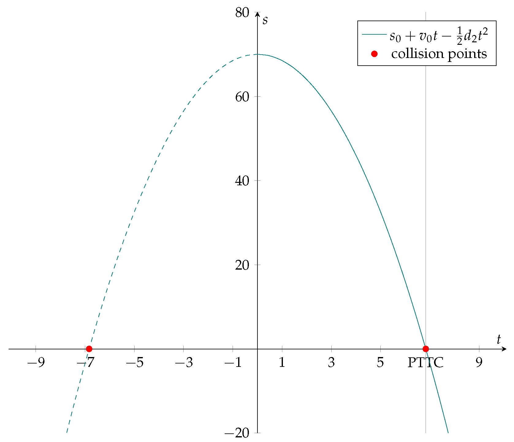
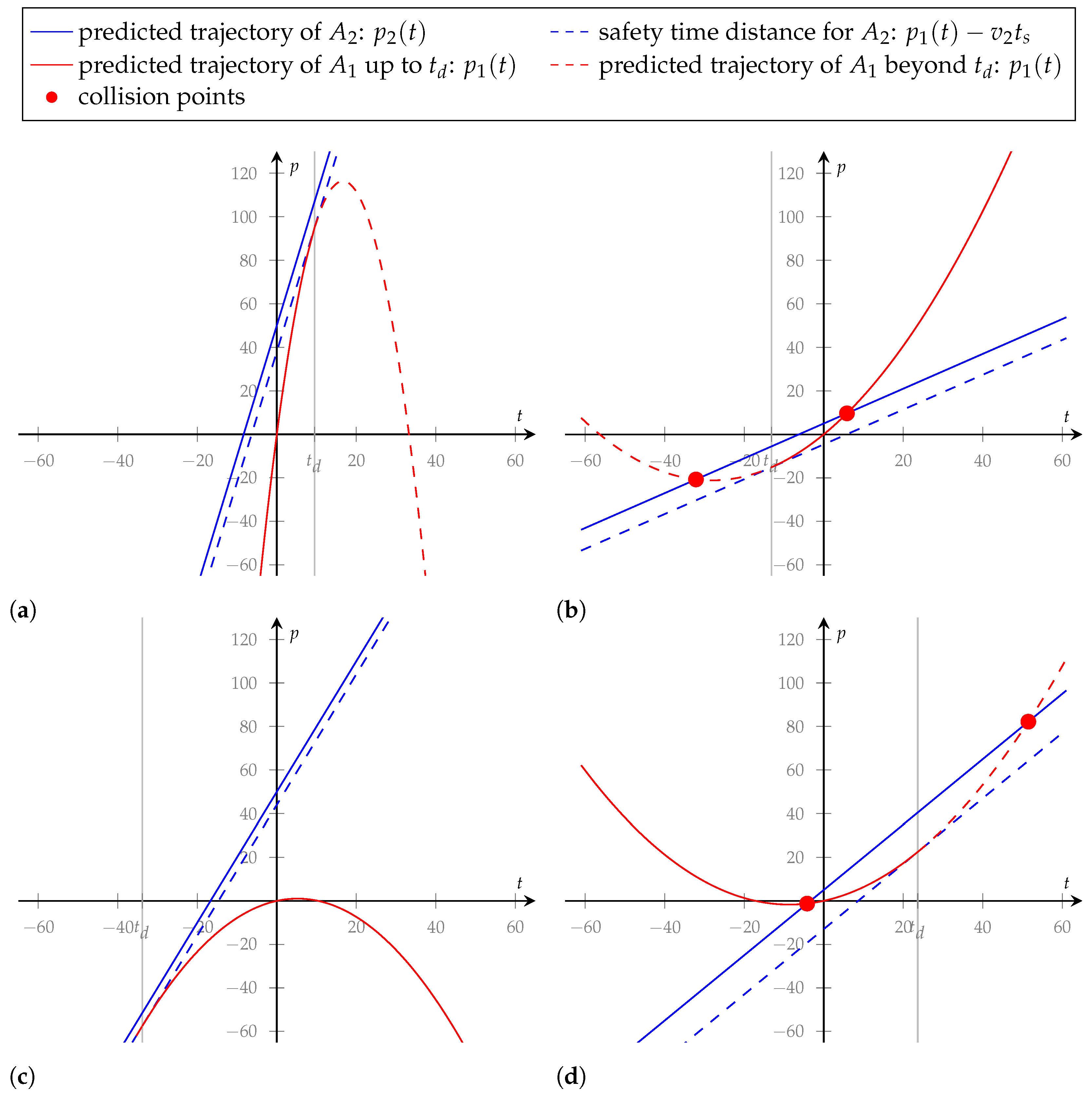
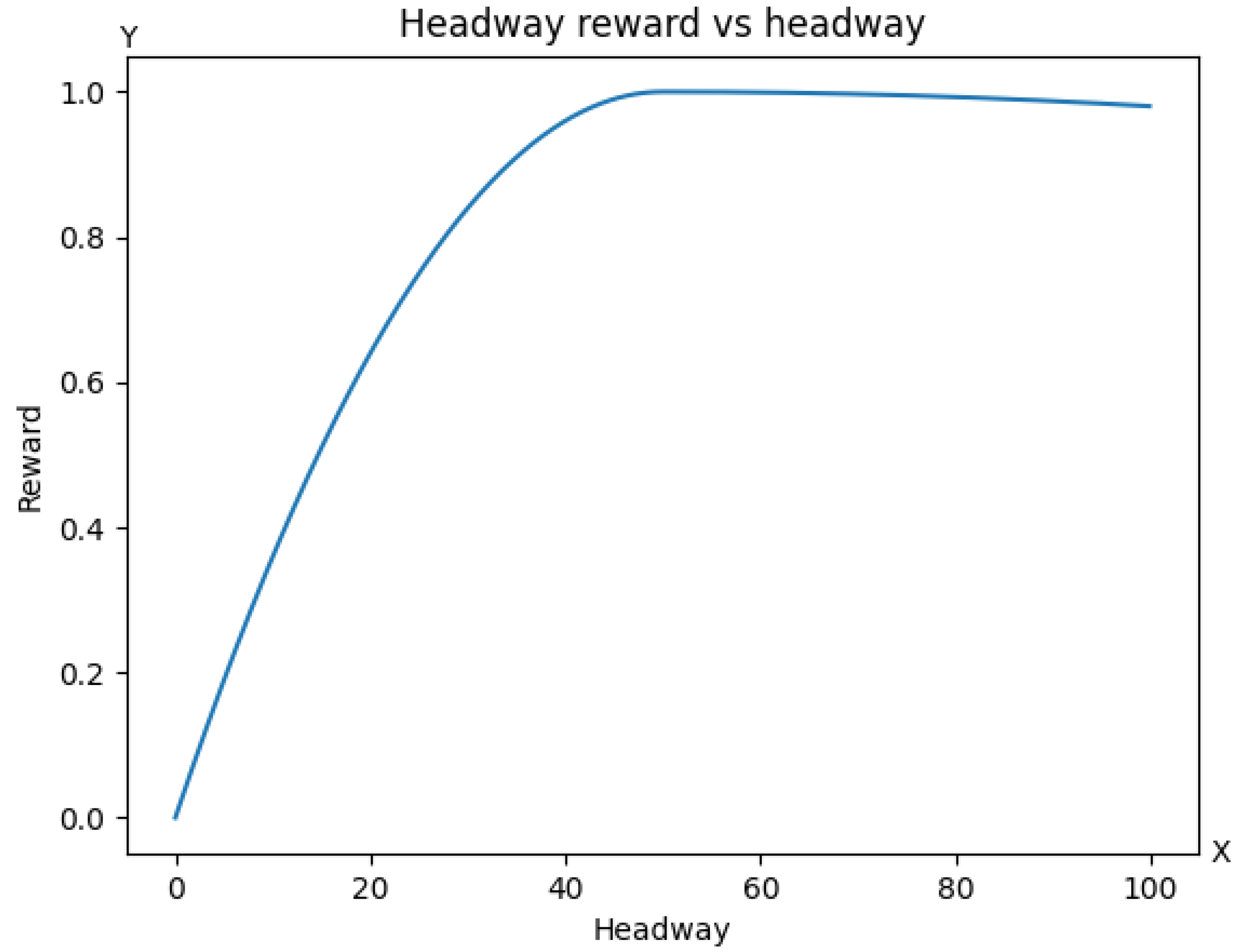
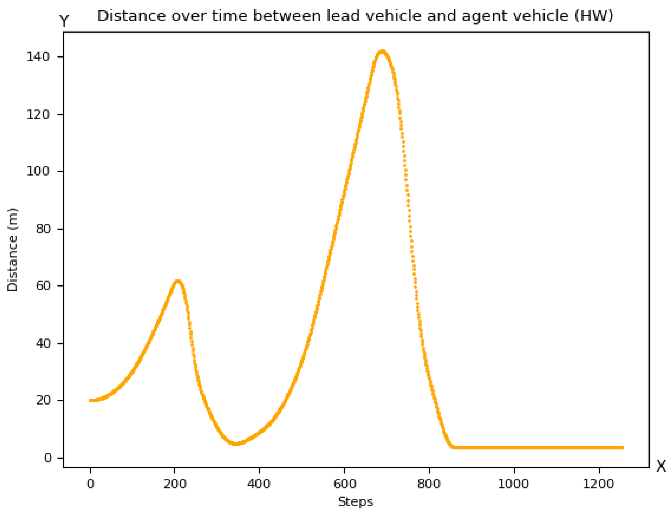
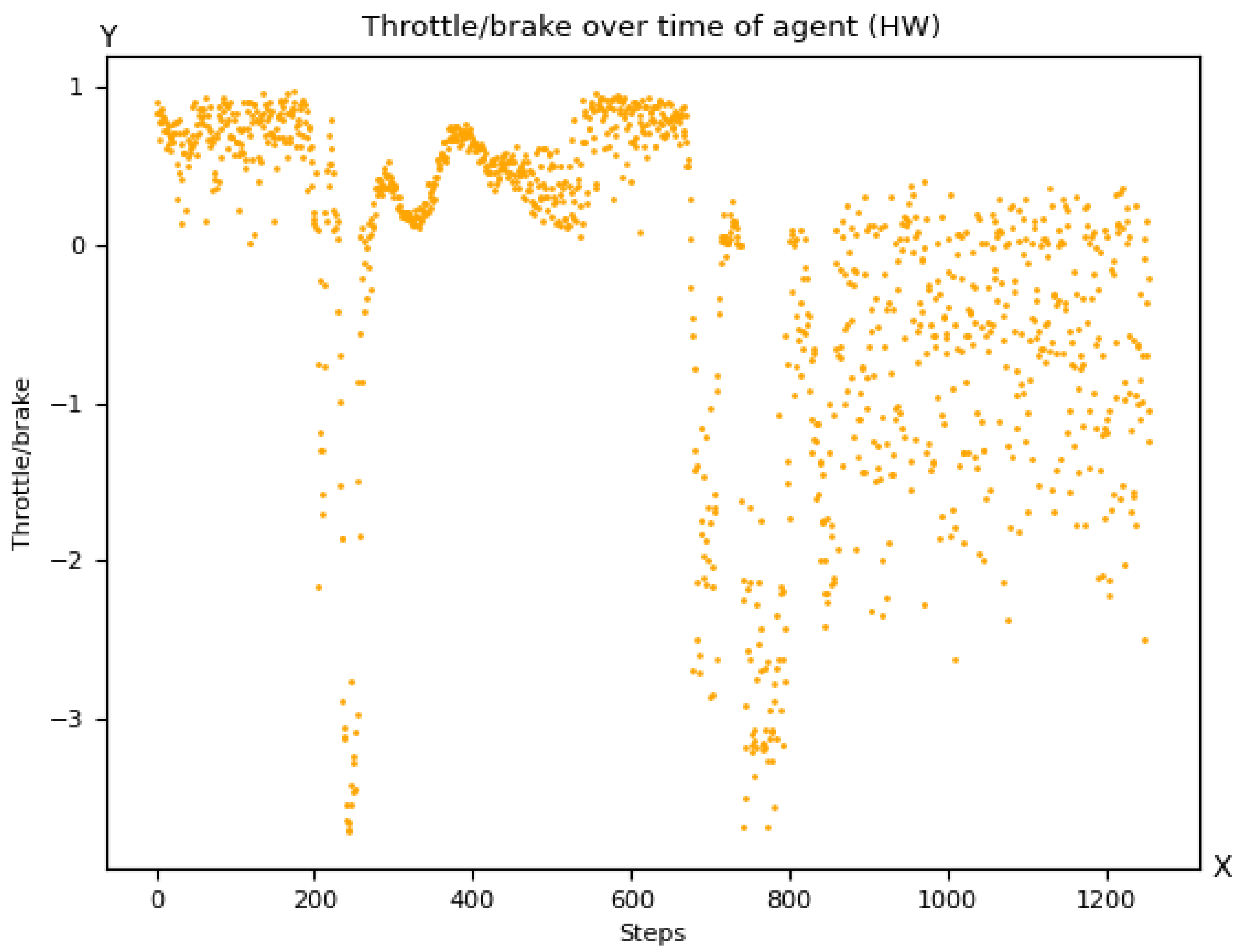
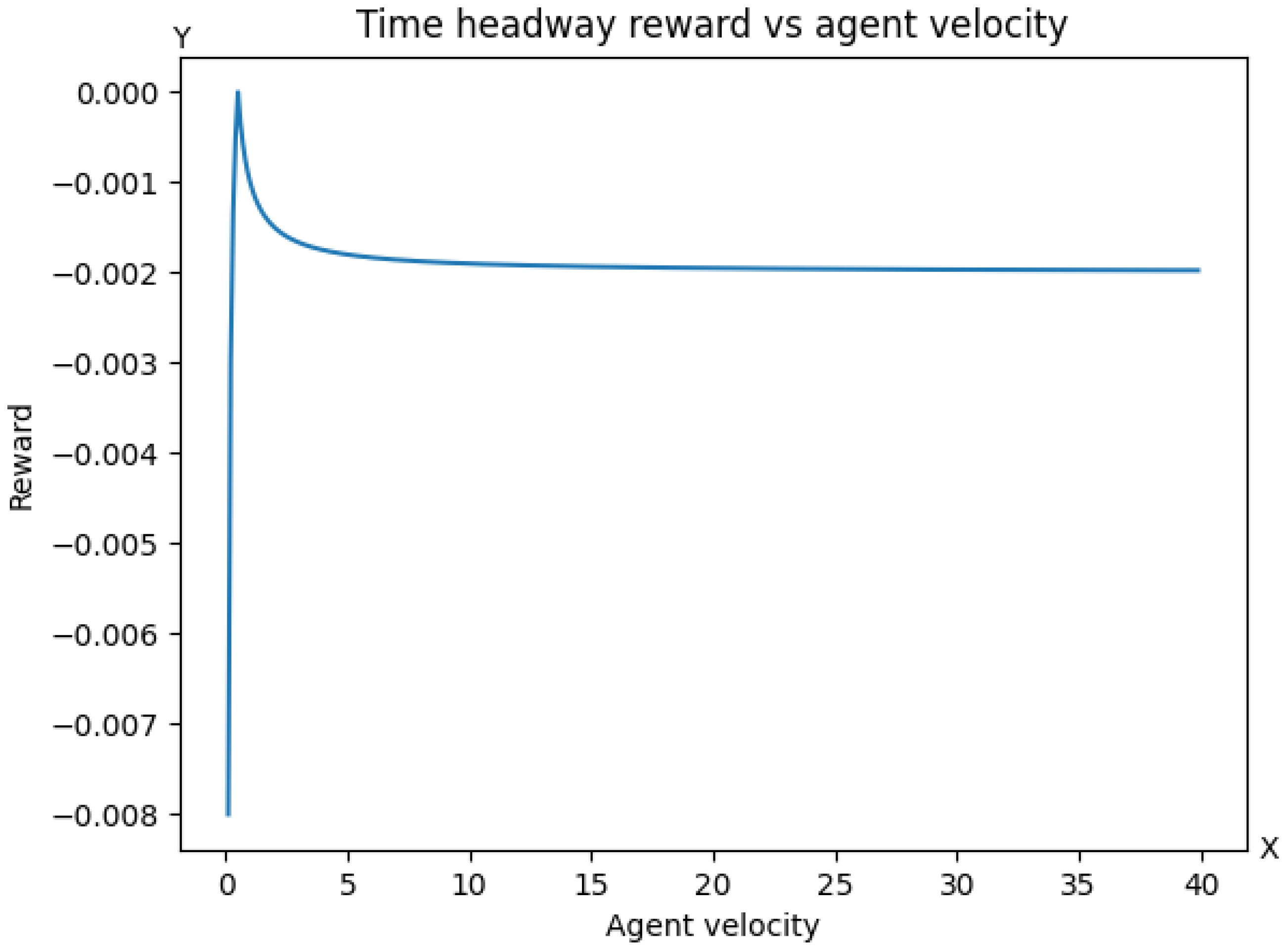
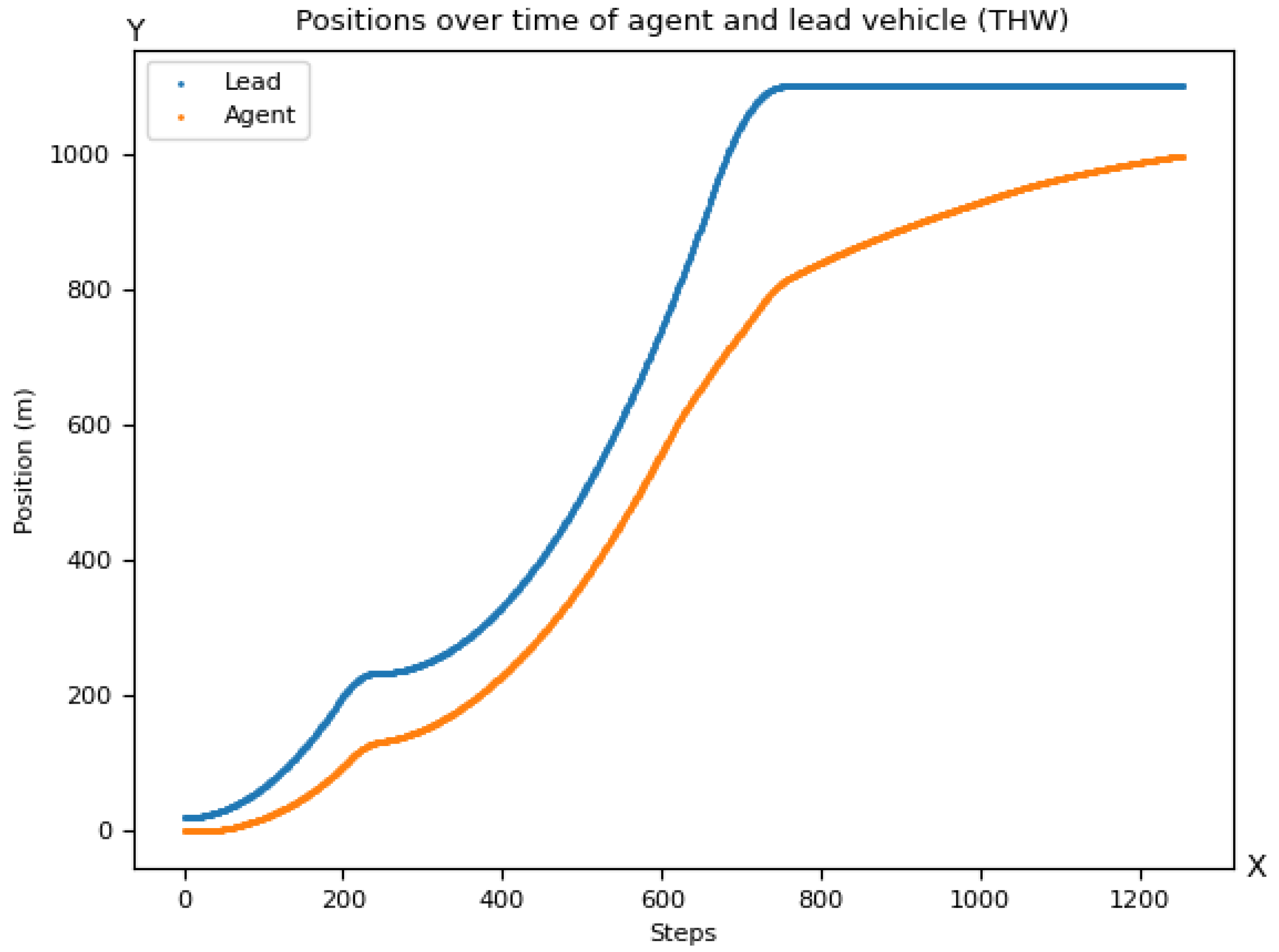
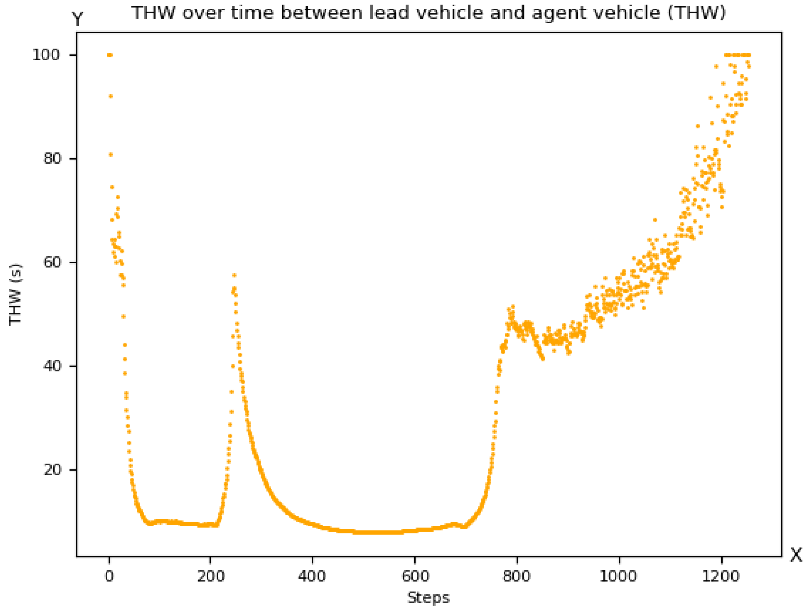
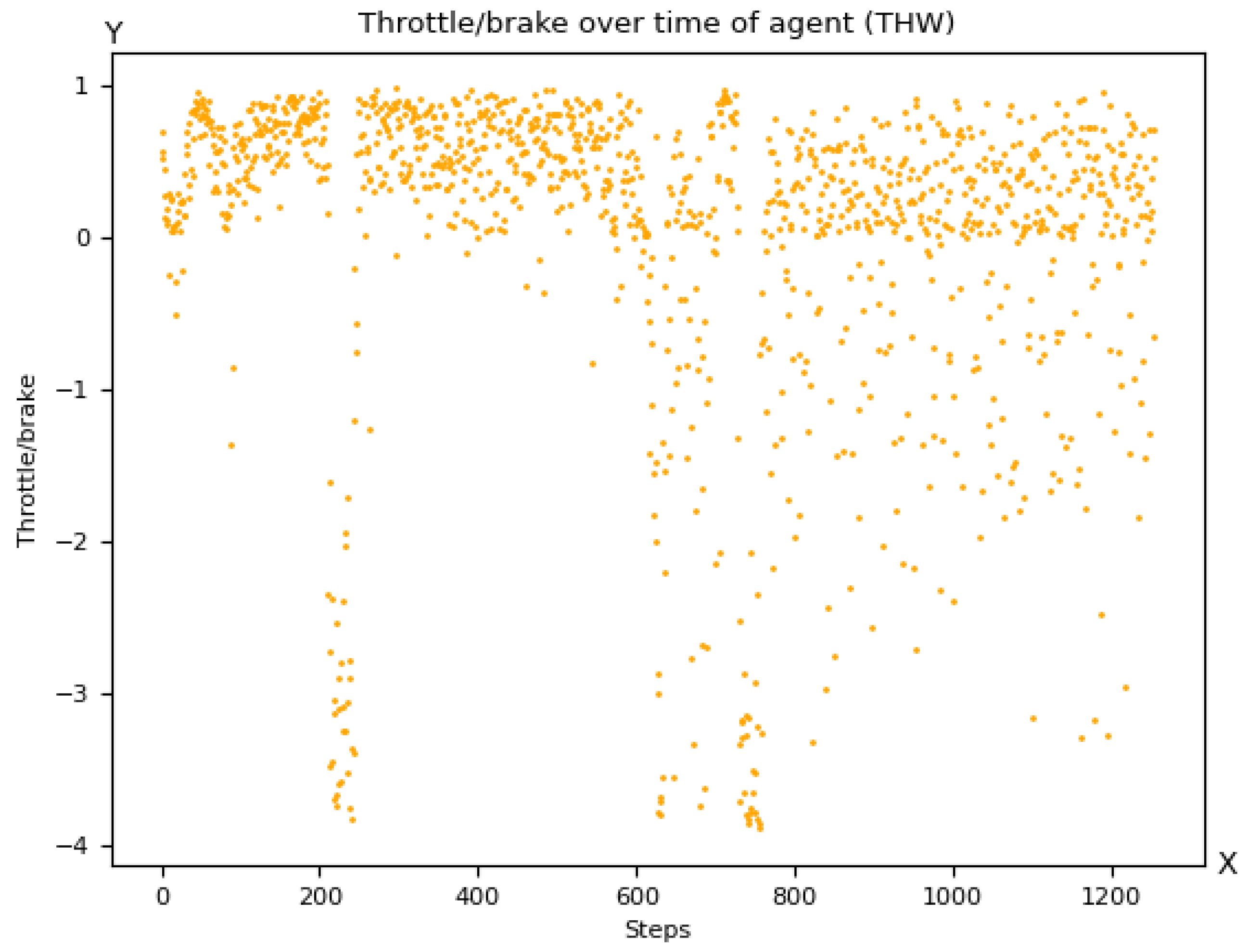
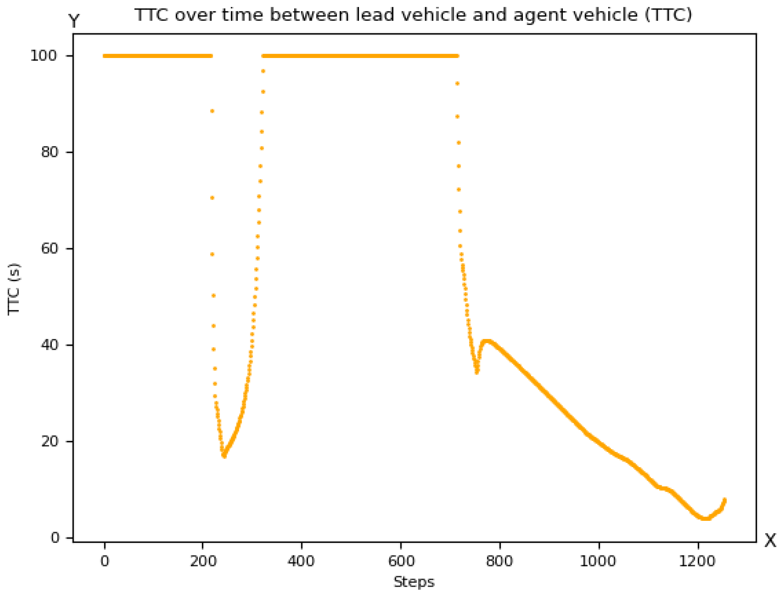
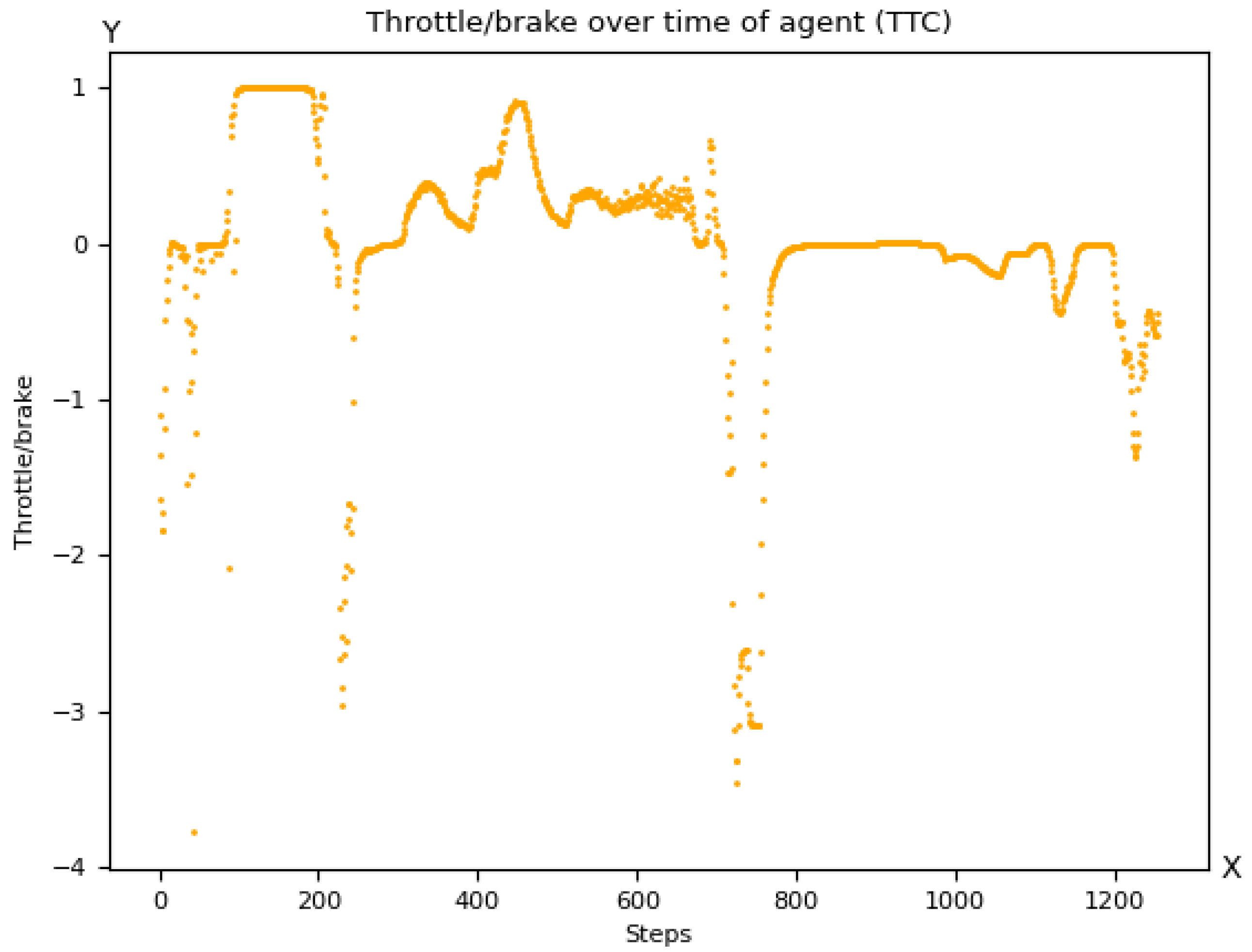
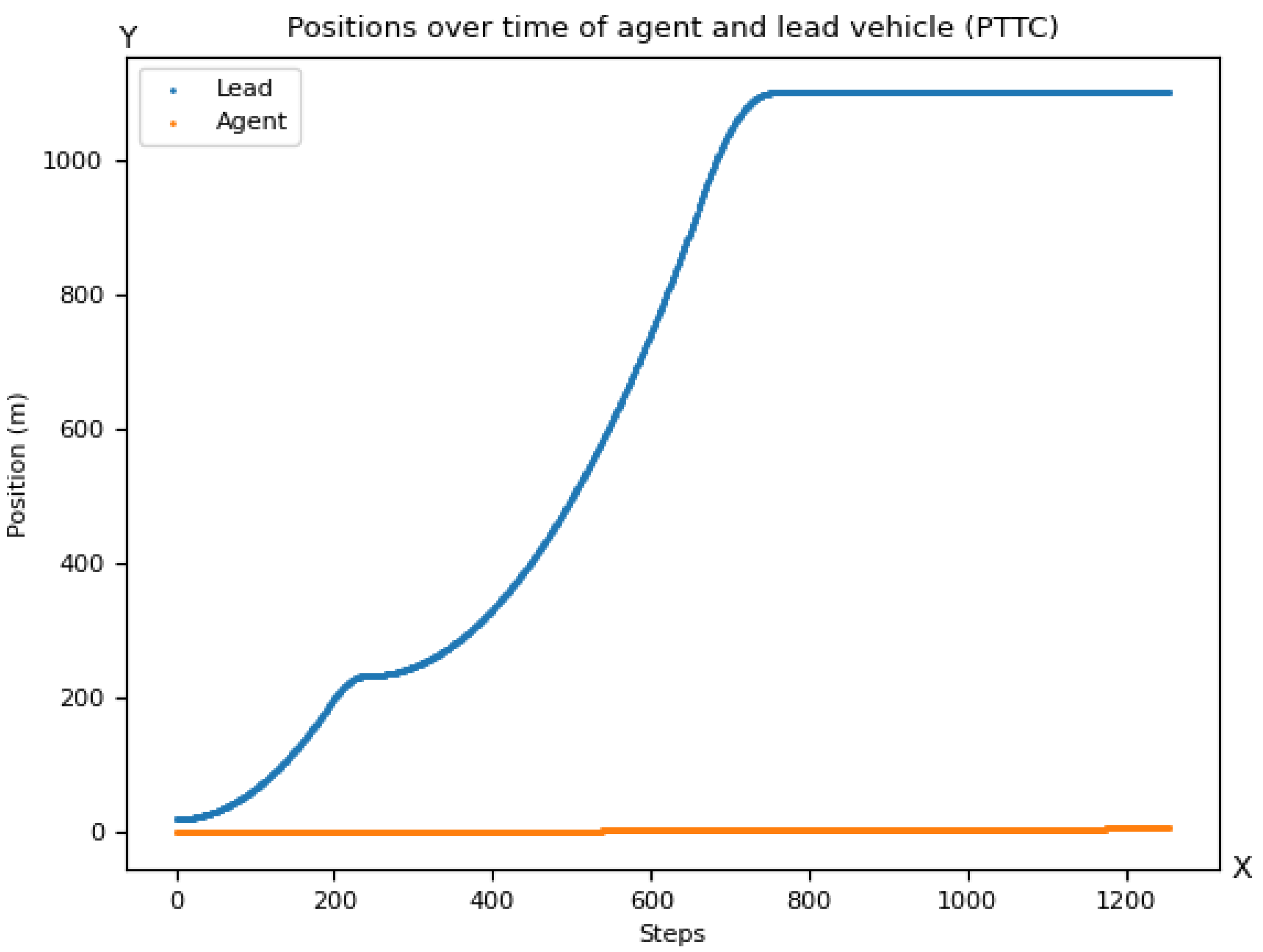
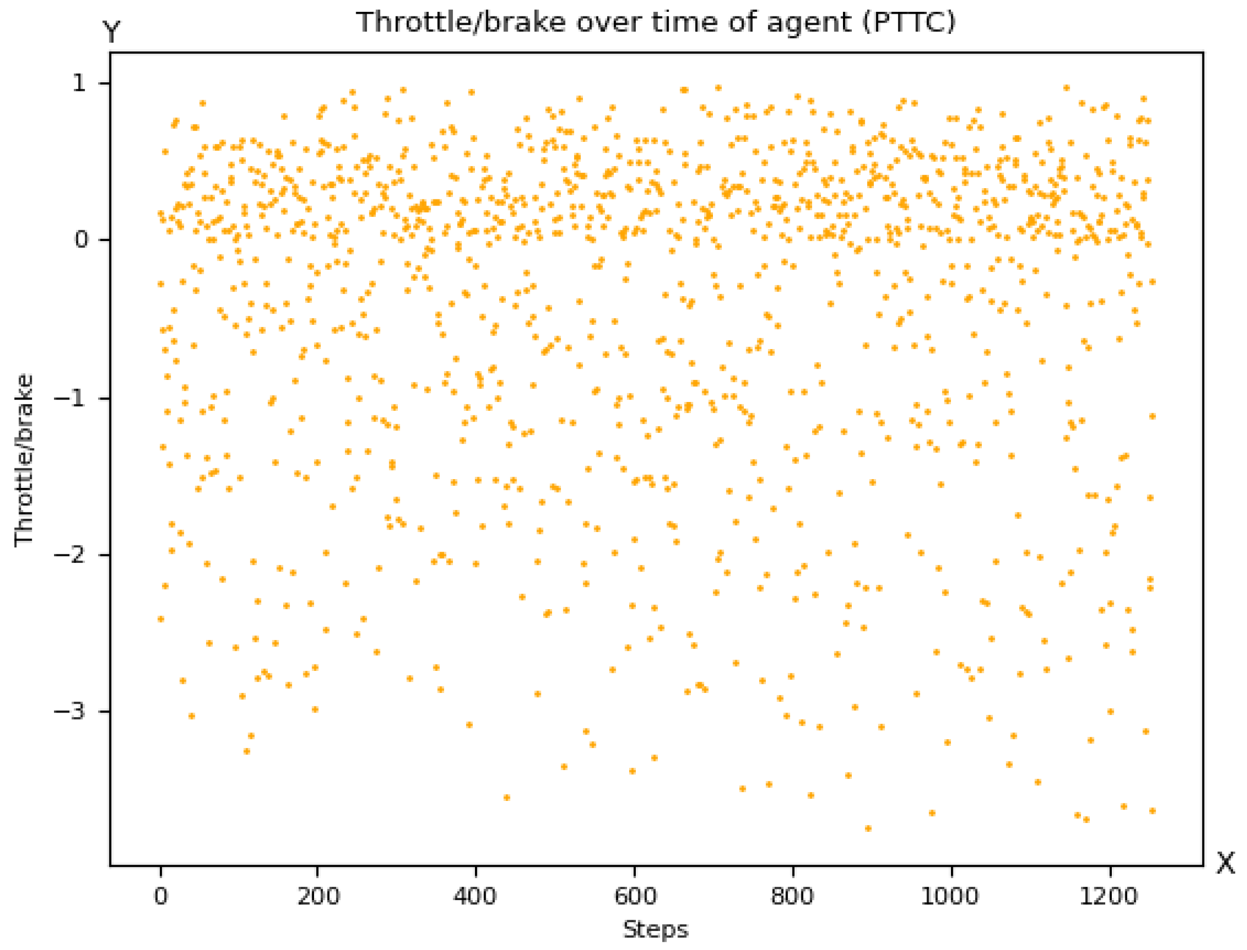
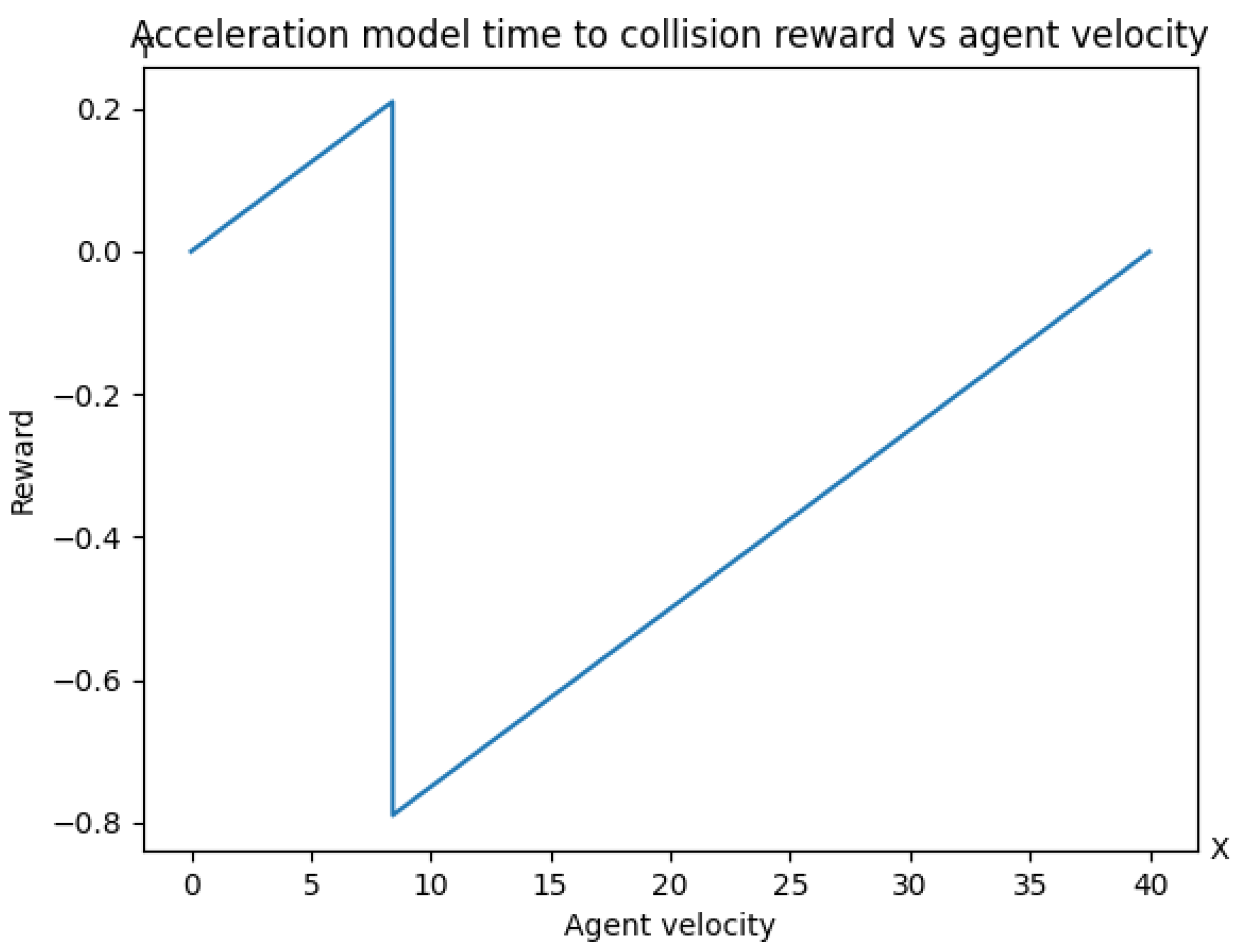
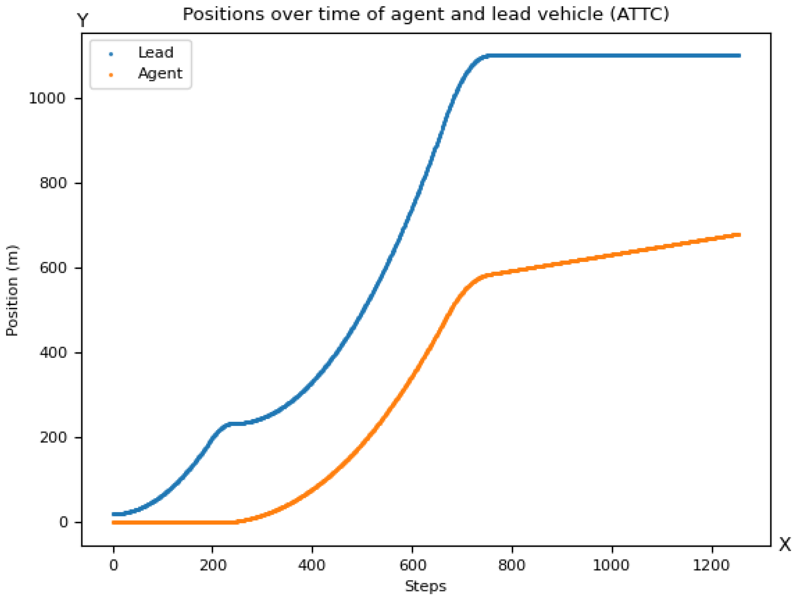
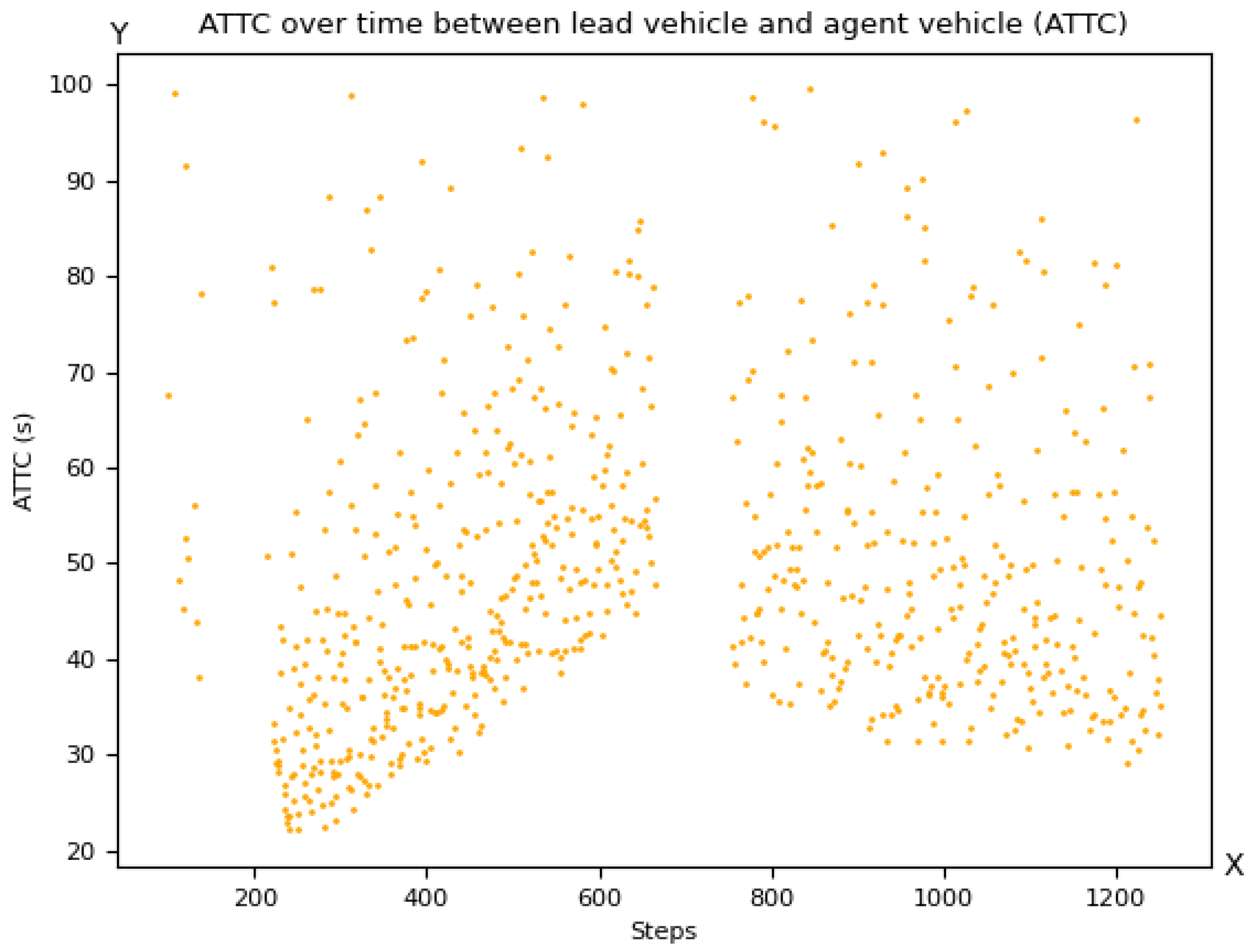
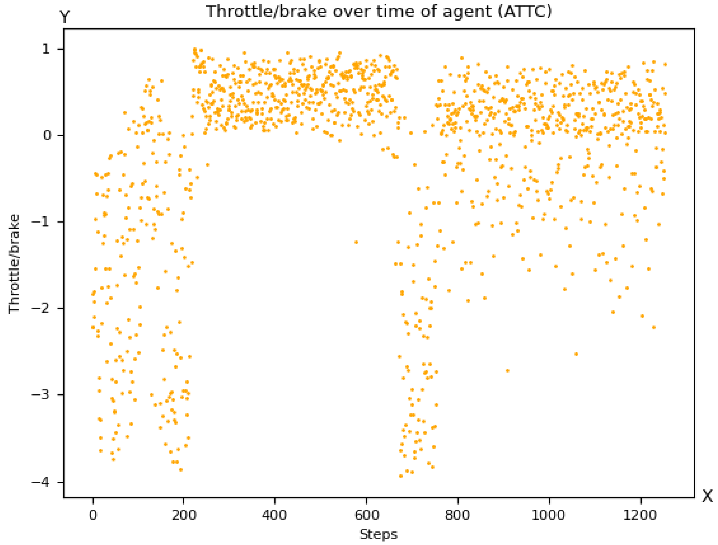
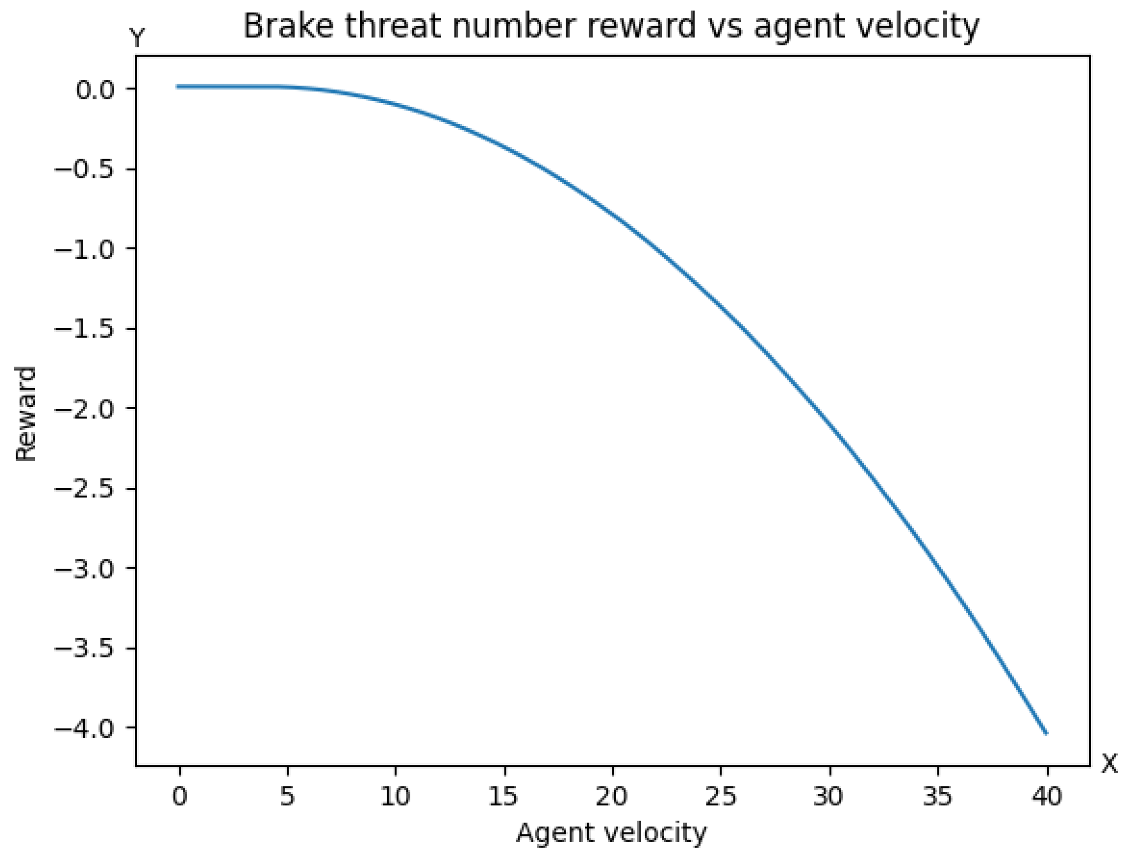
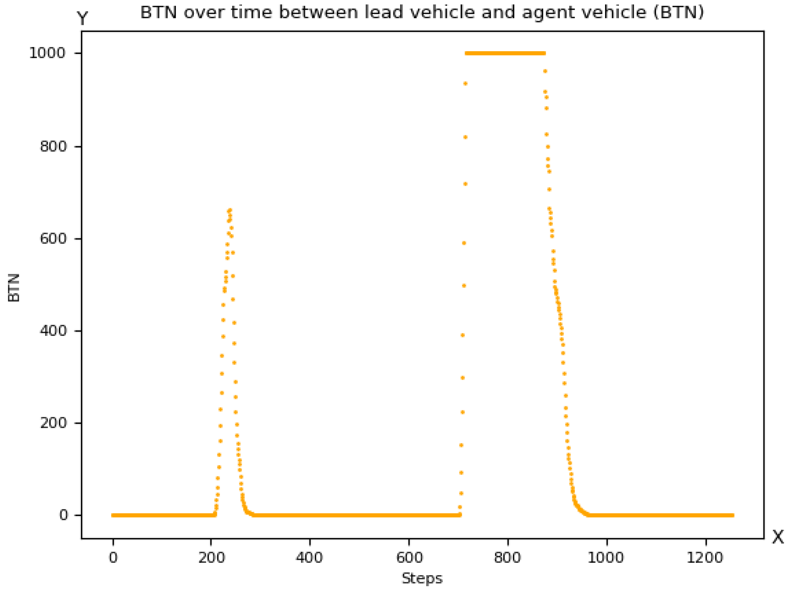
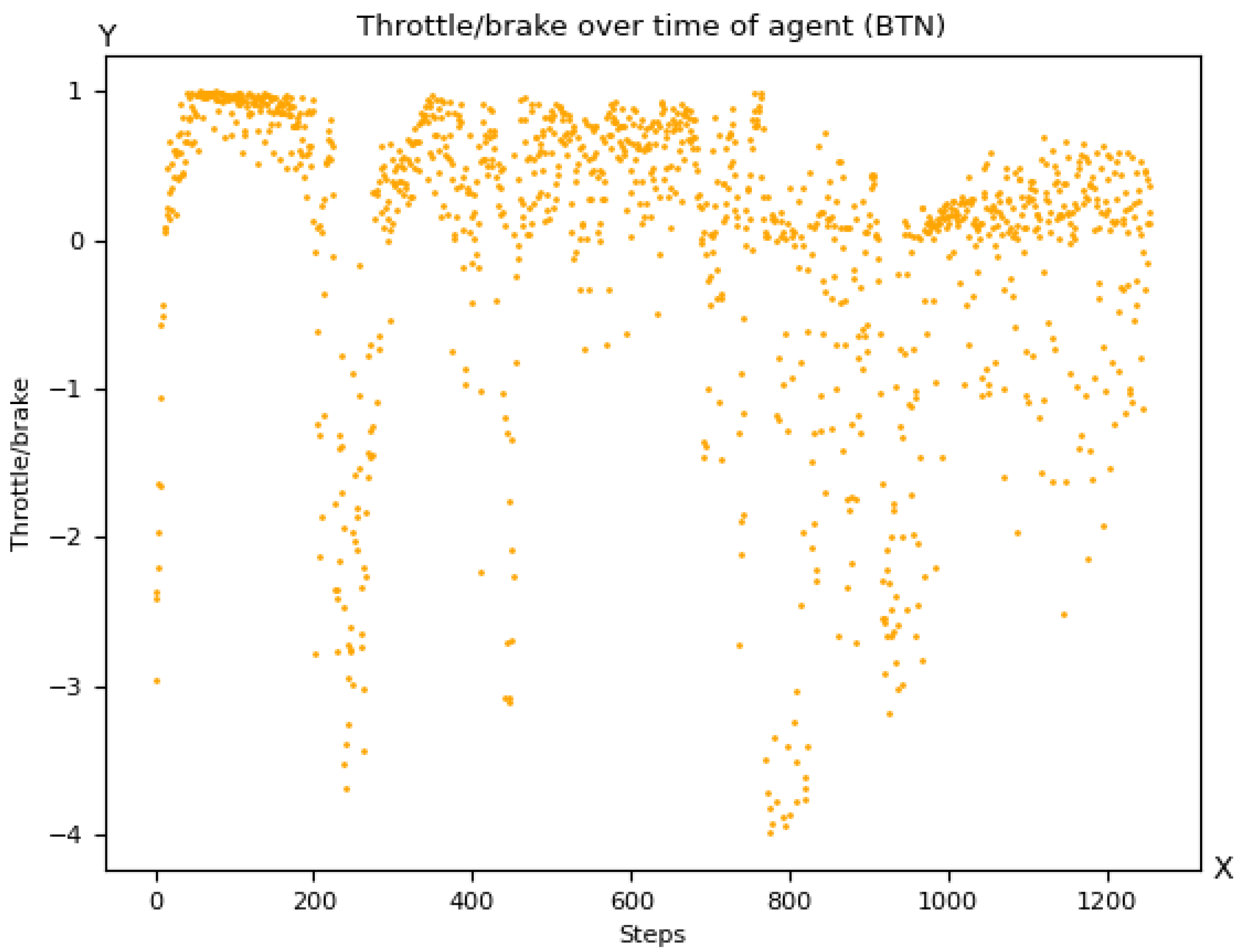
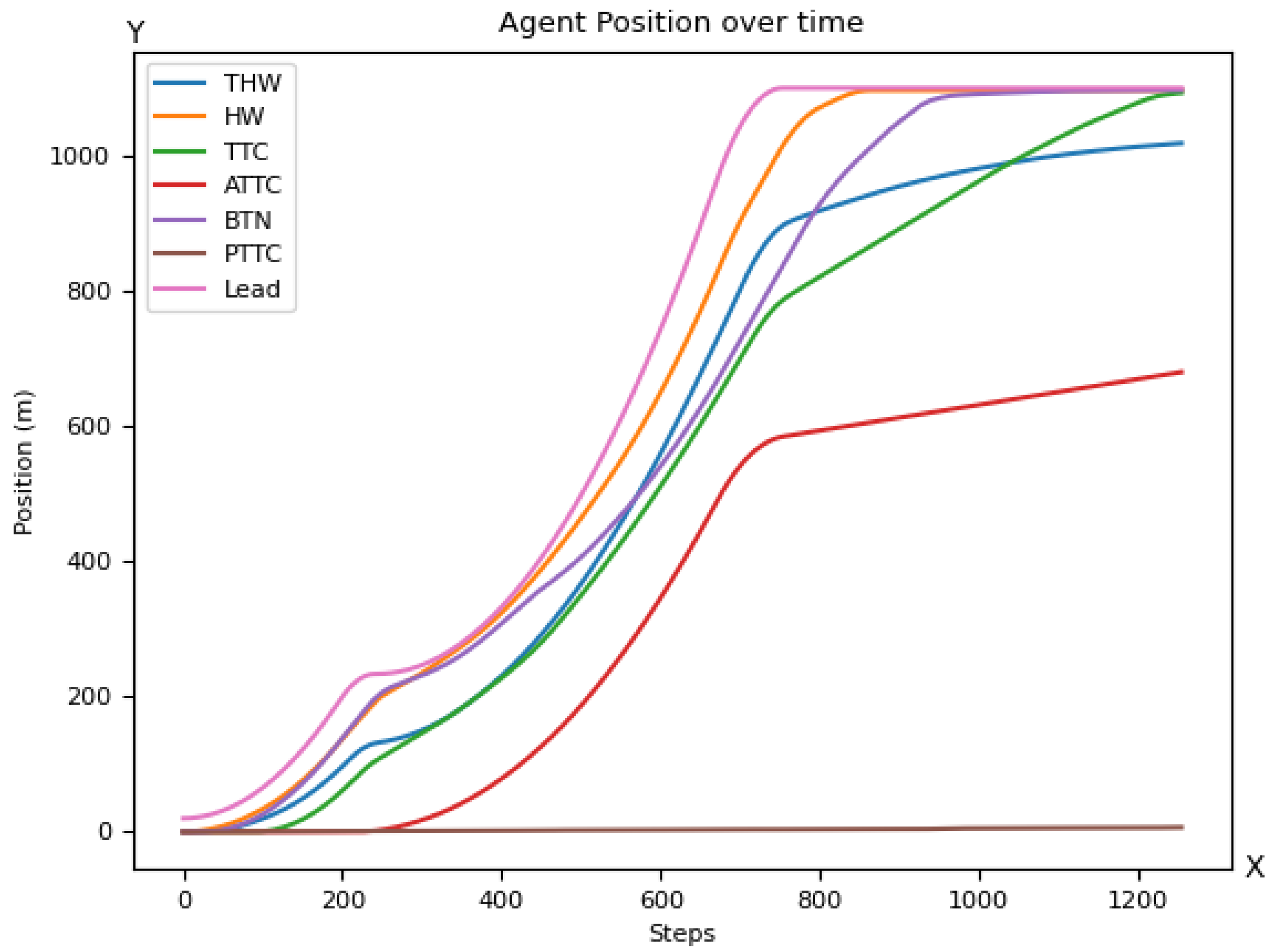
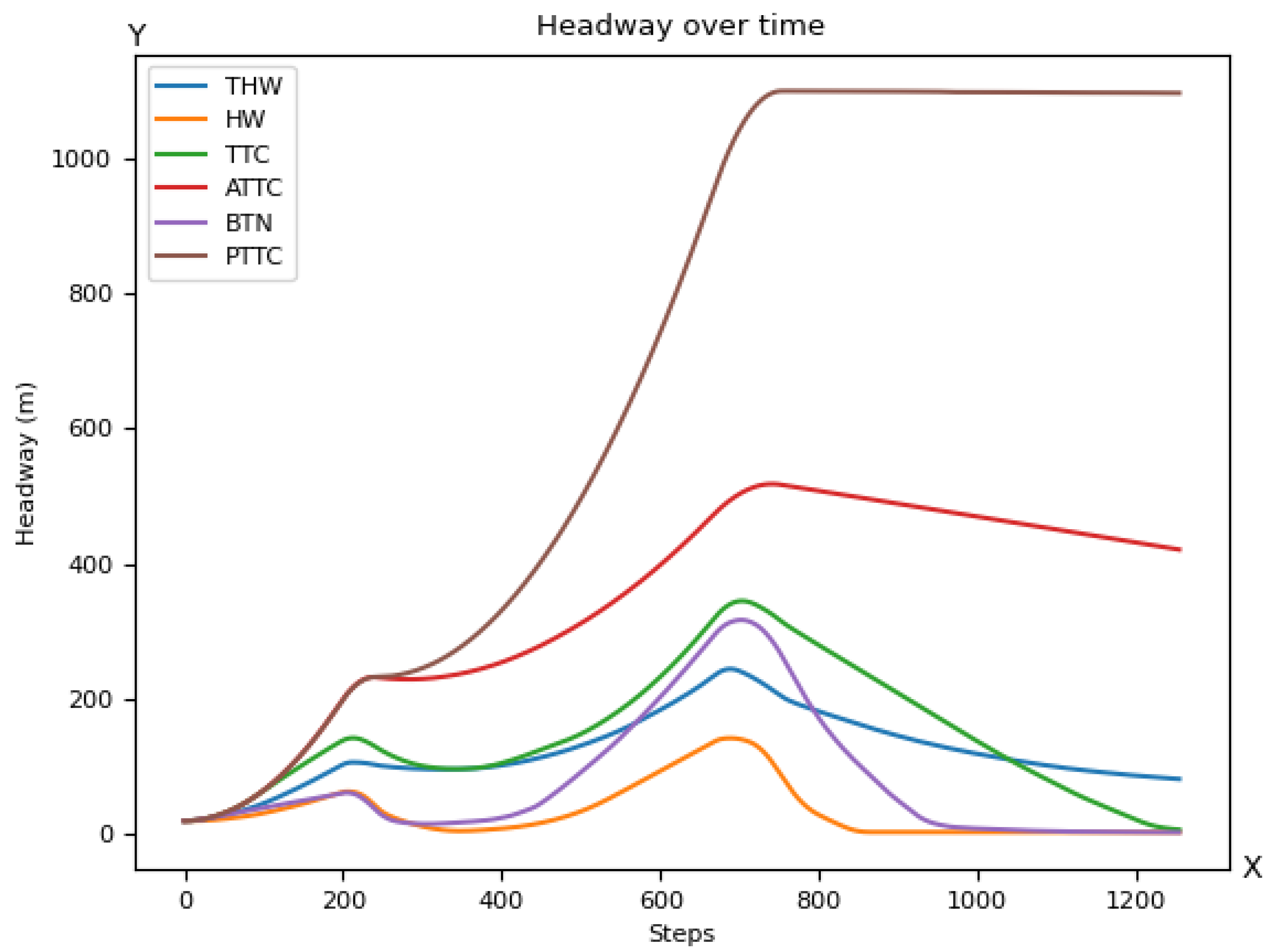
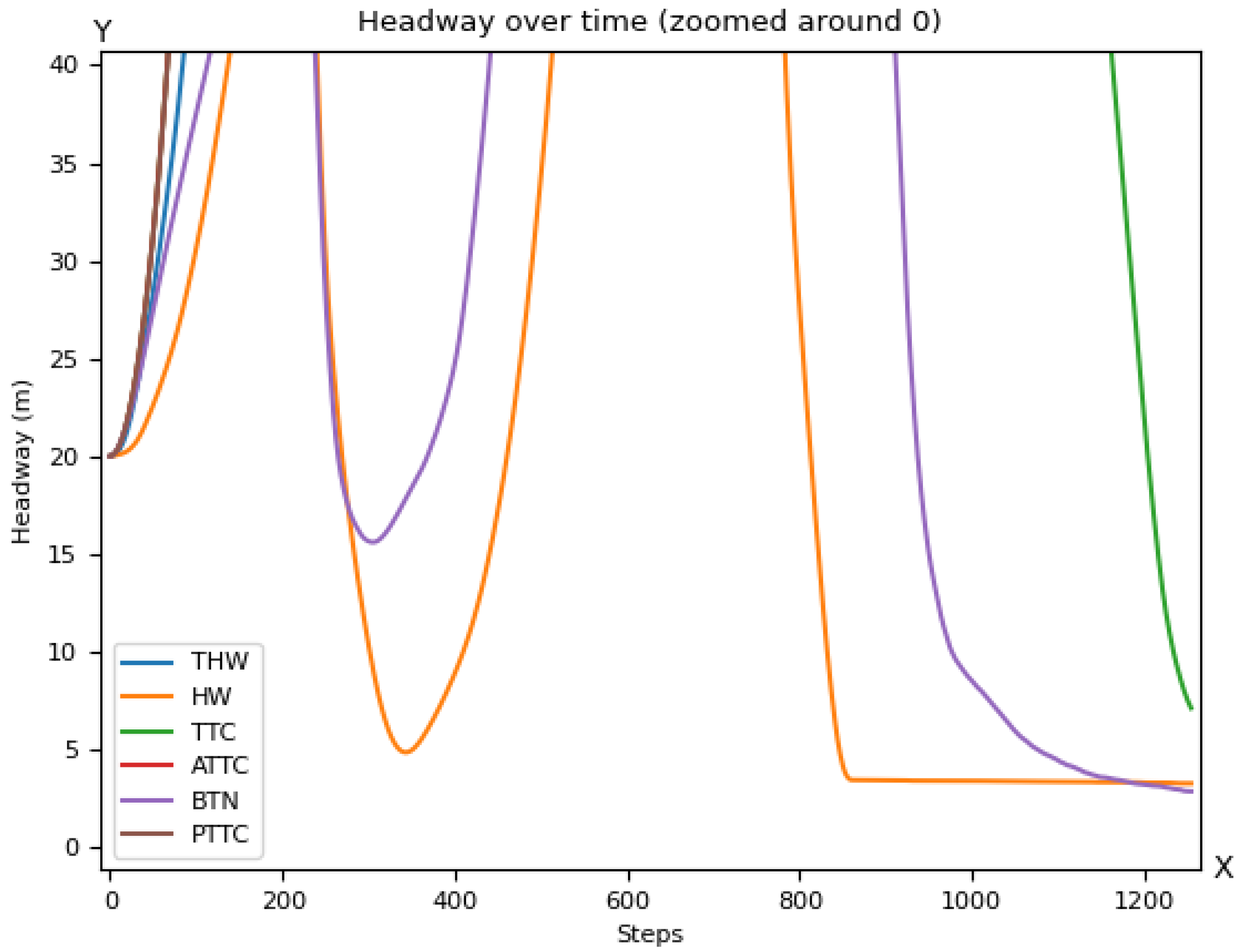
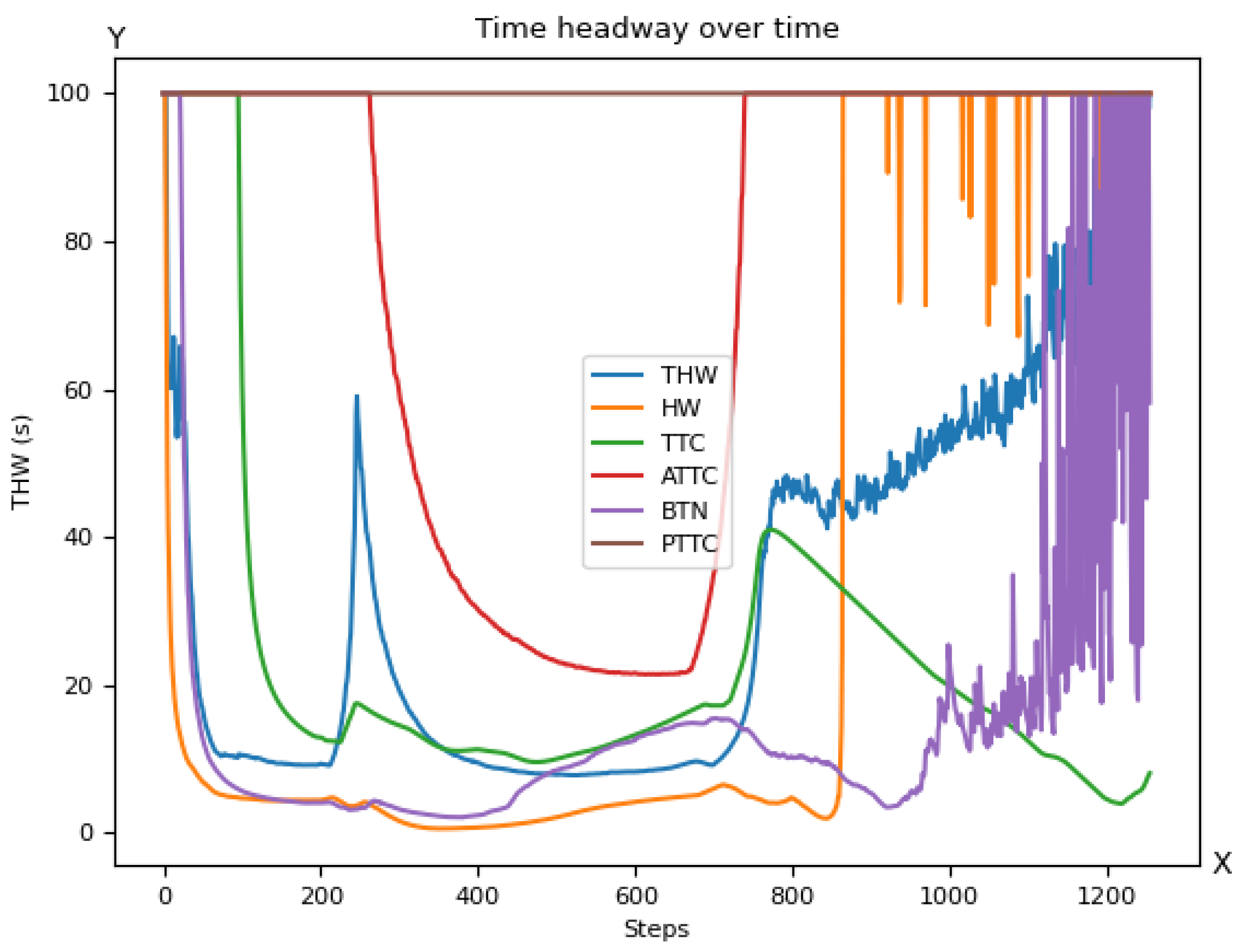
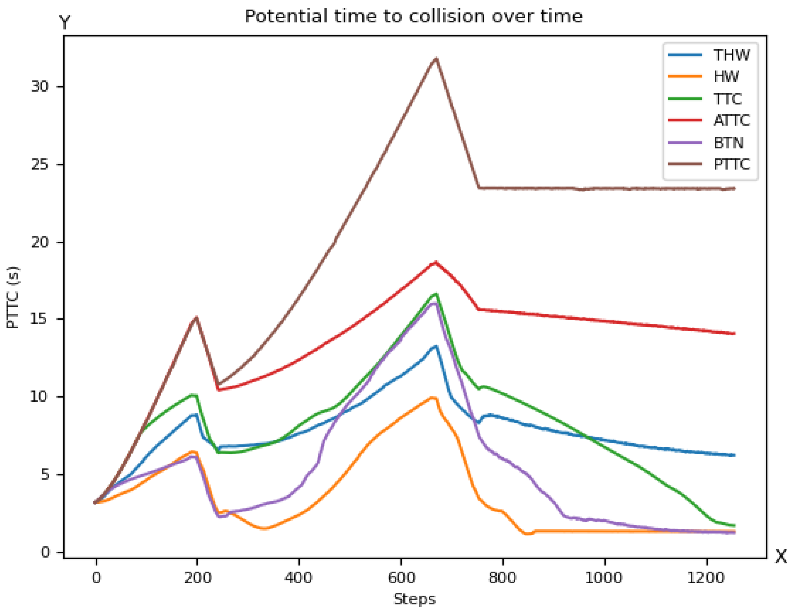
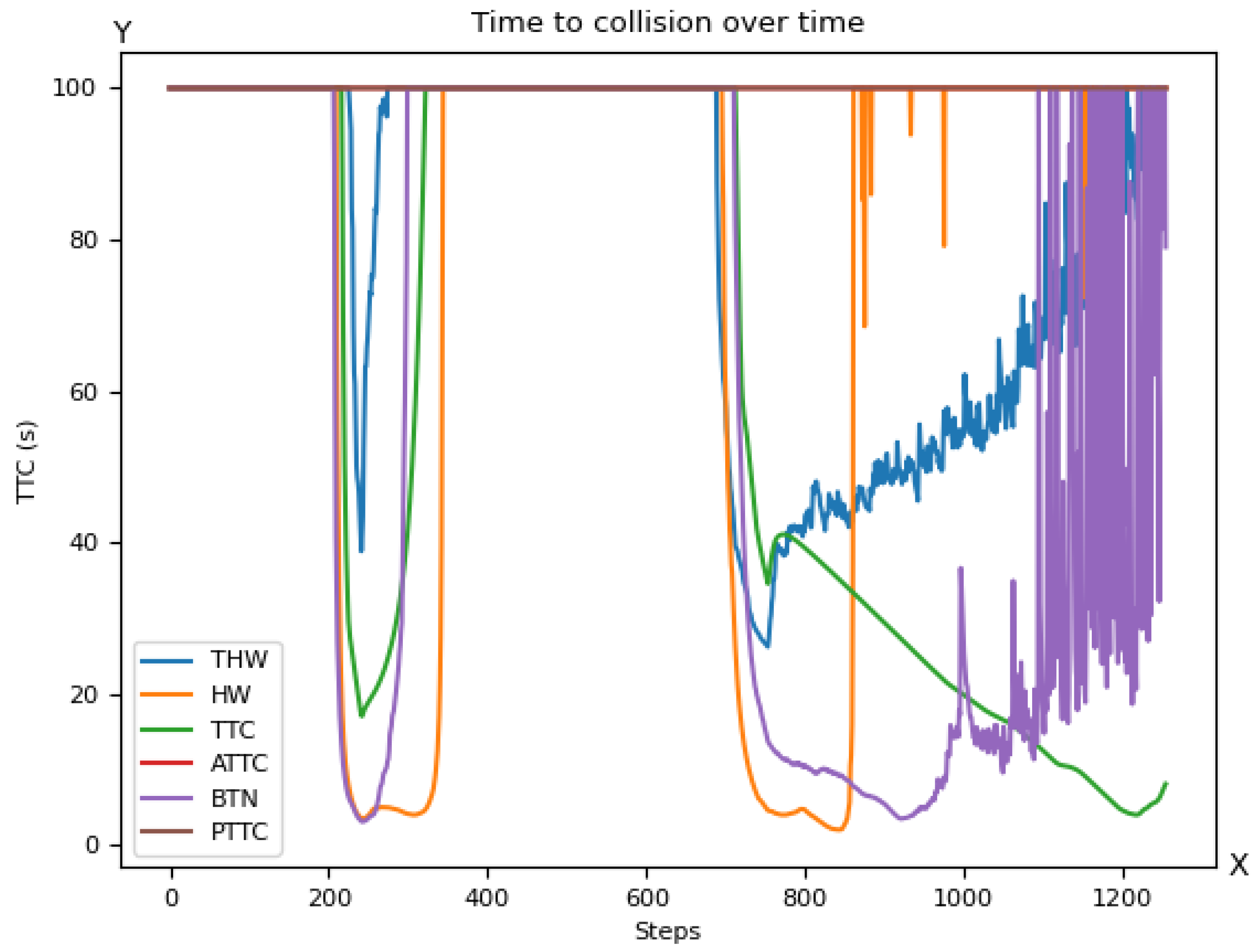
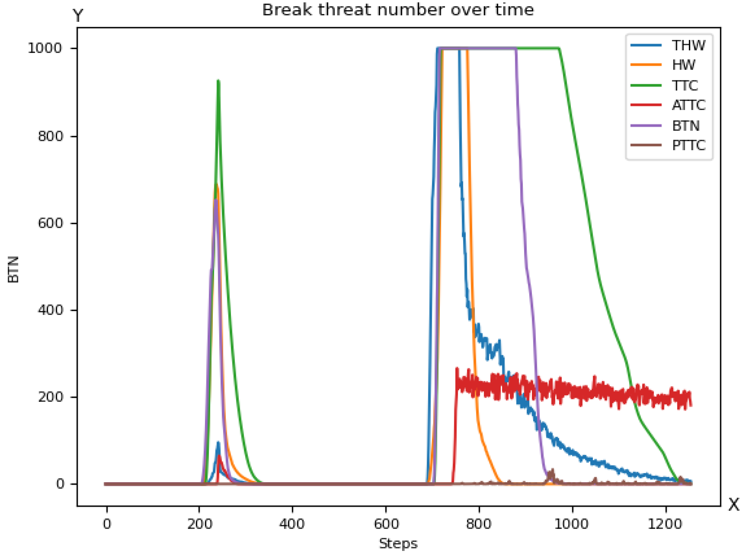