Combining Numerical Simulation and Deep Learning for Landslide Displacement Prediction: An Attempt to Expand the Deep Learning Dataset

Abstract

Effective landslide hazard prevention requires accurate landslide prediction models, and the data-driven approaches based on deep learning models are gradually becoming a hot research topic. When training deep learning models, it is always preferable to have a large dataset, while most available landslide monitoring data are limited. For data missing or data sparseness problems, conventional interpolation methods based on mathematical knowledge lack mechanism interpretability. This paper proposes that numerical simulations can be used to expand the deep learning dataset we need. Taking the Jiuxianping landslide in the Three Gorges Reservoir Area (TGRA) as the geological background, a finite element numerical model was established, and the landslide displacement time series data were solved considering the boundary conditions of reservoir water level change and precipitation. Next, based on three metrics: Euclidean distance, cosine similarity, and dynamic time warping (DTW) distance, the time series similarity between the displacement data obtained from simulation and data obtained from actual monitoring were verified. Finally, the combined deep learning model was built to predict the displacement of the Jiuxianping landslide. The model was trained on both the simulated and monitored datasets and tested by the last 12 monitored data points. Prediction results with the testing set showed that the models trained using the expanded training set from numerical simulations exhibited lower prediction errors, and the errors had a more concentrated distribution. The results suggest that this landslide displacement prediction method combining numerical simulation and deep learning can solve the problem of inadequate datasets due to low monitoring frequency, as well as provide an interpretation of the physical mechanism for data vacancy filling.

1. Introduction

Landslides are one of the most devastating geological hazards in the world, causing significant loss of life and severe property damage [1,2,3,4,5,6]. Complex geological conditions and variable environmental factors combined with human activity-induced disturbances often lead to the sudden occurrence of landslides: for example, the rock slide disaster in Guinsaugon, Philippines in 2006 [7], the Oso landslide disaster in Oso, Washington, USA in 2014 [8], the landslide of the construction waste landfill in Guangming New District, Shenzhen, China in 2015 [9]. China has been one of the countries with the highest frequency of geological disasters in the world. According to relevant statistics from the National Bureau of Statistics (http://www.stats.gov.cn/tjsj/ndsj/, 6 April 2022), more than 100,000 geological disasters occurred in China in the last decade (from 2011 to 2020), of which landslides accounted for more than 70%.

As the evolution of landslides is complex, nonlinear and uncertain, early warning of landslides is an important approach to disaster risk reduction, and the accurate prediction of landslide hazards is a challenging topic as well. The prediction methods for landslides proposed by scholars in past studies can be mainly classified into mechanism- and model-based methods and data-driven methods [10]. The Japanese scholar Saito proposed the method of slope damage time prediction based on creep theory at an early stage [11,12]. Further researches were conducted to predict the timing of rock falls and rock slides based on long-term deformation monitoring [13,14]. In addition, there were proposed methods based on inverse velocity [15], displacement gradient [16], and landslide triggers [17]. These mechanism- and model-based methods can provide explanations in terms of landslide mechanisms, but can be complex, time-consuming, and not very generalizable [18].

Recent studies have shown that data-driven methods can be applied to landslide displacement prediction. The data-driven methods include various machine learning and deep learning models and their respective improvements, such as artificial neural network [19], support vector machine (SVM) [20], extreme learning machine (ELM) [21], long short-term memory network (LSTM) [22], graph convolutional network (GCN) [23], and more. Guo et al. [24] proposed a BP neural network based on wavelet analysis and the gray wolf optimization algorithm, which was successfully applied to the displacement prediction of the Outang landslides. SVM models are commonly used in landslide susceptibility mapping [25], but some improved SVM models have also shown good results in landslide displacement prediction [26,27]. Wang et al. [28] proposed a method for intelligent interval prediction of landslide displacements using a double exponential smoothing method and PSO-ELM model, considering the uncertainty of landslide systems. Deep learning models have been gradually applied to the study of landslide displacement prediction in recent years, mainly including various variants of recurrent neural networks and convolutional neural networks. Xu et al. [29] used empirical mode decomposition method to decompose the Baijiabao landslide displacement into trend component and periodic component, and applied LSTM to the prediction of periodic terms. Zhang et al. [30] successfully predicted the deformation characteristics by capturing the displacement history information of the Jiuxianping landslide with a gated recurrent unit (GRU). Jiang et al. [31] presented a GC-GRU-N model combining GCN and GRU, which exhibited stronger landslide displacement prediction capability than other models.

These data-driven models are widely used as they can predict landslide displacements without too much prior knowledge. However, as various deep learning models have more and more layers and increasingly complex structures, the interpretability of the models is becoming worse. Moreover, the big data that matches the deep models are rarely seen in the field of geohazards. Most landslide displacement predictions use only a few dozen to a few hundred data points [32,33,34], including numerous landslide prediction studies in the Three Gorges Reservoir area (TGRA) in China [10,21,22,32,33,35]. It is obvious that this situation cannot meet the requirements of “big” data and “deep” learning [36]. At this time, attention can be focused on numerical simulation approaches, which can uncover the laws behind physical phenomena and provide the training data required by deep learning models [37]. Again, taking the TGRA landslides as examples, some studies based on numerical simulation fully considered the physical and mechanical properties of landslides, combined with environmental triggers, and explored the landslide deformation mechanism in this area, and the results were in good accordance with the actual monitoring data [38,39,40]. In view of the fact that numerical simulations can explain the internal physical mechanism of landslides, it is worth considering the use of numerical simulation methods to obtain the data sets we need.

In this paper, we propose a landslide displacement prediction method based on the combination of numerical simulation and deep learning, using the Jiuxianping landslide of TGRA as the engineering geological background. Figure 1 presents the flowchart of the analysis. The finite element numerical model is used to generate the training data of landslide displacement needed for deep learning, and the trained deep learning model using simulated displacement data shows good results on the testing set composed of measured data. The prediction is more accurate compared to the model trained with real measurement data. The results of this study provide a new concept for the study of landslide hazard prediction.

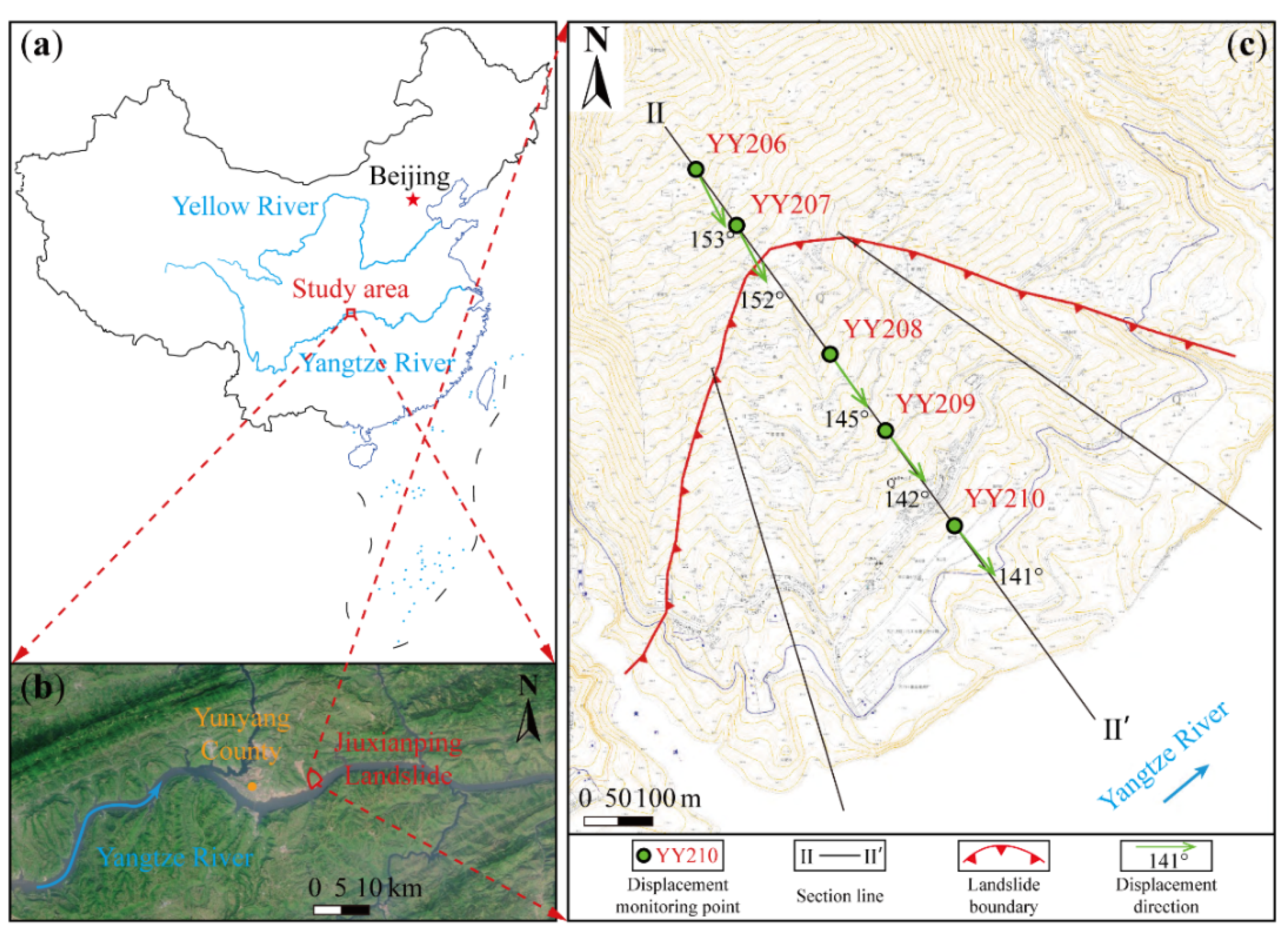
2. Jiuxianping Landslide

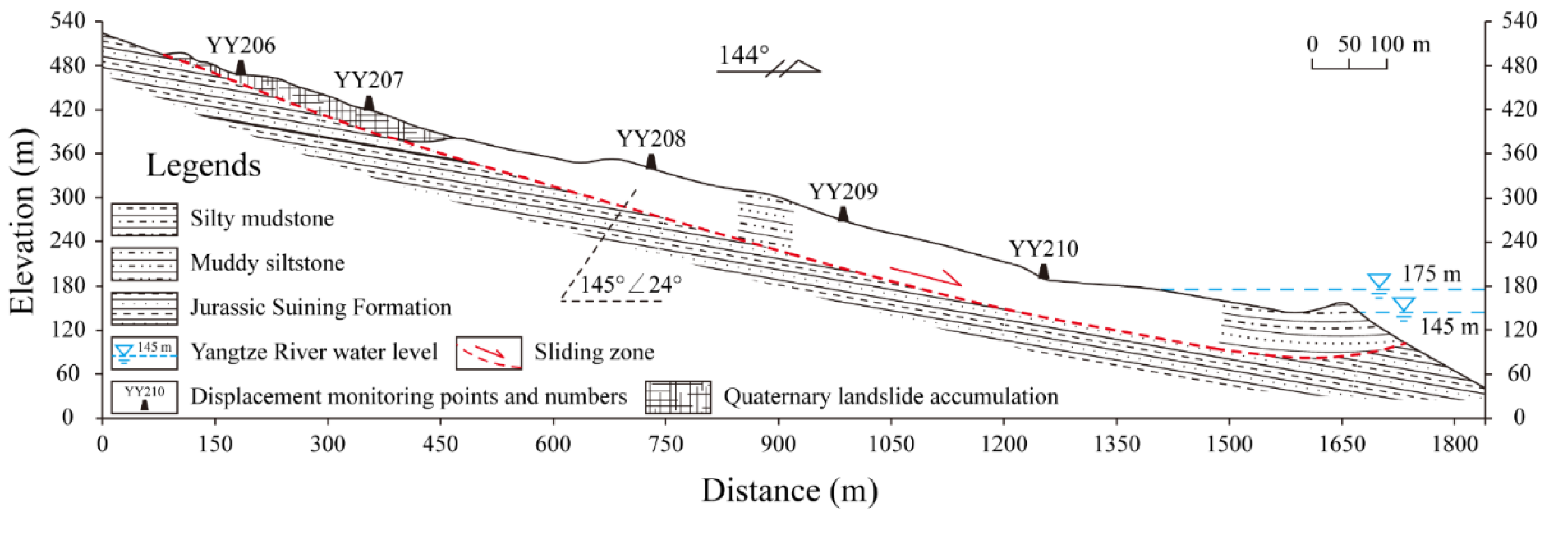
2.1. Regional Background and Geological Structure

The Jiuxianping landslide site is located on the left bank of the Yangtze River in Yunyang County, Chongqing, and about 11.3 km away from Yunyang County (Figure 2). The plane shape of the landslide is nearly circular, the left and right edges are bounded by gullies, and the back edge is bounded by steep bedrock walls. The landslide body has an elevation of about 95 m at the front edge and 385 m at the back edge, a length of about 1200 m, a middle width of about 850 m, an average thickness of about 40 m, an area of about 1.44 km², and a volume of about 5.7 × 107 m³, and it was a large bedding rock landslide with the front edge wading. There are three monitoring sections in the east, middle and west of the landslide. This paper selected the monitoring data and geological data of the II-II′ section in the middle of the landslide for study.

The site of the Jiuxianping landslide is located on the north side of the Huangbaixi syncline, with no fracture structure development. Both the landslide body and bedrock are composed of grayish-white sandstone, purplish-red muddy siltstone and silty mudstone of the Jurassic Suining Formation, and the surface of the landslide is covered with gravel mixed with silty clay. The upper and middle parts of the Jiuxianping landslide have a dip of about 15° to 30°, and the front edge of the landslide has an upward warping. The main sliding direction of the II-II′ section of the Jiuxianping landslide is approximately 144° (Figure 3). The front of the landslide is exposed or partially submerged intermittently by the rise and fall of the reservoir water level, which fluctuates between 145 m and 175 m.

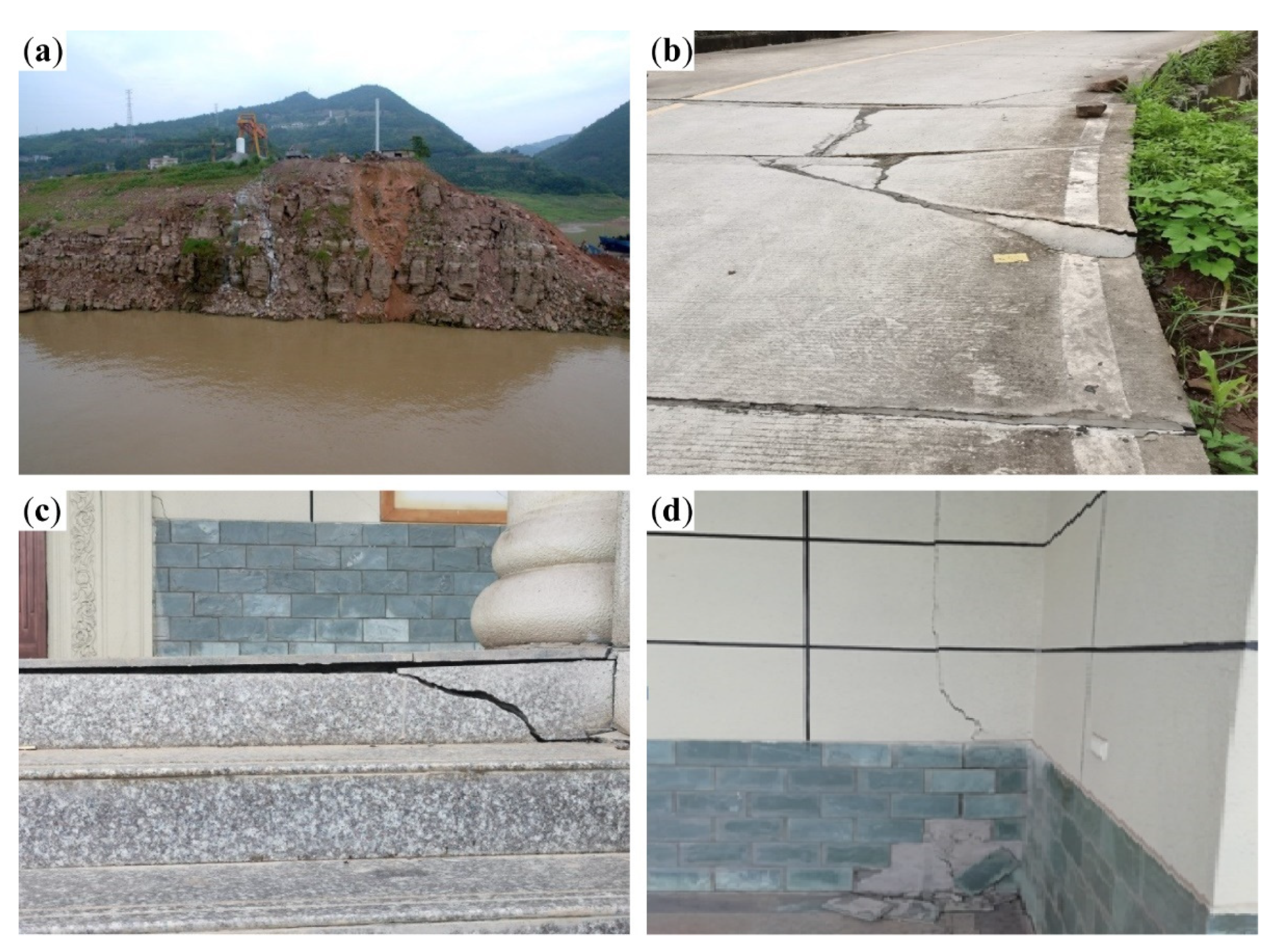
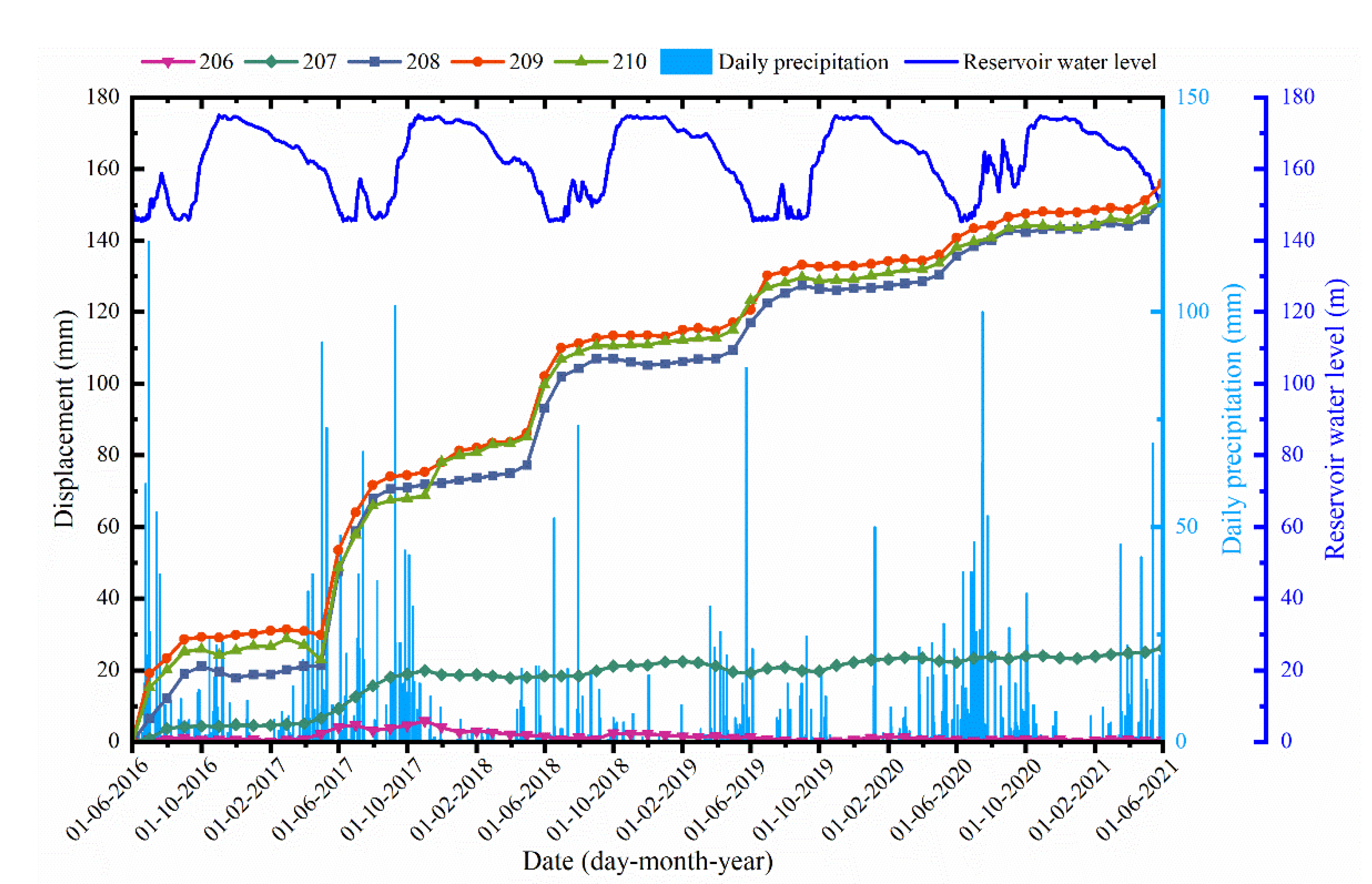
2.2. Monitoring Results

Surface deformation observations of the Jiuxianping landslide began in 2016. Figure 3 illustrates the surface deformation of the landslide at various locations. The front edge of the landslide is reverse deformed by the erosion of the Yangtze River, providing favorable conditions for damage (Figure 4a). Cracks in the mountain road continue to widen and the ground uplifts slightly (Figure 4b). Visible cracks and deformations appear in the walls and steps of the buildings (Figure 4c,d).

As shown in Figure 2 and Figure 3, in order to monitor the deformation of the Jiuxianping landslide in real time, five GNSS displacement monitoring stations, YY206, YY207, YY208, YY209 and YY210, were arranged on the slope surface along the II-II′ section line. Since June 2016, the five monitoring stations have collected displacement data from these points, and the monitoring frequency of the available data is once a month. At the same time, daily reservoir levels as well as precipitation in this region were recorded.

Figure 5 shows the precipitation, reservoir level and accumulative displacement data for the Jiuxianping landslide from June 2016 to June 2021. The displacement curves display that the front and central parts of the Jiuxianping landslide have been in an unstable state for several years, with deformation continuing to increase stepwise. It can be seen from Figure 5 that the landslide deformation is related to the cyclical changes of the reservoir level and rainfall. The three monitoring points closer to the bank (YY208, YY209, YY210) have a sharp increase in displacement between May and July, which coincides with an increase in rainfall and rapid drawdown of the reservoir water level. In contrast, during the months with less rainfall and periods of rising reservoir levels, slow drawdown and smooth running, the slope displacements are virtually unchanged. Such results are consistent with the findings of previous studies on landslides in the Three Gorges reservoir area [41,42,43]. Data from monitoring sites YY206 and YY207, which are far from the riverbank, indicate that the ancient landslide accumulation near the back edge of the landslide is in a more stable state.

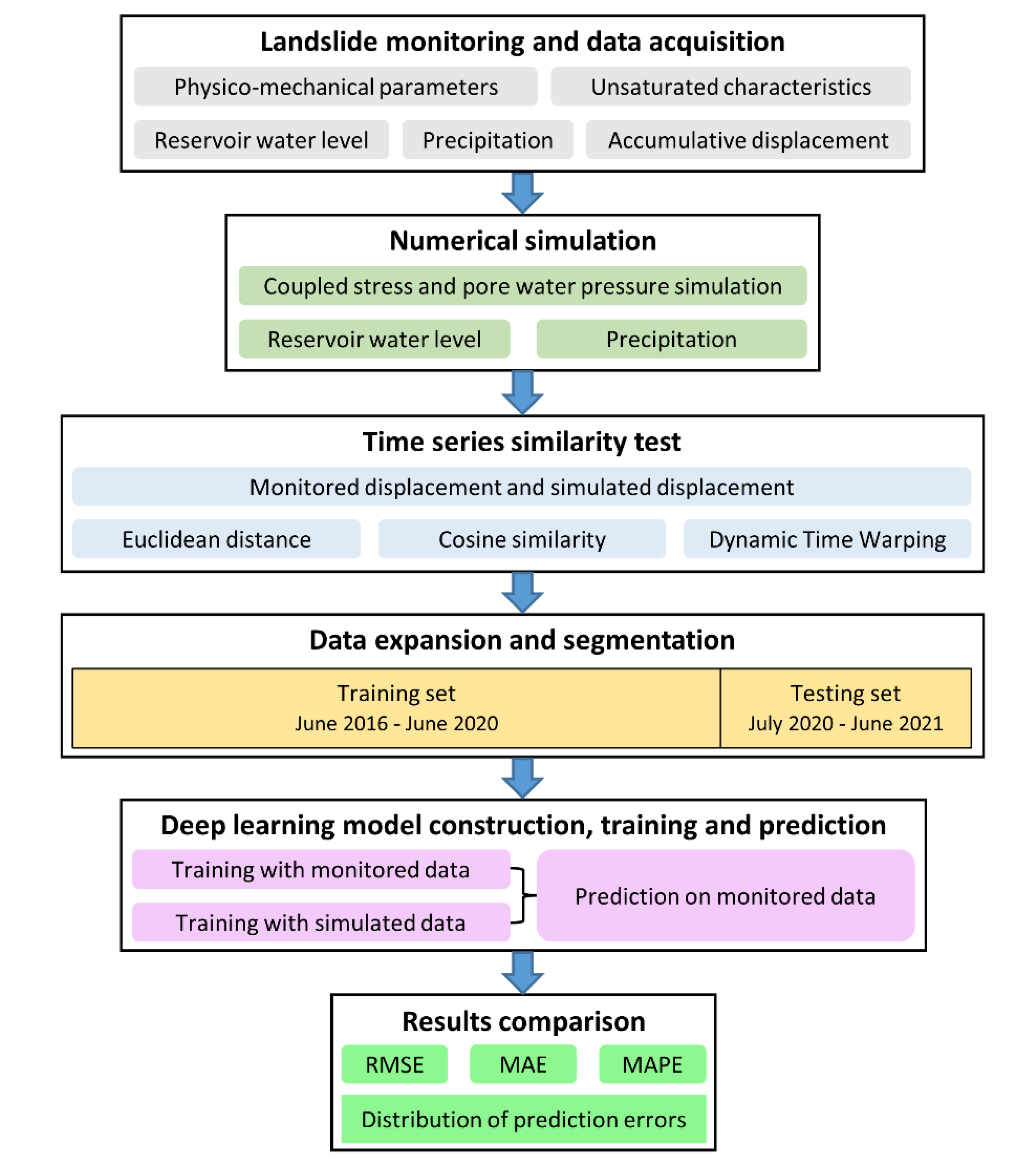
3. Coupled Numerical Simulation Schemes

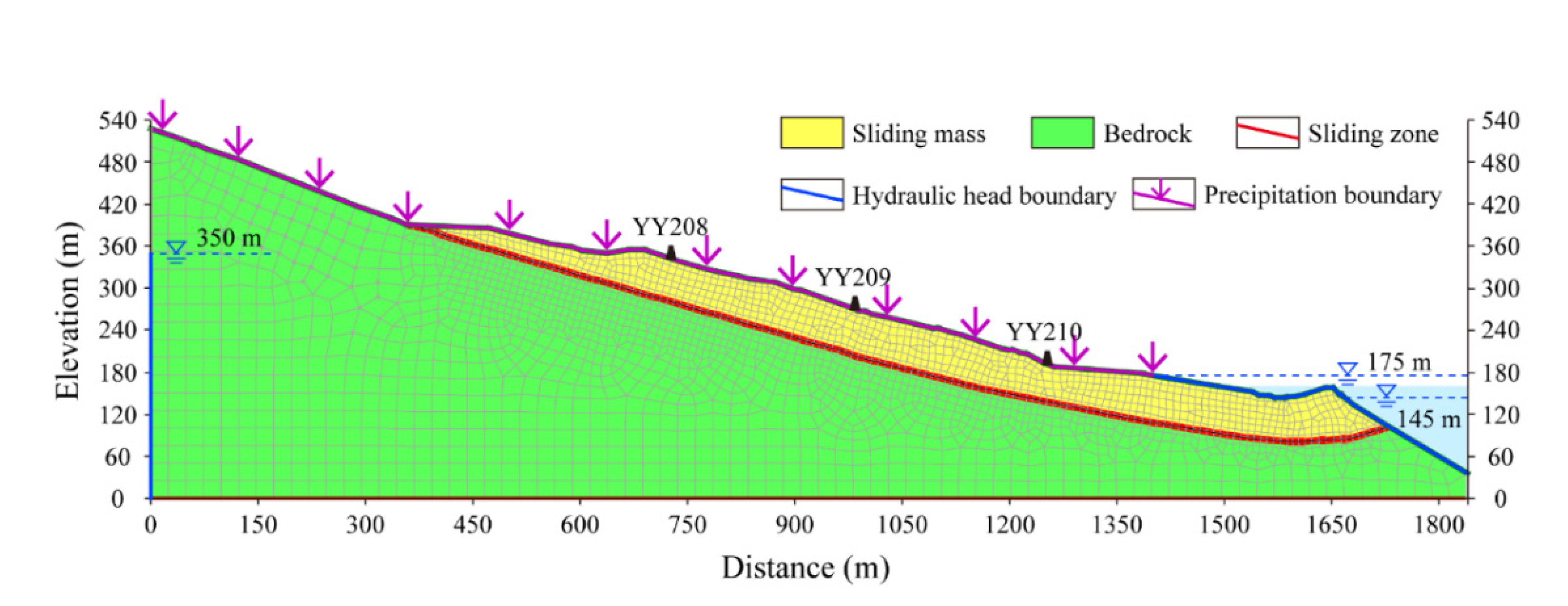
3.1. Numerical Model

The changes in the stress and seepage fields of the Jiuxianping landslide under the action of the cyclic rise and fall of the reservoir water level and rainfall were simulated using SIGMA/W, the 2D finite element stress-deformation analysis module of GeoStudio 2018 [44]. Likewise, the II-II′ geological section of the Jiuxianping landslide was selected to build the numerical model. Before proceeding with the coupled stress and pore water pressure simulations, a branch of the SEEP/W module was created to calculate the initial steady state seepage field. Next an in situ analysis branch was created to obtain the initial stress field. The results of these two branches were employed as the initial stress and initial pore water pressure conditions for the coupled stress and pore water pressure calculations [45].

As shown in Figure 6, the established finite element model that consists of the sliding mass, sliding zone and bedrock is divided into 2666 cells and 2771 nodes. The cells in the bedrock part are slightly sparse, and the cells in the sliding zone and sliding mass parts are suitably refined. This model simplifies the surface clay blanket and the stable accumulation at the back of the landslide. The model’s stress–strain boundary conditions include displacement constraints in the x direction for the left and right boundaries, and displacement constraints in the x and y directions for the lower boundary. The model’s hydraulic boundary conditions include a variable head boundary below the elevation of 175 m on the ground surface of the model for simulating reservoir levels, a variable flow boundary above the model’s surface elevation of 175 m for simulating precipitation, and a constant head of 350 m on the left boundary of the model.

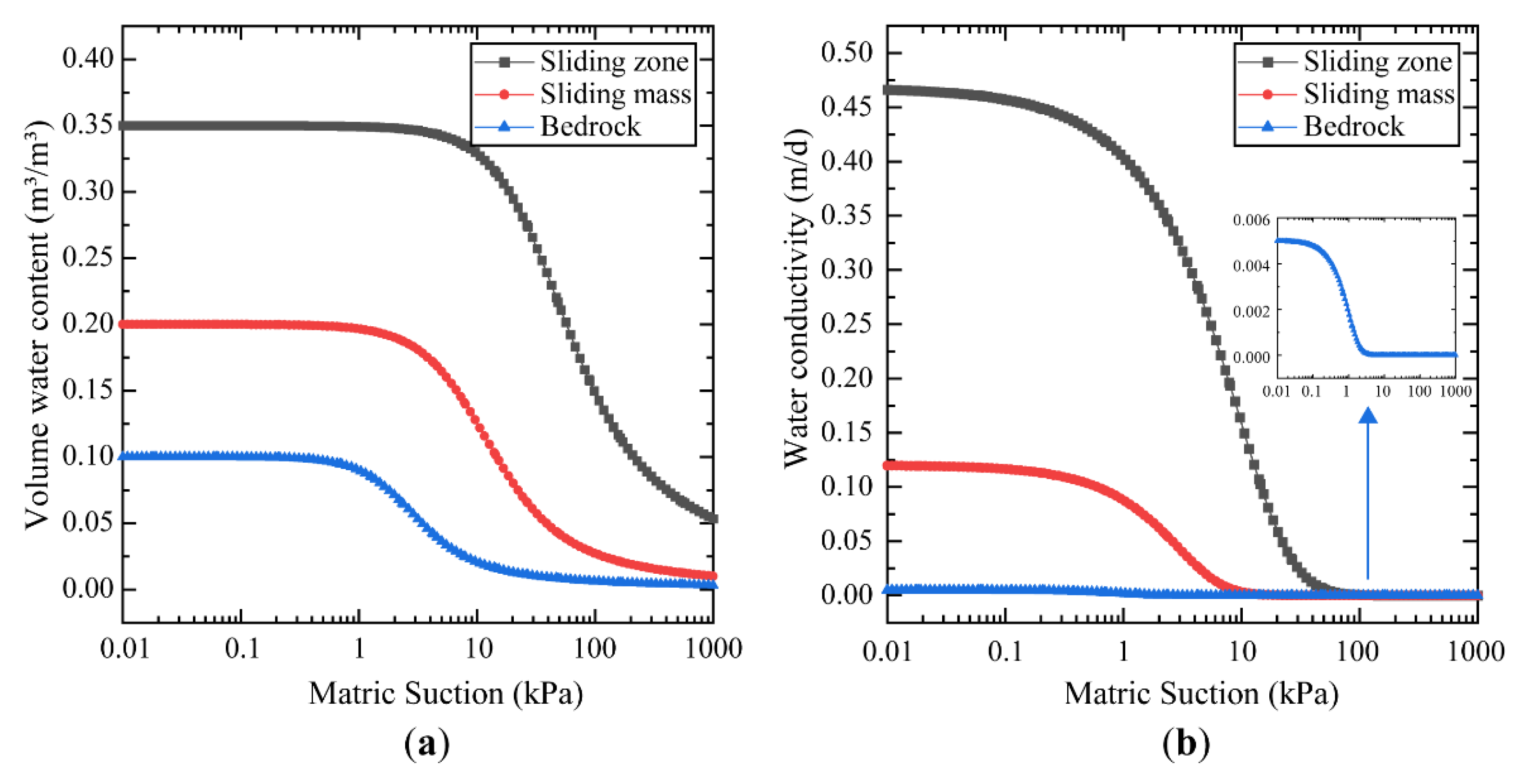
3.2. Simulation Schemes and Parameters

The soil-water characteristic curve (SWCC) and the hydraulic conductivity function (HCF) are important components of the analysis of the saturated–unsaturated medium mechanics. Using GeoStudio’s existing sample functions, the SWCC of the landslide body can be estimated by testing the saturated water content. With the SWCC obtained, the HCF can be estimated in GeoStudio software based on the Van Genuchten method [46] by testing the saturated permeability and the residual volume water content of the landslide materials. The Van Genuchten model can be expressed in Equations (1) and (2).

$$k_w=k_s\frac{{\left\{1-{\left(a\psi \right)}^{n-1}\cdot {\left[1+{\left(a\psi \right)}^n\right]}^{-m}\right\}}^2}{{\left[1+{\left(a\psi \right)}^n\right]}^{m/2}}$$

(1)

$$m=1-\frac{1}{n}$$

(2)

where $k_w$ represents the hydraulic conductivity, $k_s$ represents the saturated hydraulic conductivity, $\psi$ is the range of the matric suction, and $a$, $m$, and $n$ are all curve-fitting parameters. The SWCC and HCF of the Jiuxianping landslide materials are shown in Figure 7; the physico-mechanical properties and permeability coefficients of the materials are shown in

Table 1. Main parameters of the landslide materials used in numerical simulation.

Materials	Unit Weight (kN/m3)	Elastic Modulus (MPa)	Cohesion (kPa)	Poisson Ratio	Friction Angle (°)	Permeability Coefficient (m/d)
Sliding mass	23.8	306	800	0.25	33.9	0.12
Sliding zone	18.4	12.5	20.2	0.28	18	0.468
Bedrock	25.2	1120	-	0.22	-	0.005

. The stress of the sliding zone and sliding mass were calculated using the Mohr–Coulomb yielding criterion, and the linear elastic model was applied to the calculation of the bedrock, due to its small deformation. All material parameters were selected according to the geological investigations and indoor tests; values from the relevant literature were also consulted [47,48,49,50].

The numerical simulation test was conducted based on the monitoring data of the Jiuxianping landslide from 1 June 2016 to 1 June 2021. The duration of the simulation was set as 1800 days, and every 30 days was set as a calculation step. A total of 60 displacement series data were calculated in this way, and with the initial 0 displacement, a displacement time series of the length 61 was obtained from the simulation in order to examine the matching degree of the real monitoring displacement and simulated displacement. Considering that the reservoir level had just experienced a rapid drawdown when monitoring first started (1 June 2016), the head boundary for calculating the steady state seepage field was thus set as 160 m. The reservoir level and precipitation used in the coupled calculations were all the actual observed values, as illustrated in Figure 5.

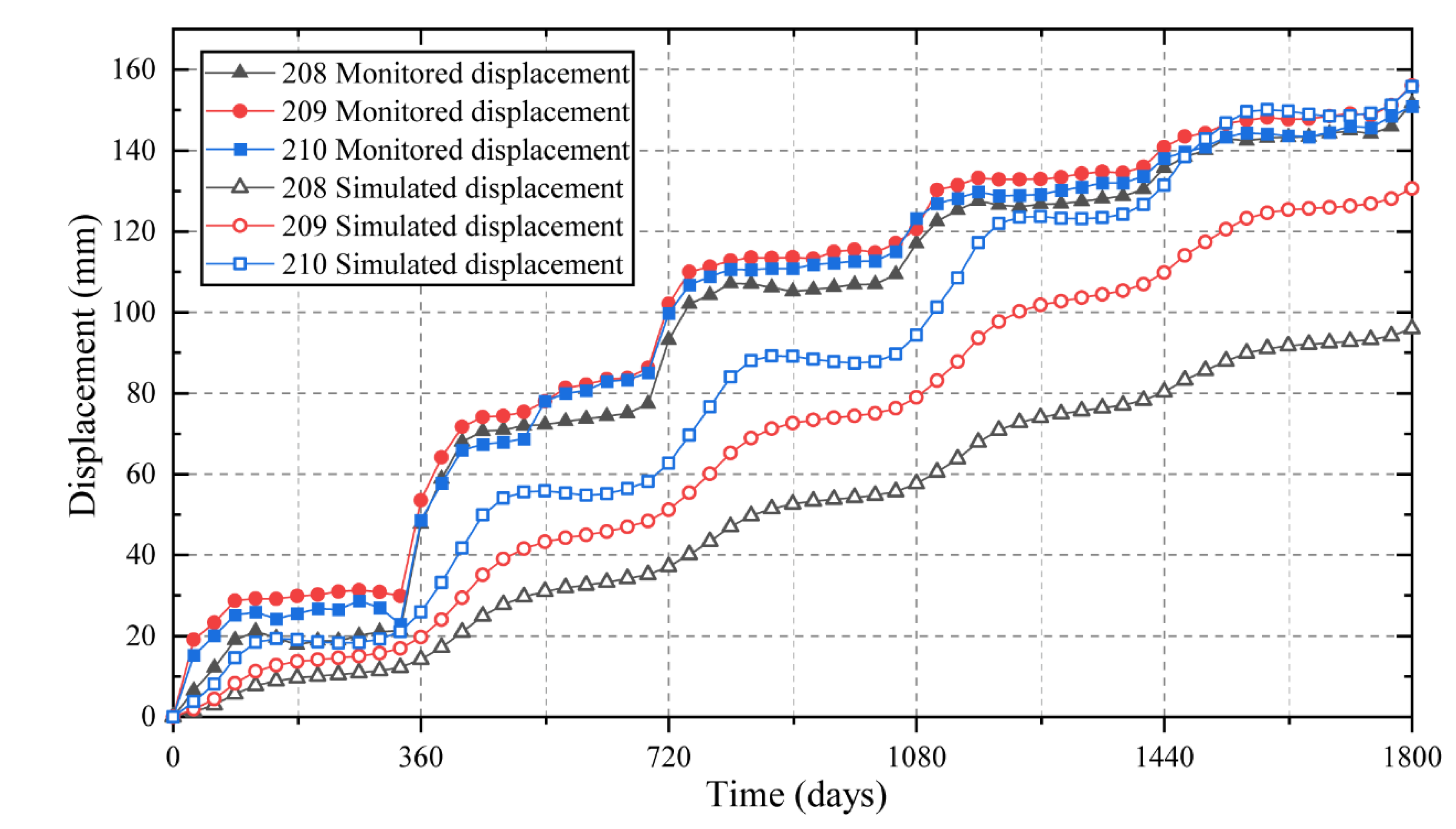
3.3. Simulation Results

For further verification of the validity and reliability of the numerical model, three points on the surface of the model were monitored. The points were located at the elevations of 340 m, 270 m and 190 m, corresponding to the landslide displacement observation points YY208, YY209 and YY210, respectively. Since the accumulated displacement at YY206 and YY207 was quite small, these two points will not be further investigated in this paper. Figure 8 presents the simulation results of the cumulative displacement at the three monitoring points under the coupling effect of rainfall and reservoir water level fluctuations. In addition, the actual measured data are compared with the results of the numerical simulation.

The final cumulative displacements at the three points of the model were 95.97 mm, 130.62 mm, and 155.82 mm under the coupling of rainfall and reservoir water level, respectively. The final cumulative displacements at the monitoring points on the landslide surface were 151.64 mm, 156.10 mm, and 150.90 mm, respectively. It can be seen that the actual displacement of the Jiuxianping landslide is in fact relatively consistent at all points, with the actual cumulative displacements at YY208, YY209 and YY210 all between 150–160 mm. From the numerical simulation results, the final cumulative displacement at YY210 is more consistent with the actual, with the same five rising stages and five calmer stages, while the simulated displacements at YY208 and YY209 are both smaller than the actual.

The precipitation and reservoir level fluctuations change the seepage field of the slope, and the change in the seepage field leads to the change in pore water pressure in the slope [51]. Figure 9 shows the pore water pressure of the Jiuxianping landslide during a 360-day period in the numerical simulation. From the results of numerical simulation, the pore water pressure changes in the landslide during the period are mainly concentrated in the front part, which is influenced by the rise and fall of reservoir water level, and not significantly influenced by rainfall. One report in the literature [52] elaborates the deformation mechanism of TGRA landslides influenced by reservoir water level. When the reservoir water level rises, the buoyancy force increases, and the pore water pressure of the area below the water level of the front edge of the landslide increases, producing a dynamic water pressure that points towards the slope, also called seepage force, preventing the slide of the landslide and increasing its stability. When the reservoir water level falls, this dynamic water pressure becomes directed outward on the slope, reducing the strength of the sliding zone and the structural surfaces, causing the rock mass to slide as a whole under the action of gravity. In the numerical simulation software, the further away from the bank, the less the seepage field changes, the less the pore water pressures are affected and the less the deformation that occurs. This is the reason why the simulated cumulative displacements at YY209 and YY210 points are smaller than the real value.

Although the numerical simulation did not achieve the strict overall deformation of the landslide, it can be noted that the simulated displacement at point YY210 was very close to the real displacement curve and can be considered for further study based on the simulated displacement at this point.

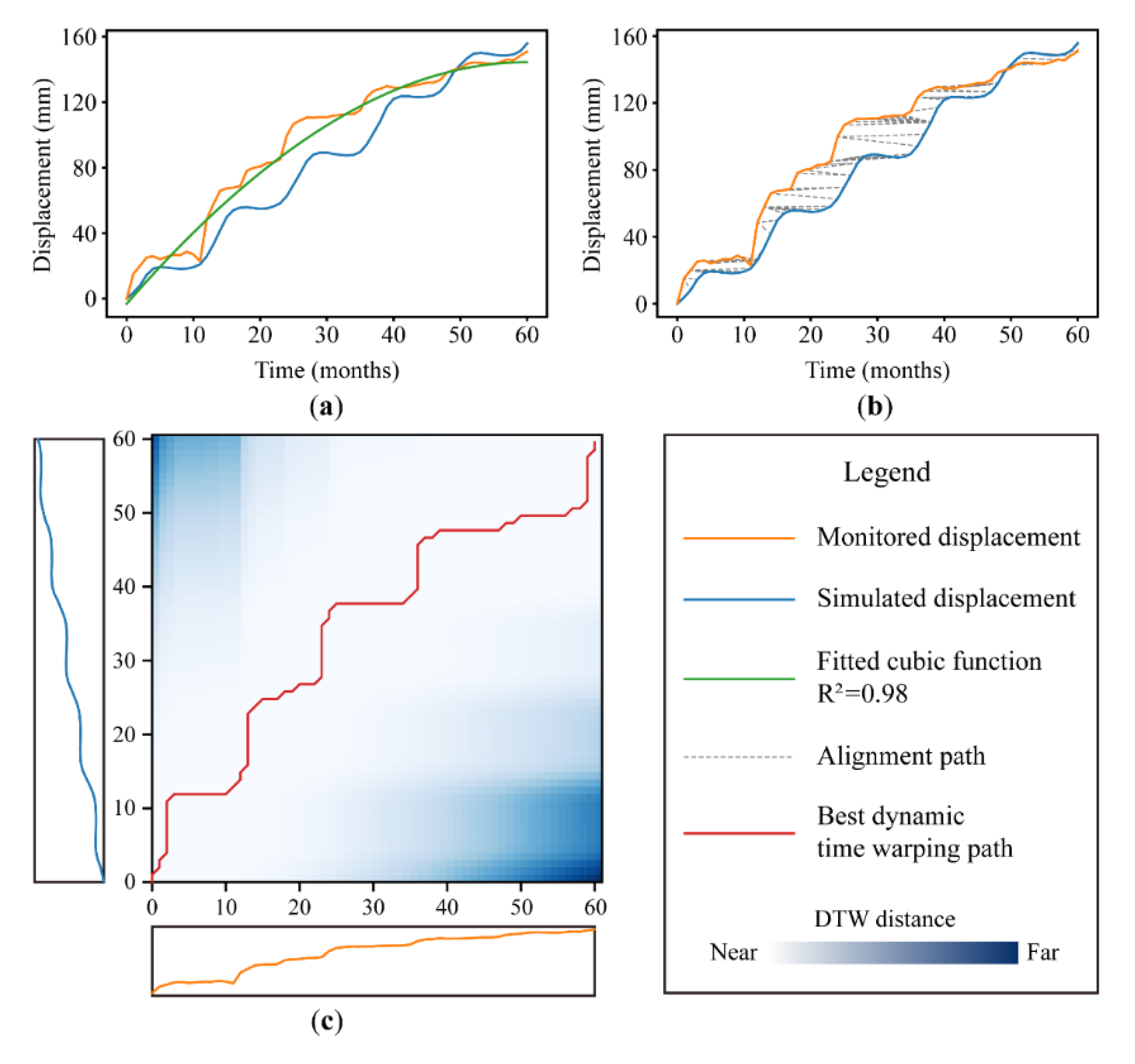
4. Displacement Time Series Similarity

Numerical simulations were carried out in the previous section to obtain displacement data of equal length to the actual monitoring data. It is evident that both the displacement data obtained after monitoring and that obtained after simulation are in accordance with the characteristics of time series. To investigate how close the simulated and measured data from monitoring site YY210 are in terms of time series, several methods and metrics will be used in this section to examine the similarity and correlation between the simulated and actual monitoring displacement time series data.

4.1. Numerical Similarity

First, we want to know how similar the two time series are numerically, a problem that can also be understood as how far apart each of the points in the sequences are in the two-dimensional plane. To measure the distance between points, the Euclidean distance is a useful metric that is widely applied in many fields [53,54,55]. The Euclidean distance is derived from the Minkowski distance, first proposed by the mathematician Hermann Minkowski. Suppose there are two time series $P=\left(x_1,x_2,\dots ,x_n\right)$ and $Q=\left(y_1,y_2,\dots ,y_n\right)$ in an n-dimensional space; then, the Minkowski distance can be expressed in Equation (3).

$$D_M\left(P,Q\right)={\left({\displaystyle \sum }_{i=1}^n{\left|x_i-y_i\right|}^p\right)}^{\frac{1}{p}}$$

(3)

where $p$ is a constant, and the Manhattan distance is obtained for $p=1$, the Euclidean distance for $p=2$, and the Chebyshev distance when $p$ tends to infinity. So, the Euclidean distance is defined in Equation (4). The smaller the Euclidean distance, the better the numerical similarity of the two time series.

$$D_E\left(P,Q\right)=\sqrt{{\displaystyle \sum }_{i=1}^n{\left(x_i-y_i\right)}^2}$$

(4)

A simple calculation gave an average Euclidean distance of 14.39 mm for the two time series data; that is, the average error of the displacement obtained from the simulation was about 9%.

4.2. Orientation Similarity

In addition to wanting shorter distances at each point, we also expect the two series curves to have a similar trend, which means that the curves rise or fall at the same time. The cosine similarity focuses more on the difference between two vectors in terms of direction rather than distance. Placing the points of the two time series in a plane coordinate system, the line between each point and the origin of the coordinate axis is a vector. The cosine of the angle between every two vectors can represent their cosine similarity. Given two time series $P=\left(x_1,x_2,\dots ,x_n\right)$ and $Q=\left(y_1,y_2,\dots ,y_n\right)$, their cosine similarity can be defined as:

$$D_{cos}\left(P,Q\right)=\frac{{{\displaystyle \sum }}_{i=1}^n{x}_i{y}_i}{\sqrt{{{\displaystyle \sum }}_{i=1}^n{x}_i^2}\sqrt{{{\displaystyle \sum }}_{i=1}^n{y}_i^2}}$$

(5)

The closer the cosine is to 1, the higher the cosine similarity of the two series data, which means that they are more consistent in their orientations. The average cosine similarity between the simulated and monitored displacement time series was calculated to be 0.989, which indicates that they are highly similar in direction.

4.3. Shape Similarity

As can be seen, for time series similarity measurements, the Euclidean distance-based metric is insensitive to the shapes of the series, and the cosine similarity-based metric is powerless to calculate the distance between points. Consider a simple but integrated approach to measuring the similarity of these two time series, the dynamic time warping (DTW) method. DTW was proposed by Japanese scholar Itakura in the 1960s [56]. This algorithm is based on the idea of dynamic programming, which solves the problems of speech template matching, being one of the most popular algorithms in the speech recognition field.

DTW is a dynamic programming method that minimizes the distance between two sequences by finding the smallest alignment matching path; thus, DTW can calculate distances for sequences of different lengths, avoiding the problems that might occur with time series offsets [57]. Given two time series (the two time series are not necessarily of equal length, m and n are not necessarily equal) $P=\left(x_1,x_2,\dots ,x_m\right)$ and $Q=\left(y_1,y_2,\dots ,y_n\right)$, let $A_{m\times n}={\left(a_{ij}\right)}_{m\times n}$ denote the distance matrix of $P$ and $Q$, where $a_{ij}$ is calculated based on the distance metric, usually using the square of the Euclidean distance:

$$a_{ij}={\left(x_i-y_j\right)}^2$$

(6)

The ultimate goal of the dynamic programming method is to find a path through a number of grid points in the grid, and the grid points through which the path passes are the points where the two sequences are aligned for calculation. Defining $W=w_1,w_2,\dots ,w_k$ as the dynamic time warping path between the time series $P$ and $Q$, where $w_k={\left(a_{ij}\right)}_k$ is the k-th element of the path, then the path $W$ needs to satisfy the following conditions:

$$\left\{\begin{array}{l}\max \left\{m,n\right\}\le K\le m+n-1\hfill \\ w_1=a_{11},w_k=a_{mn}\hfill \\ 0\le k-i\le 1, 0\le l-j\le 1 \left(\mathrm{if} w_k=a_{ij} \mathrm{and}{w}_{k+1}=a_{kl}\right)\hfill \end{array}\right.$$

(7)

Obviously, the dynamic time warping path is not unique. The path that has the minimum value of $\sqrt{{\displaystyle \sum }_{i=1}^k{w}_i}$ among all of the dynamic time warping paths is called the best dynamic time warping path, and the corresponding distance is the dynamic time warping distance. Defining $DTW\left(P,Q\right)$ as the DTW distance between $P$ and $Q$, then it follows that:

$$DTW\left(P,Q\right)=\min \left(\sqrt{{\displaystyle \sum }_{i=1}^k{w}_i}\right)$$

(8)

In addition, this part also adopts two metrics, root mean square error (RMSE) and mean absolute error (MAE) for comparison.

$$\mathrm{RMSE}=\sqrt{\frac{1}{n}{\displaystyle \sum }_{i=1}^n{({\widehat{y}}_i-y_i)}^2}$$

(9)

$$\mathrm{MAE}=\frac{1}{n}{\displaystyle \sum }_{i=1}^n\left|{\widehat{y}}_i-y_i\right|$$

(10)

where, $n$ represents the sample size, and $y_i$ and ${\widehat{y}}_i$ are the monitored displacement and simulated displacement (or fitted data), respectively. The smaller the metrics, the higher the similarity between the evaluated objects.

The results of the similarity evaluation based on the DTW method are summarized in Figure 10 and

Table 2. Root mean square error (RMSE), mean absolute error (MAE) and DTW distance between the curves.

Metric	RMSE (mm)	MAE (mm)	DTW Distance (mm)
Monitored-Simulated	17.58	14.39	633.47
Monitored-Fitted	6.91	5.06	642.84

. To demonstrate the DTW similarity between the simulated and monitored displacements, a fitted curve of the cubic function of the monitored displacements was added as a comparison (Figure 10a). The expression of this fitted cubic function is $y=-0.00007x^3-0.0328x^2+4.6788x-3.1025$, and its coefficient of determination is $R^2=0.98$. Figure 10b shows the alignment paths of the two displacement curves. The red line in Figure 10c represents the best dynamical time warping path between the monitored and simulated displacement curves. Because of the constraints of Equation (7), it can only be extended to the right, up, and to the upper right.

As can be seen from the results presented in Table 2, the RMSE and MAE between the fitted function curve and the monitored displacement are 6.91 mm and 5.06 mm, respectively, which are much smaller than the RMSE and MAE between the simulated displacement and the monitored displacement. However, the evaluation method based on the DTW distance gives a completely different result. The total DTW distance between the fitted function curve and the monitored displacement is 642.84 mm, which is even slightly higher than the total DTW distance between the simulated and monitored displacements of 633.47 mm. Such results indicate that, from a dynamic programming perspective, there is a higher shape similarity between the simulated and monitored displacement curves than between the fitted and monitored displacements. This demonstrates, to some extent, the high feasibility of machine learning modeling and calculation by using simulated displacement time series data instead of measured displacement data, as there is a high level of similarity between them in terms of time series.

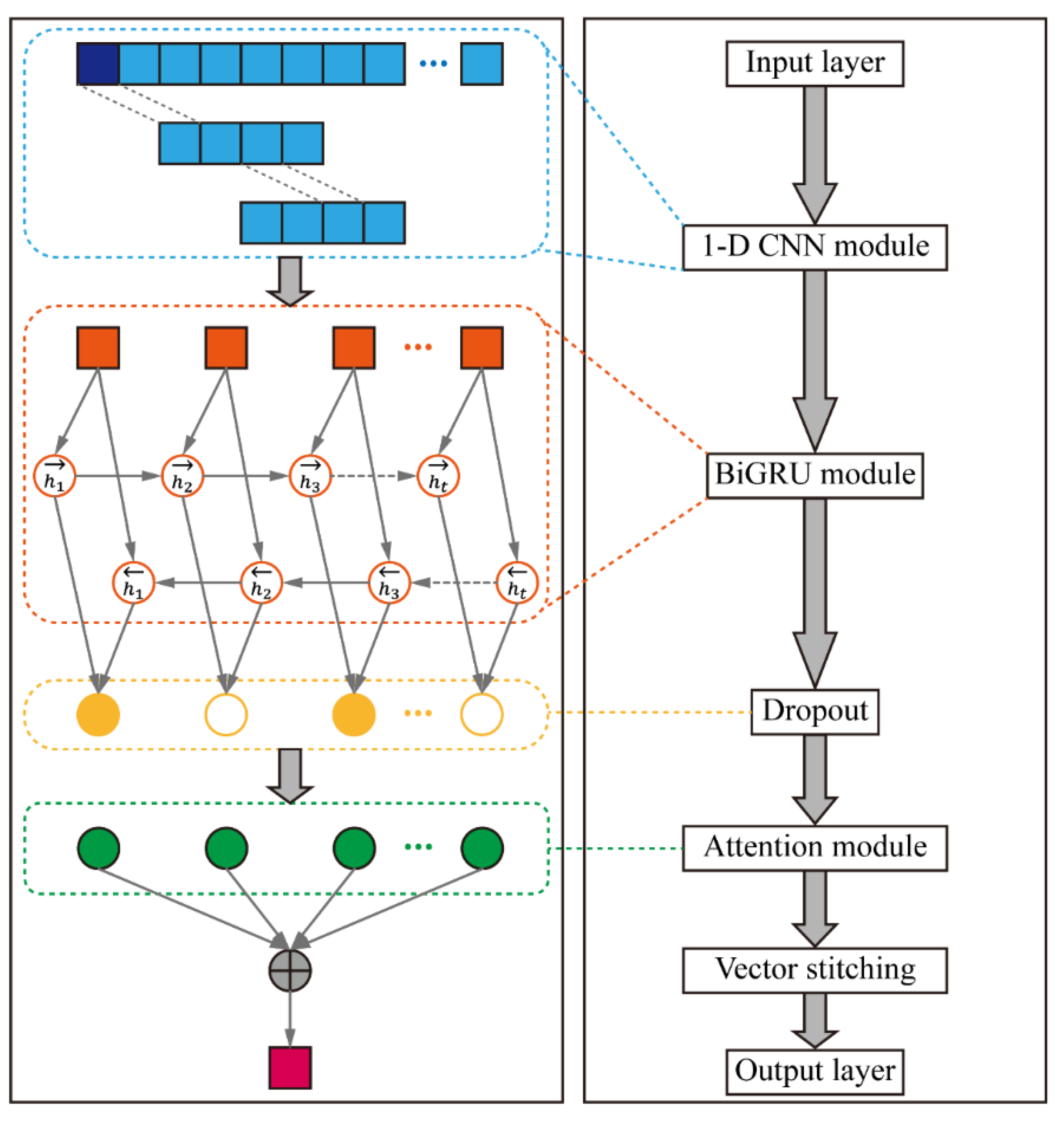
5. Displacement Prediction Deep Learning Model

Long-term landslide displacement monitoring can acquire a large amount of slope surface deformation data. The time series data obtained are nonlinear and dynamic, and the predicted data are inextricably linked not only to the inputs to the system at the current moment, but also to the inputs to the system in the past. Considering the dynamic and non-linear nature of landslide evolution, this study proposes a deep learning model coupled with the one-dimensional (1-D) convolutional neural network (CNN), bidirectional gate recurrent unit (BiGRU), and attention mechanism (AM) to mine and predict the acquired landslide displacement data. The architecture of the CNN-BiGRU-AM deep learning model is displayed in Figure 11.

5.1. Deep Learning Model Construction

5.1.1. CNN Module

For time series data, this study first extracts local features from the displacement data using a 1-D CNN, which consists of a convolutional layer, a pooling layer and a fully connected layer. The model first uses a convolutional kernel for feature extraction, followed by a rectified linear units (ReLU) function for activation and a max-pooling layer for pooling. The 1-D CNN outputs a sequence of data as input to the BiGRU module. The convolution and pooling layers are calculated based on the following equations.

$${\mathit{c}}_i=f\left({\mathit{\omega }}_i{\mathit{x}}_i+{\mathit{b}}_i\right)$$

(11)

$${\mathit{p}}_i=\max \left({\mathit{c}}_i\right)$$

(12)

where ${\mathit{c}}_i$ represents the output of the convolutional layer, $f\left(\bullet \right)$ represents the activation function, ${\mathit{x}}_i$ is the input of the convolutional layer, ${\mathit{\omega }}_i$ is the weight, ${\mathit{b}}_i$ is the bias, and ${\mathit{p}}_i$ is the output of the max-pooling layer.

5.1.2. BiGRU Module

The recurrent neural network (RNN) is suitable for processing time series data because of the unique memory units. However, RNN suffers from gradient disappearance and gradient explosion when dealing with long sequences. Many variants of RNN have since emerged, such as LSTM and GRU [58,59,60], and GRU is simpler in structure and faster in training than LSTM. Instead of introducing an additional memory unit, it introduces an update gate to control how much information the current state ${\mathit{h}}_t$ needs to retain from the previous state, and how much new information it needs to receive from the candidate state. ${\mathit{h}}_t$ can be expressed as:

$${\mathit{h}}_t={\mathit{z}}_t\odot {\mathit{h}}_{t-1}+\left(1-{\mathit{z}}_t\right)\odot \mathrm{g}\left({\mathit{x}}_t,{\mathit{h}}_{t-1};\theta \right)$$

(13)

where ${\mathit{z}}_t\in {\left[0,1\right]}^D$ is the update gate.

$${\mathit{z}}_t=\mathsf{\sigma }\left({\mathit{W}}_z{\mathit{x}}_t+{\mathit{U}}_z{\mathit{h}}_{t-1}+{\mathit{b}}_z\right)$$

(14)

The GRU uses only one gate in place of the input and forgetting gates. In GRU, the function $\mathrm{g}\left({\mathit{x}}_t,{\mathit{h}}_{t-1};\theta \right)$ is defined as:

$${\tilde{\mathit{h}}}_t=\tanh \left({\mathit{W}}_h{\mathit{x}}_t+{\mathit{U}}_h\left({\mathit{r}}_t\odot {\mathit{h}}_{t-1}\right)+{\mathit{b}}_h\right)$$

(15)

where ${\tilde{\mathit{h}}}_t$ indicates the candidate state at the current moment, and ${\mathit{r}}_t\in {\left[0,1\right]}^D$ is the reset gate. ${\mathit{r}}_t$ is used to control whether the calculation of the candidate state ${\tilde{\mathit{h}}}_t$ depends on the state ${\mathit{h}}_{t-1}$ at the previous moment. In summary, the state of the GRU network is updated in the following way:

$${\mathit{h}}_t={\mathit{z}}_t\odot {\mathit{h}}_{t-1}+\left(1-{\mathit{z}}_t\right)\odot {\tilde{\mathit{h}}}_t$$

(16)

BiGRU consists of two GRU networks with the same inputs, only the information is passed in different directions. This structure enhances its ability to address nonlinear time series, and allows for more sufficient training. The hidden state of the BiGRU at moment $t$ is defined as:

$${\mathit{h}}_t=\overrightarrow{{\mathit{h}}_t}\oplus \overleftarrow{{\mathit{h}}_t}$$

(17)

where, $\overrightarrow{{\mathit{h}}_t}$ and $\overleftarrow{{\mathit{h}}_t}$ are the hidden states of the forward and backward GRUs, respectively, at moment $t$, $\oplus$ represents the stitching of vectors.

5.1.3. AM Module

The main concept of AM derives from the process of human visual attention [61]. When faced with a long sequence, the model focuses on the important parts of the input sequence and ignores the minor parts by introducing AM to achieve better results than a model without attention. The output of the attention layer is defined using the following equations:

$$M=Sigmoid\left({\mathit{o}}_t\right)$$

(18)

$$\alpha =softmax\left({\omega }^{T}M\right)$$

(19)

$$O={\mathit{o}}_t{\alpha }^T$$

(20)

where ${\mathit{o}}_t$ is the output of the BiGRU, which is transformed by the sigmoid function with weights ${\omega }^T$ weighted and summed through $softmax$ output to obtain $\alpha$ as the coefficient of attention. At last, $\alpha$ and ${\mathit{o}}_t$ are multiplied to obtain the attention value $O$.

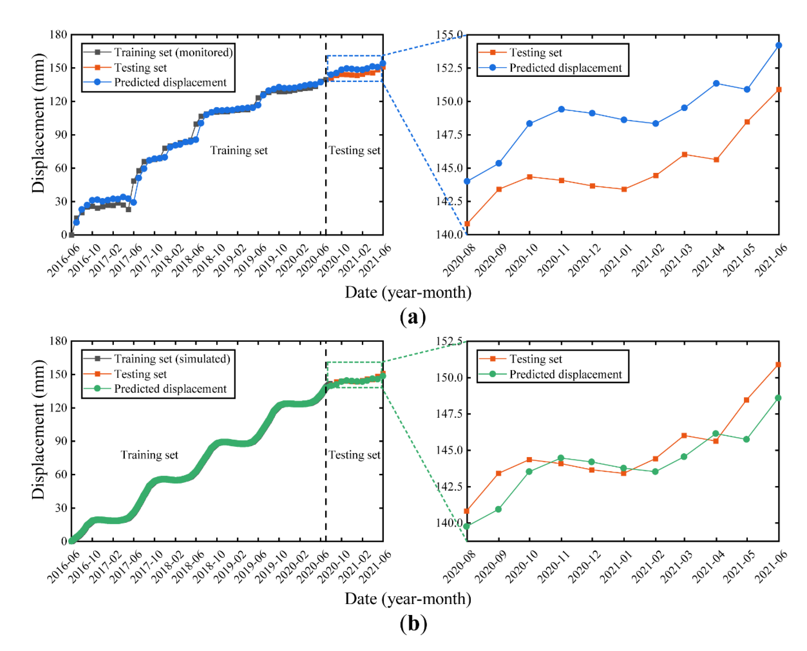
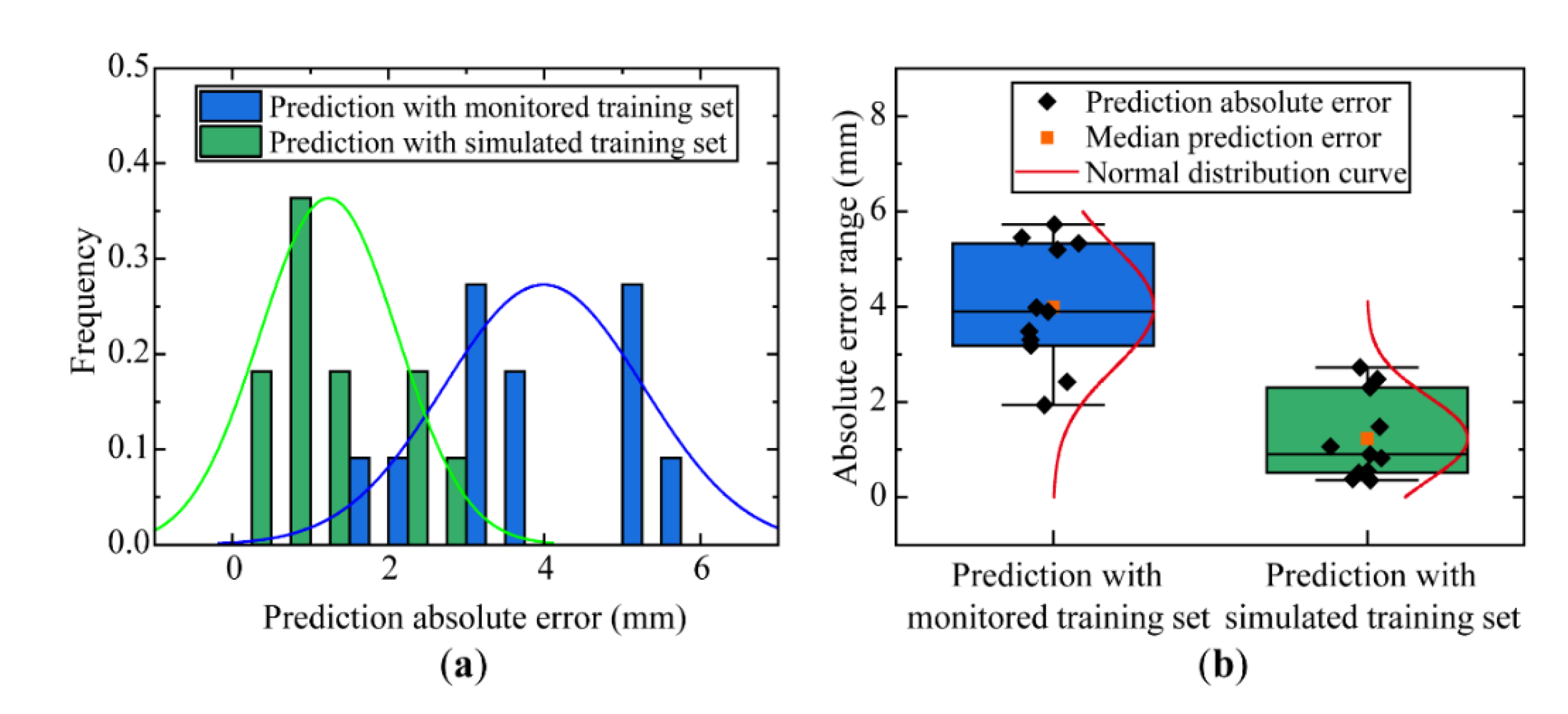
5.2. Model Training and Prediction

The coupled CNN-BiGRU-AM deep learning model in this study was built and trained using the deep learning library Keras. The training samples of the model were derived from the displacement data of 1800 days in the numerical simulation. By setting every single day as a step and saving the data of each step, a displacement time series with a length of 1801 including the initial zero displacement was obtained. To prove the benefits of training based on numerical simulation data, the results of training and prediction based on actual measured data were also added for comparison. As shown in

Table 3. Division of training set and testing set.

Data Set		Date Span	Data Length
Training set	Monitored data	June 2016–June 2020	1470
	Simulated data	June 2016–June 2020	49
Testing set	Monitored data	July 2020–June 2021	12

, when training with monitored displacement data, the training set was the first 49 points of the monitored data. When training with simulated displacement data, the training set was the first 1470 points of the simulated data. The date span of the training set data was from June 2016 to June 2020. The last 12 data points of the monitored displacements were set as the common testing set, spanning the dates from July 2020 to June 2021, representing approximately 20% of the entire monitored data set.

Partial hyperparameters used for model training are shown in

Table 4. Partial hyperparameters for two training tasks.

Hyperparameter	Dropout	Batch Size	Filter Length	GRU Units
Training with monitored data	0	16	4	32
Training with simulated data	0.1	64	4	32

. Since the size of the training sets differed between the two tasks, the hyperparameters used for the two training missions were slightly different. The hyperparameters used were designed to make the model as optimal as possible. When training with simulated displacement data, a dropout module with a factor of 0.1 was added to prevent overfitting. The optimization metric for the training task was the MSE between predicted values and targets, and the training optimizer used the Adam algorithm. A one-step prediction method was used to predict the displacement at the next moment.

In addition to RMSE and MAE mentioned in Section 4, MAPE will also be used as an evaluation metric for displacement prediction accuracy in this section. The MAPE metric can be calculated by Equation (21).

$$\mathrm{MAPE}=\frac{1}{n}{\displaystyle \sum }_{i=1}^n\left|\frac{{\widehat{y}}_i-y_i}{y_i}\right|\times 100\%$$

(21)

where $n$ represents the sample size, $y_i$ and ${\widehat{y}}_i$ are the monitoring and predicted values respectively. The results and predicted errors of the proposed deep learning model, which was trained by monitored and simulated displacements, respectively, and tested by monitored displacement, are shown in Figure 12 and

Table 5. Errors of the predicted displacement with CNN-BiGRU-AM.

Metric	MAE (mm)	RMSE (mm)	MAPE (%)
Prediction with monitored training set	3.99	4.17	2.68
Prediction with simulated training set	1.23	1.50	0.85

.

From Figure 12 it can be observed that the CNN-BiGRU-AM model can predict the trend of the testing set data well after being trained on both the monitored data and the simulated data. The difference is that the models trained with data from numerical simulations are more accurate than those trained with actual monitored data, since the predicted displacement curve based on the simulated data set is closer to the measured data curve. This is also supported by the error metrics in Table 5. The prediction errors for MAE, RMSE and MAPE with the monitored training set were 3.99 mm, 4.17 mm and 2.68%, respectively, while the prediction errors for MAE, RMSE and MAPE with the simulated training set were 1.23 mm, 1.50 mm and 0.85%, respectively. It is clear that the displacement data obtained from the numerical simulations are not only reliable, but also help to train the model to significantly reduce prediction errors.

Figure 13 provides the absolute error distribution of the predicted values. Figure 13a provides the frequency distribution of the prediction errors. Most of the prediction errors obtained based on the simulated dataset were less than 2 mm, while the prediction errors obtained based on the monitoring dataset training were basically in the range of 2–6 mm. In Figure 13b, the box plot gives the interquartile range of the prediction errors; the orange points indicate the median value of the errors and the red curve is the fitted normal distribution curve of the errors. When model training is carried out using the training dataset generated by numerical simulation, it results in a more concentrated statistical distribution of prediction errors.

It is noted that not much effort was spent on hyperparameter optimization of the model in this study. We believe that the deep learning model will achieve more satisfactory results if the parameters are optimized specifically. Moreover, the purpose of this paper was to investigate the feasibility and precision of using numerical simulation to obtain a big data set for deep learning, so only displacement time series were considered. If more geological observation data can be integrated for the model training, the displacement prediction results will be more accurate.

6. Discussion

We demonstrated a prediction method for landslide displacement combining numerical simulation and deep learning methods in this paper. Aiming at the lack of big data volume in the field of geological hazard prediction such as landslides, this study explored the scientificity and feasibility of expanding the deep learning dataset using numerical simulation. We built a finite element numerical model considering the real precipitation and reservoir level conditions, and this model was used to generate and expand the training set required for the deep learning model. The results suggest that this is an effective method for augmenting finite data and is superior to conventional, mathematically based interpolation methods because of its interpretability of mechanism. In practical engineering applications, we believe that the proposed method can solve the following problems: (1) the small amount of monitoring data obtained when the frequency of field monitoring is low, potentially resulting in models insufficiently trained with an inadequate training set; and (2) the problem of missing monitoring data or abnormal data that is often caused by equipment or personnel problems during monitoring.

This study is a preliminary attempt to combine numerical simulation with deep learning and apply it to landslide hazard prediction, and the authors believe that there are still some aspects to be improved and worthy of deeper exploration. Firstly, the numerical model in this paper is constructed only based on one geological section, and the limited monitoring points can hardly reflect the global trend of landslides. In addition, there is still a certain deviation between the landslide displacement given in the numerical simulation and the actual monitoring displacement, and it is difficult to estimate the strength change of the landslide materials over time, which will affect the precision of the numerical simulation. The environmental triggers of the landslide are not taken into consideration as inputs of the deep learning model, which also has an influence on the accuracy of landslide displacement prediction.

7. Conclusions

In order to solve the problem presented by a small amount of effective landslide monitoring data in practice, we first adopted a mechanism-based approach to expand the limited landslide displacement monitoring data. Utilizing the geotechnical engineering software GeoStudio, a finite element model with coupled pore water pressure was used to conduct numerical simulations of the Jiuxianping landslide. The reservoir water level changes and precipitation over a period of 60 months were considered, and the displacements of the three monitoring points of the landslide during this period were calculated to obtain the corresponding displacement time series data.

The results of the numerical simulations showed that the farther the monitoring point was from the Yangtze River bank, the smaller the accumulated displacement was, and the less obvious the step-like displacement changes were. This can be attributed to the limited influence of changes in the seepage field caused by reservoir level changes in the numerical simulations, whereas in fact the Jiuxianping landslide emerged as a sliding whole.

Three time series similarity metrics—numerical similarity, orientation similarity and shape similarity—were used to evaluate the similarity between the simulated displacement time series and the measured displacement time series at the YY210 point. The numerical similarity based on the mean Euclidean distance, the directional similarity based on the mean cosine value and the shape similarity test based on the DTW distance were 14.39 mm, 0.989 mm and 633.47 mm, respectively, which indicated a high time series similarity between the simulated and measured displacement data of the YY210 monitored point.

Ultimately, a displacement prediction deep learning model for Jiuxianping landslide was constructed. This combined model comprised a 1-D CNN module, a BiGRU module and an attention mechanism, and was supported by 1470 simulation samples extracted from the finite element model. The deep learning model predicted the next moment displacement by mining the historical displacement patterns, and showed good prediction results on a testing set consisting of measured data. For comparison purposes, the original displacement monitoring data were also used for training and testing. The results of the testing set revealed that the model trained on the simulated data had a stronger prediction ability and smaller prediction errors.

References

1. Vu, V.N.; Binh, T.P.; Ba, T.V.; Prakash, I.; Jha, S.; Shahabi, H.; Shirzadi, A.; Dong, N.B.; Kumar, R.; Chatterjee, J.M.; et al. Hybrid Machine Learning Approaches for Landslide Susceptibility Modeling. Forests 2019, 10, 157. [Google Scholar]
2. Catane, S.G.; Veracruz, N.A.S.; Flora, J.R.R.; Go, C.M.M.; Enrera, R.E.; Santos, E.R.U. Mechanism of a low-angle translational block slide: Evidence from the September 2018 Naga landslide, Philippines. Landslides 2019, 16, 1709–1719. [Google Scholar] [CrossRef]
3. Lin, F.; Wu, L.Z.; Huang, R.Q.; Zhang, H. Formation and characteristics of the Xiaoba landslide in Fuquan, Guizhou, China. Landslides 2018, 15, 669–681. [Google Scholar] [CrossRef]
4. Haque, U.; Da Silva, P.F.; Lee, J.; Benz, S.; Auflič, M.J.; Blum, P. Increasing Fatal Landslides in Europe; Springer International Publishing: Cham, Switzerland, 2017; pp. 505–512. [Google Scholar]
5. Sun, D.; Xu, J.; Wen, H.; Wang, D. Assessment of landslide susceptibility mapping based on Bayesian hyperparameter optimization: A comparison between logistic regression and random forest. Eng. Geol. 2021, 281, 105972. [Google Scholar] [CrossRef]
6. Sun, D.; Xu, J.; Wen, H.; Wang, Y. An Optimized Random Forest Model and Its Generalization Ability in Landslide Susceptibility Mapping: Application in Two Areas of Three Gorges Reservoir, China. J. Earth Sci. China 2020, 31, 1068–1086. [Google Scholar] [CrossRef]
7. Guthrie, R.H.; Evans, S.G.; Catane, S.G.; Zarco, M.A.H.; Saturay, R.M., Jr. The 17 February 2006 rock slide-debris avalanche at Guinsaugon Philippines: A synthesis. Bull. Eng. Geol. Environ. 2009, 68, 201–213. [Google Scholar] [CrossRef]
8. Iverson, R.M.; George, D.L.; Allstadt, K.; Reid, M.E.; Collins, B.D.; Vallance, J.W.; Schilling, S.P.; Godt, J.W.; Cannon, C.M.; Magirl, C.S.; et al. Landslide mobility and hazards: Implications of the 2014 Oso disaster. Earth Planet. Sci. Lett. 2015, 412, 197–208. [Google Scholar] [CrossRef] [Green Version]
9. Ouyang, C.; Zhou, K.; Xu, Q.; Yin, J.; Peng, D.; Wang, D.; Li, W. Dynamic analysis and numerical modeling of the 2015 catastrophic landslide of the construction waste landfill at Guangming, Shenzhen, China. Landslides 2017, 14, 705–718. [Google Scholar] [CrossRef]
10. Yang, B.; Yin, K.; Lacasse, S.; Liu, Z. Time series analysis and long short-term memory neural network to predict landslide displacement. Landslides 2019, 16, 677–694. [Google Scholar] [CrossRef]
11. Saito, M. Forecasting Time of Slope Failure by Tertiary Creep; A.A. Balkema: Rotterdam, The Netherlands; Boston, MA, USA, 1969; Volume 2, pp. 677–683. [Google Scholar]
12. Saito, M. Research on Forecasting the Time of Occurrence of Slope Failure; Quarterly Reports; Railway Technical Research Institute: Tokyo, Japan, 1969; Volume 10. [Google Scholar]
13. Crosta, G.B.; Agliardi, F. Failure forecast for large rock slides by surface displacement measurements. Can. Geotech. J. 2003, 40, 176–191. [Google Scholar] [CrossRef]
14. Zvelebill, J.; Moser, M. Monitoring based time-prediction of rock falls: Three case-histories. Phys. Chem. Earth Part B Hydrol. Ocean. Atmos. 2001, 26, 159–167. [Google Scholar] [CrossRef]
15. Rose, N.D.; Hungr, O. Forecasting potential rock slope failure in open pit mines using the inverse-velocity method. Int. J. Rock Mech. Min. 2007, 44, 308–320. [Google Scholar] [CrossRef]
16. Mufundirwa, A.; Fujii, Y.; Kodama, J. A new practical method for prediction of geomechanical failure-time. Int. J. Rock Mech. Min. 2010, 47, 1079–1090. [Google Scholar] [CrossRef] [Green Version]
17. Corominas, J.; Moya, J.; Ledesma, A.; Lloret, A.; Gili, J.A. Prediction of ground displacements and velocities from groundwater level changes at the Vallcebre landslide (Eastern Pyrenees, Spain). Landslides 2005, 2, 83–96. [Google Scholar] [CrossRef]
18. Ma, J.; Tang, H.; Liu, X.; Hu, X.; Sun, M.; Song, Y. Establishment of a deformation forecasting model for a step-like landslide based on decision tree C5.0 and two-step cluster algorithms: A case study in the Three Gorges Reservoir area, China. Landslides 2017, 14, 1275–1281. [Google Scholar] [CrossRef]
19. Lian, C.; Zeng, Z.; Yao, W.; Tang, H.; Chen, C.L.P. Landslide Displacement Prediction with Uncertainty Based on Neural Networks with Random Hidden Weights. IEEE Trans. Neural Netw. Learn. Syst. 2016, 27, 2683–2695. [Google Scholar] [CrossRef] [PubMed]
20. Li, X.Z.; Kong, J.M. Application of GA-SVM method with parameter optimization for landslide development prediction. Nat. Hazards Earth Syst. Sci. 2014, 14, 525–533. [Google Scholar] [CrossRef] [Green Version]
21. Huang, F.; Huang, J.; Jiang, S.; Zhou, C. Landslide displacement prediction based on multivariate chaotic model and extreme learning machine. Eng. Geol. 2017, 218, 173–186. [Google Scholar] [CrossRef]
22. Liu, Z.; Guo, D.; Lacasse, S.; Li, J.; Yang, B.; Choi, J. Algorithms for intelligent prediction of landslide displacements. J. Zhejiang Univ. Sci. A 2020, 21, 412–429. [Google Scholar] [CrossRef]
23. Ma, Z.; Mei, G.; Prezioso, E.; Zhang, Z.; Xu, N. A deep learning approach using graph convolutional networks for slope deformation prediction based on time-series displacement data. Neural Comput. Appl. 2021, 33, 14441–14457. [Google Scholar] [CrossRef]
24. Guo, Z.; Chen, L.; Gui, L.; Du, J.; Yin, K.; Do, H.M. Landslide displacement prediction based on variational mode decomposition and WA-GWO-BP model. Landslides 2020, 17, 567–583. [Google Scholar] [CrossRef]
25. Xu, C.; Dai, F.; Xu, X.; Lee, Y.H. GIS-based support vector machine modeling of earthquake-triggered landslide susceptibility in the Jianjiang River watershed, China. Geomorphology 2012, 145, 70–80. [Google Scholar] [CrossRef]
26. Zhang, L.; Shi, B.; Zhu, H.; Yu, X.B.; Han, H.; Fan, X. PSO-SVM-based deep displacement prediction of Majiagou landslide considering the deformation hysteresis effect. Landslides 2021, 18, 179–193. [Google Scholar] [CrossRef]
27. Zhou, C.; Yin, K.; Cao, Y.; Ahmed, B. Application of time series analysis and PSO-SVM model in predicting the Bazimen landslide in the Three Gorges Reservoir, China. Eng. Geol. 2016, 204, 108–120. [Google Scholar] [CrossRef]
28. Wang, Y.; Tang, H.; Wen, T.; Ma, J. A hybrid intelligent approach for constructing landslide displacement prediction intervals. Appl. Soft Comput. 2019, 81, 105506. [Google Scholar] [CrossRef]
29. Xu, S.; Niu, R. Displacement prediction of Baijiabao landslide based on empirical mode decomposition and long short term memory neural network in Three Gorges area, China. Comput. Geosci. 2018, 111, 87–96. [Google Scholar] [CrossRef]
30. Zhang, W.; Li, H.; Tang, L.; Gu, X.; Wang, L.; Wang, L. Displacement prediction of Jiuxianping landslide using gated recurrent unit (GRU) networks. Acta Geotech. 2022, 17, 1367–1382. [Google Scholar] [CrossRef]
31. Jiang, Y.; Luo, H.; Xu, Q.; Lu, Z.; Liao, L.; Li, H.; Hao, L. A Graph Convolutional Incorporating GRU Network for Landslide Displacement Forecasting Based on Spatiotemporal Analysis of GNSS Observations. Remote Sens. 2022, 14, 1016. [Google Scholar] [CrossRef]
32. Miao, F.; Xie, X.; Wu, Y.; Zhao, F. Data Mining and Deep Learning for Predicting the Displacement of “Step-like” Landslides. Sensors 2022, 22, 481. [Google Scholar] [CrossRef]
33. Wang, H.; Long, G.; Liao, J.; Xu, Y.; Lv, Y. A new hybrid method for establishing point forecasting, interval forecasting, and probabilistic forecasting of landslide displacement. Nat. Hazards 2022, 111, 1479–1505. [Google Scholar] [CrossRef]
34. Xing, Y.; Yue, J.; Chen, C. Interval Estimation of Landslide Displacement Prediction Based on Time Series Decomposition and Long Short-Term Memory Network. IEEE Access 2020, 8, 3187–3196. [Google Scholar] [CrossRef]
35. Li, S.H.; Wu, L.Z.; Chen, J.J.; Huang, R.Q. Multiple data-driven approach for predicting landslide deformation. Landslides 2020, 17, 709–718. [Google Scholar] [CrossRef]
36. Ma, Z.; Mei, G. Deep learning for geological hazards analysis: Data, models, applications, and opportunities. Earth Sci. Rev. 2021, 223, 103858. [Google Scholar] [CrossRef]
37. Yokoya, N.; Yamanoi, K.; He, W.; Baier, G.; Adriano, B.; Miura, H.; Oishi, S. Breaking limits of remote sensing by deep learning from simulated data for flood and debris-flow mapping. IEEE Trans. Geosci. Remote Sens. 2020, 60, 1–15. [Google Scholar] [CrossRef]
38. Xiong, X.; Shi, Z.; Xiong, Y.; Peng, M.; Ma, X.; Zhang, F. Unsaturated slope stability around the Three Gorges Reservoir under various combinations of rainfall and water level fluctuation. Eng. Geol. 2019, 261, 105231. [Google Scholar] [CrossRef]
39. Zhao, N.; Hu, B.; Yi, Q.; Yao, W.; Ma, C. The Coupling Effect of Rainfall and Reservoir Water Level Decline on the Baijiabao Landslide in the Three Gorges Reservoir Area, China. Geofluids 2017, 2017, 3724867. [Google Scholar] [CrossRef] [Green Version]
40. Jiang, J.; Ehret, D.; Xiang, W.; Rohn, J.; Huang, L.; Yan, S.; Bi, R. Numerical simulation of Qiaotou Landslide deformation caused by drawdown of the Three Gorges Reservoir, China. Environ. Earth Sci. 2011, 62, 411–419. [Google Scholar] [CrossRef]
41. Du, J.; Yin, K.; Lacasse, S. Displacement prediction in colluvial landslides, Three Gorges Reservoir, China. Landslides 2013, 10, 203–218. [Google Scholar] [CrossRef]
42. Tang, H.; Wasowski, J.; Juang, C.H. Geohazards in the three Gorges Reservoir Area, China Lessons learned from decades of research. Eng. Geol. 2019, 261, 105267. [Google Scholar] [CrossRef]
43. Yao, W.; Li, C.; Zuo, Q.; Zhan, H.; Criss, R.E. Spatiotemporal deformation characteristics and triggering factors of Baijiabao landslide in Three Gorges Reservoir region, China. Geomorphology 2019, 343, 34–47. [Google Scholar] [CrossRef]
44. GEOSLOPE International Ltd. Static Stress-Strain Modeling with GeoStudio; GEOSLOPE International Ltd.: Calgary, AB, Canada, 2021. [Google Scholar]
45. GEOSLOPE International Ltd. Rapid Drawdown; GEOSLOPE International Ltd.: Calgary, AB, Canada, 2018. [Google Scholar]
46. Van Genuchten, M.T. A closed-form equation for predicting the hydraulic conductivity of unsaturated soils. Soil Sci. Soc. Am. J. 1980, 44, 892–898. [Google Scholar] [CrossRef] [Green Version]
47. Hu, X.; He, C.; Zhou, C.; Xu, C.; Zhang, H.; Wang, Q.; Wu, S. Model Test and Numerical Analysis on the Deformation and Stability of a Landslide Subjected to Reservoir Filling. Geofluids 2019, 2019, 5924580. [Google Scholar] [CrossRef] [Green Version]
48. Zhao, N.; Hu, B.; Yan, E.; Xu, X.; Yi, Q. Research on the creep mechanism of Huangniba landslide in the Three Gorges Reservoir Area of China considering the seepage-stress coupling effect. Bull. Eng. Geol. Environ. 2019, 78, 4107–4121. [Google Scholar] [CrossRef]
49. Zhang, Y.; Zhu, S.; Tan, J.; Li, L.; Yin, X. The influence of water level fluctuation on the stability of landslide in the Three Gorges Reservoir. Arab. J. Geosci. 2020, 13, 845. [Google Scholar] [CrossRef]
50. Zhang, Y.; Zhang, Z.; Xue, S.; Wang, R.; Xiao, M. Stability analysis of a typical landslide mass in the Three Gorges Reservoir under varying reservoir water levels. Environ. Earth Sci. 2020, 79, 42. [Google Scholar] [CrossRef]
51. Wang, H.D.; Yang, Q.; Pan, S.H.; Ding, W.C.; Gao, Y.L. Research on the Impact of the Water-Level-Fluctuation Zone on Landslide Stability in the Three Gorges Reservoir Area. Appl. Mech. Mater. 2012, 188, 37–44. [Google Scholar] [CrossRef]
52. Zou, Z.; Tang, H.; Criss, R.E.; Hu, X.; Xiong, C.; Wu, Q.; Yuan, Y. A model for interpreting the deformation mechanism of reservoir landslides in the Three Gorges Reservoir area, China. Nat. Hazards Earth Syst. Sci. 2021, 21, 517–532. [Google Scholar] [CrossRef]
53. Lhermitte, S.; Verbesselt, J.; Verstraeten, W.W.; Coppin, P. A comparison of time series similarity measures for classification and change detection of ecosystem dynamics. Remote Sens. Environ. 2011, 115, 3129–3152. [Google Scholar] [CrossRef]
54. Cai, P.; Wang, Y.; Lu, G.; Chen, P.; Ding, C.; Sun, J. A spatiotemporal correlative k-nearest neighbor model for short-term traffic multistep forecasting. Transp. Res. Part C Emerg. Technol. 2016, 62, 21–34. [Google Scholar] [CrossRef]
55. Antwi, E.; Gyamfi, E.N.; Kyei, K.; Gill, R.; Adam, A.M. Determinants of Commodity Futures Prices: Decomposition Approach. Math. Probl. Eng. 2021, 2021, 6032325. [Google Scholar] [CrossRef]
56. Itakura, F. Minimum prediction residual principle applied to speech recognition. IEEE Trans. Acoust. Speech Signal Process. 1975, 23, 67–72. [Google Scholar] [CrossRef]
57. Petitjean, F.; Inglada, J.; Gancarski, P. Satellite Image Time Series Analysis Under Time Warping. IEEE Trans. Geosci. Remote Sens. 2012, 50, 3081–3095. [Google Scholar] [CrossRef]
58. Hochreiter, S.; Schmidhuber, J. Long short-term memory. Neural Comput. 1997, 9, 1735–1780. [Google Scholar] [CrossRef] [PubMed]
59. Cho, K.; van Merrienboer, B.; Gulcehre, C.; Bahdanau, D.; Bougares, F.; Schwenk, H.; Bengio, Y. Learning Phrase Representations using RNN Encoder-Decoder for Statistical Machine Translation. arXiv 2014, arXiv:1406.1078. [Google Scholar]
60. Chung, J.; Gulcehre, C.; Cho, K.; Bengio, Y. Empirical Evaluation of Gated Recurrent Neural Networks on Sequence Modeling. arXiv 2014, arXiv:1412.3555. [Google Scholar]
61. Treisman, A.M.; Gelade, G. A feature-integration theory of attention. Cogn. Psychol. 1980, 12, 97–136. [Google Scholar] [CrossRef]
Figure 1. Flowchart of this study.
Sustainability 14 06908 g001
Figure 2. Geographical location (a,b) and topographic map (c) of the Jiuxianping landslide.
Sustainability 14 06908 g002
Figure 3. II-II′ geological section of Jiuxianping landslide.
Sustainability 14 06908 g003
Figure 4. Images of landslide surface deformation. (a) Front of the landslide. (b) Mountain road cracks and uplifts. (c) Cracks in the steps. (d) Deformation of the buildings.
Sustainability 14 06908 g004
Figure 5. Precipitation, reservoir water level and accumulated displacement at section II-II′ of the Jiuxianping landslide.
Sustainability 14 06908 g005
Figure 6. Numerical model of the Jiuxianping landslide.
Sustainability 14 06908 g006
Figure 7. Unsaturated characteristics of the Jiuxianping landslide. (a) SWCC; (b) HCF.
Sustainability 14 06908 g007
Figure 8. Simulated displacement and monitored displacement.
Sustainability 14 06908 g008
Figure 9. Landslide pore water pressure distribution during a 360-day period.
Sustainability 14 06908 g009
Figure 10. DTW similarity test between simulated and monitored displacements. (a) Simulated displacement, monitored displacement and its fitted cubic function curve. (b) Alignment paths between simulated and monitored displacement series. (c) Best dynamical time warping path.
Sustainability 14 06908 g010
Figure 11. Structure of the CNN-BiGRU-AM model.
Sustainability 14 06908 g011
Figure 12. Results of training set and testing set. (a) Based on monitored displacement. (b) Based on simulated displacement.
Sustainability 14 06908 g012
Figure 13. Distribution of absolute errors of prediction. (a) Statistical frequency distribution of prediction errors. (b) Box plot of prediction errors.
Sustainability 14 06908 g013