Assessing the Impact of Local Policies on PM2.5 Concentration Levels: Application to 10 European Cities
Abstract
:1. Introduction
- How much do the city, the surrounding urban areas, agriculture and the remaining EU emissions contribute to urban pollution?
- How do these contributions change across city?
- How do these contributions depend on specific days (characterised by low or high concentration values)?
2. Methodology
2.1. Modelling Set-Up
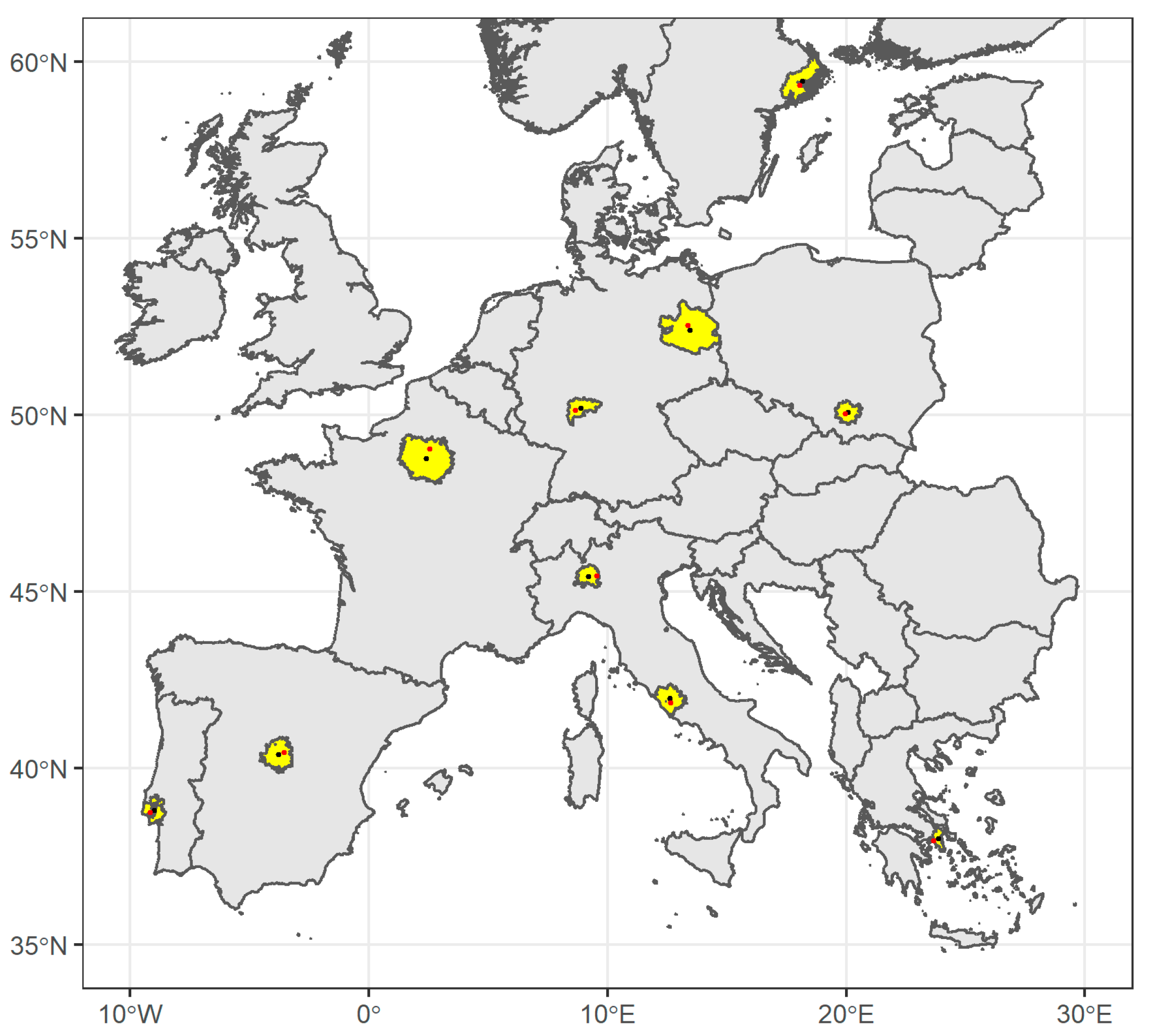
2.2. Selection of Cities and Simulations
- The ’baseline’ simulation (reference), considering the 2015 as reference year.
- The ’city scenario’: in which all the emissions from the 10 cities are switched off. As cities are far away from each other, we assume that impacts from other cities on the city of interest are negligible.
- The ’urban scenario’: in which emissions from all urban areas with a population > 300/km2 are switched off, in addition to the 10 cities themselves. This scenario allows for estimating the additional benefit of reducing urban emissions around each city.
- The ’agriculture scenario’: in which agricultural emissions are switched off, on top of the ’city’ and ’urban’ reductions. This is useful to evaluate the additional benefit on urban air quality of reducing one of the main emission sources in rural areas.
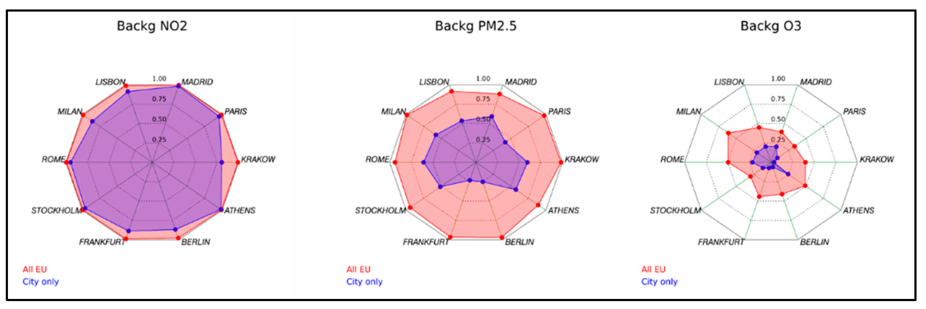
- The ’EU wide scenario’: in which all-anthropogenic emissions remaining in Europe (here intended as the modelling domain) are switched off. This simulation is intended to assess the additional benefit from EU wide actions (the background contribution is derived by the baseline concentration simulation, summing up the components related to sea salt and dust).
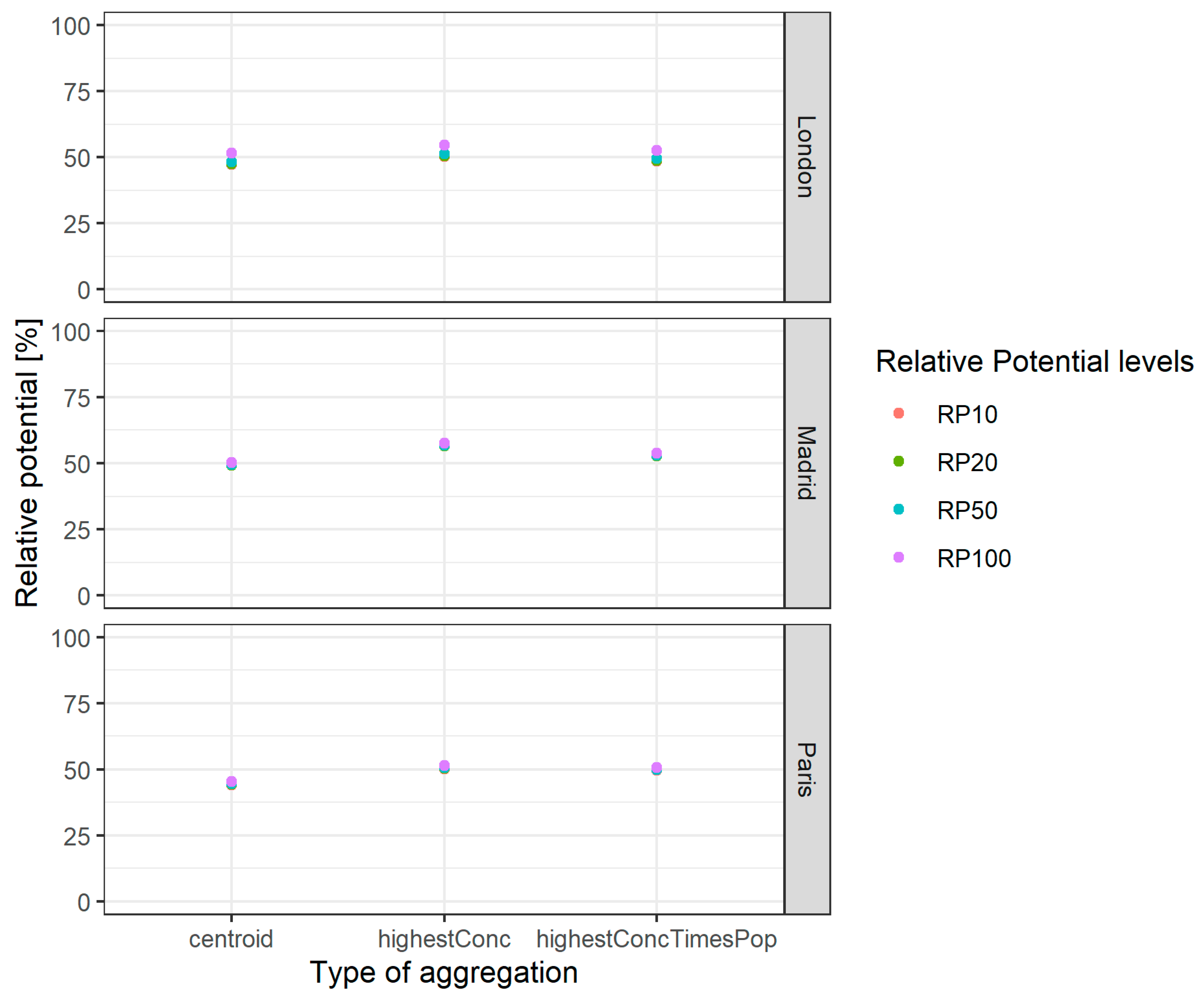
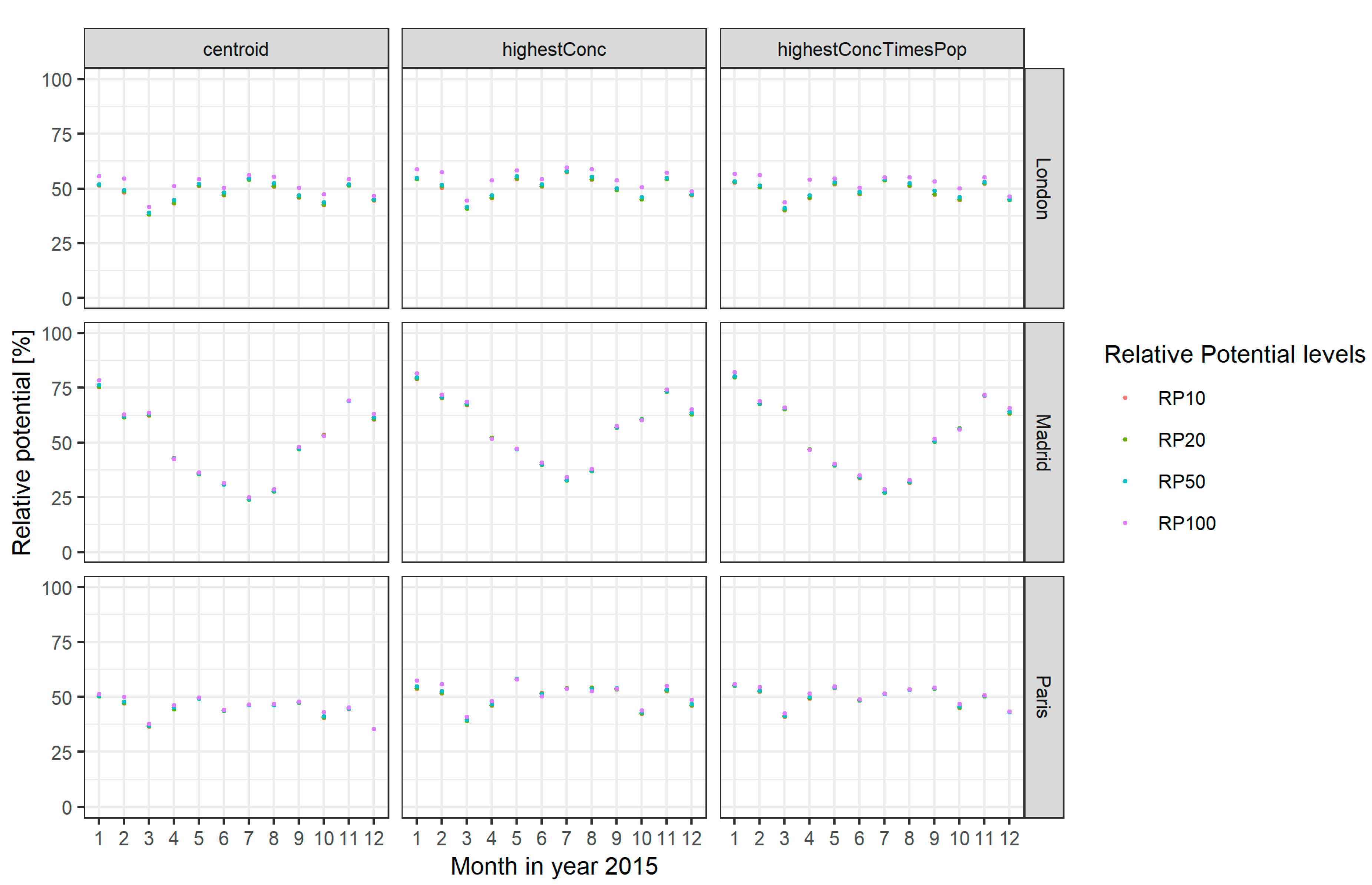
- The centroid of the city ‘functional urban area’;
- The location of the highest modelled concentration within the FUA (Functional Urban Areas [20]).
3. Results
3.1. Why a Focus on PM2.5
3.2. Contribution to PM2.5
3.2.1. Yearly Average Results
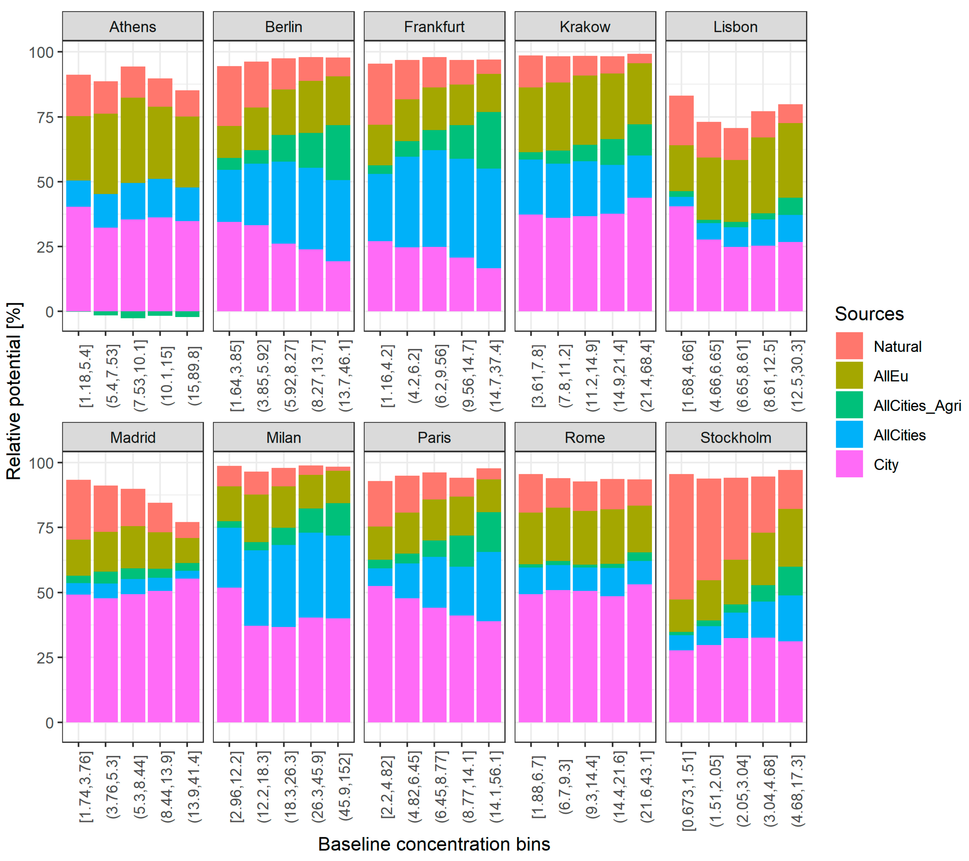
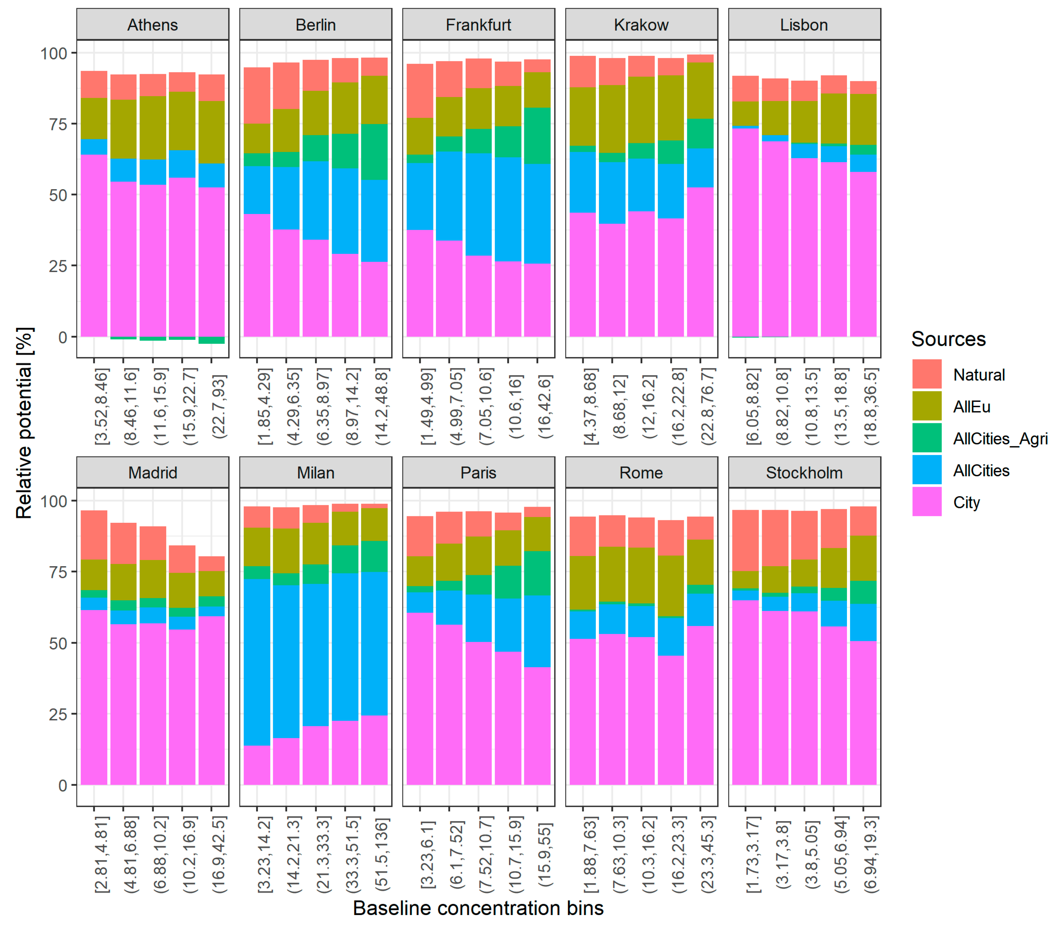
- City: represents the case reducing emissions in the 10 cities;
- AllCities: represents the case reducing all urban areas emissions;
- AllCities_Agri: represents the case reducing all urban areas emissions and agricultural emissions;
- AllEu: represents the case reducing all anthropogenic emissions;
- Natural: represent the remaining concentrations.
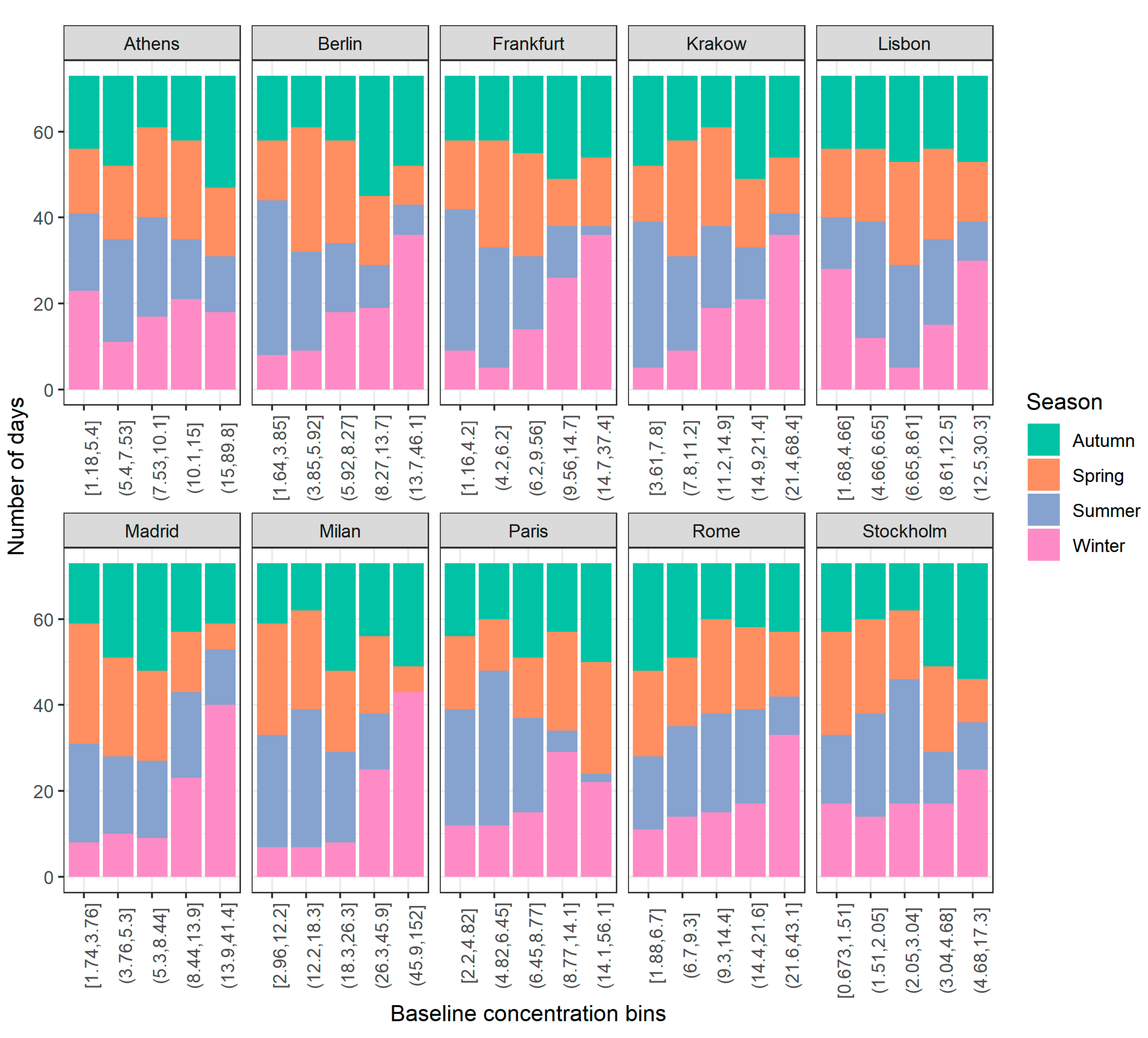
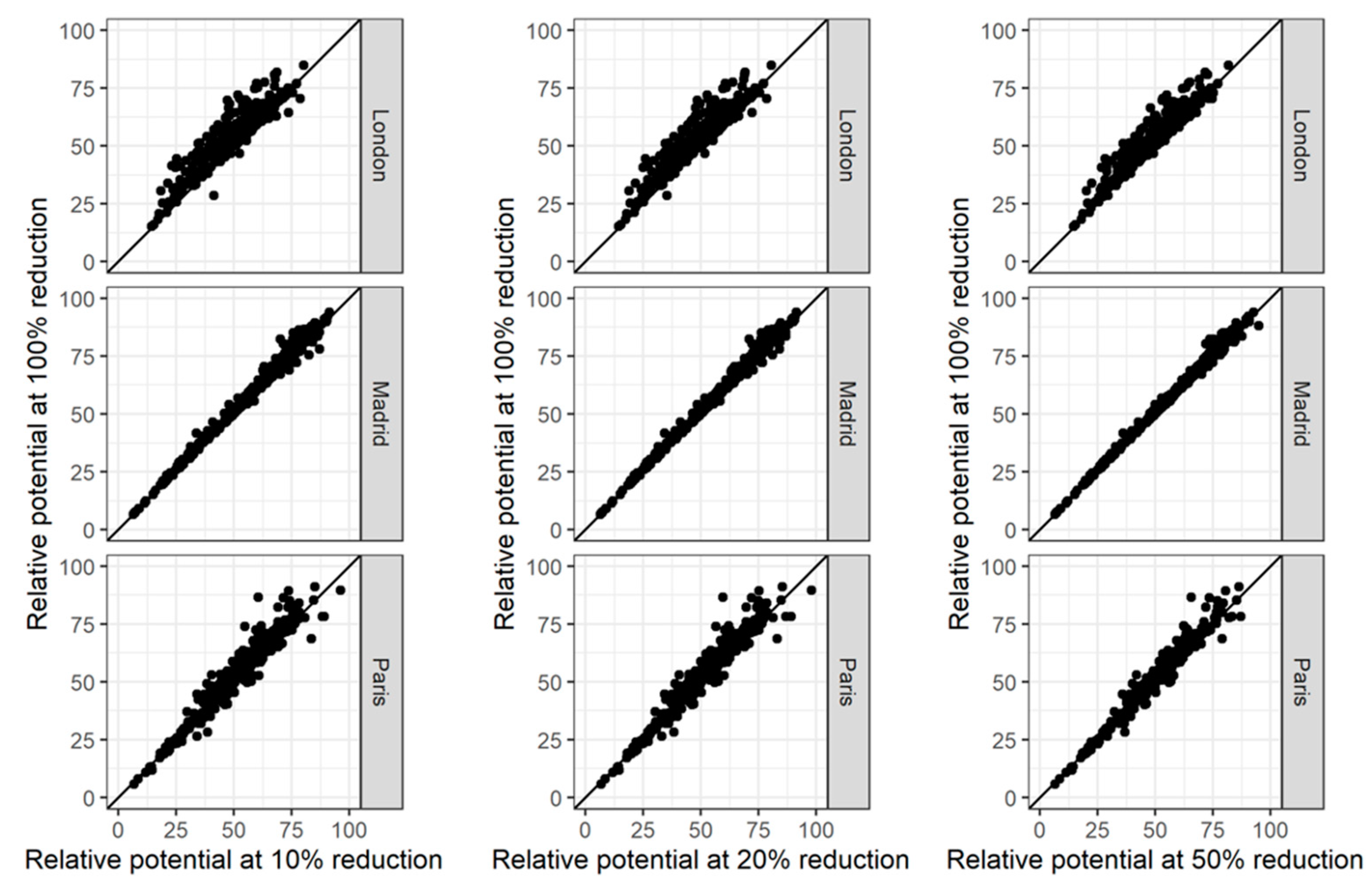
- Cities in which the ‘city’ impact gets less important when concentrations increase: Berlin, Frankfurt, Milan, Paris, Lisbon. For these cities, local plans are not sufficient to abate high pollution episodes;
- Cities in which the ‘city’ impact is independent of the concentration level: Athens, Rome and Stockholm. Local plans will have the same efficiency regardless of the concentration levels;
- Cities in which the ‘city’ impact becomes more important when concentration levels increase: Krakow and Madrid. Local plans are then more effective during high concentration episodes.
3.2.2. Yearly vs. Seasonal Results
3.2.3. Centroid vs. Hot-Spot Receptor
3.3. Nonlinearities and Temporal Trends Assessment
4. Conclusions
Supplementary Materials
Author Contributions
Funding
Data Availability Statement
Conflicts of Interest
References
- Kim, K.-H.; Kabir, E.; Kabir, S. A review on the human health impact of airborne particulate matter. Environ. Int. 2015, 74, 136–143. [Google Scholar] [CrossRef] [PubMed]
- Ohlwein, S.; Kappeler, R.; Kutlar Joss, M.; Künzli, N.; Hoffmann, B. Health effects of ultrafine particles: A systematic literature review update of epidemiological evidence. Int. J. Public Health 2019, 64, 547–559. [Google Scholar] [CrossRef] [PubMed]
- Shah, A.S.V.; Lee, K.K.; McAllister, D.A.; Hunter, A.; Nair, H.; Whiteley, W.; Langrish, J.P.; Newby, D.E.; Mills, N.L. Short term exposure to air pollution and stroke: Systematic review and meta-analysis. BMJ 2015, 350, h1295. [Google Scholar] [CrossRef] [PubMed] [Green Version]
- Lasry, F.; Coll, I.; Fayet, S.; Havre, M.; Vautard, R. Short-term measures for the control of ozone peaks: Expertise from CTM simulations. J. Atmos. Chem. 2007, 57, 107–134. [Google Scholar] [CrossRef]
- Pisoni, E.; Christidis, P.; Thunis, P.; Trombetti, M. Evaluating the impact of “Sustainable Urban Mobility Plans” on urban background air quality. J. Environ. Manag. 2019, 231, 249–255. [Google Scholar] [CrossRef]
- Pisoni, E.; Guerreiro, C.; Lopez-Aparicio, S.; Guevara, M.; Tarrason, L.; Janssen, S.; Thunis, P.; Pfäfflin, F.; Piersanti, A.; Briganti, G.; et al. Supporting the improvement of air quality management practices: The “FAIRMODE pilot” activity. J. Environ. Manag. 2019, 245, 122–130. [Google Scholar] [CrossRef]
- Thunis, P.; Clappier, A.; Tarrason, L.; Cuvelier, C.; Monteiro, A.; Pisoni, E.; Wesseling, J.; Belis, C.; Pirovano, G.; Janssen, S.; et al. Source apportionment to support air quality planning: Strengths and weaknesses of existing approaches. Environ. Int. 2019, 130, 104825. [Google Scholar] [CrossRef]
- Thunis, P.; Degraeuwe, B.; Pisoni, E.; Meleux, F.; Clappier, A. Analyzing the efficiency of short-term air quality plans in European cities, using the CHIMERE air quality model. Air Qual. Atmos. Health 2017, 10, 235–248. [Google Scholar] [CrossRef]
- Borge, R.; Santiago, J.L.; de la Paz, D.; Martín, F.; Domingo, J.; Valdés, C.; Sánchez, B.; Rivas, E.; Rozas, M.T.; Lázaro, S.; et al. Application of a short term air quality action plan in Madrid (Spain) under a high-pollution episode—Part II: Assessment from multi-scale modelling. Sci. Total Environ. 2018, 635, 1574–1584. [Google Scholar] [CrossRef]
- Akritidis, D.; Katragkou, E.; Zanis, P.; Pytharoulis, I.; Melas, D.; Flemming, J.; Inness, A.; Clark, H.; Plu, M.; Eskes, H. A deep stratosphere-to-troposphere ozone transport event over Europe simulated in CAMS global and regional forecast systems: Analysis and evaluation. Atmospheric Chem. Phys. 2018, 18, 15515–15534. [Google Scholar] [CrossRef] [Green Version]
- Marecal, V.; Peuch, V.-H.; Andersson, C.; Andersson, S.; Arteta, J.; Beekmann, M.; Benedictow, A.; Bergstrom, R.W.; Bessagnet, B.; Cansado, A.; et al. A regional air quality forecasting system over Europe: The MACC-II daily ensemble production. Geosci. Model Dev. 2015, 8, 2777–2813. [Google Scholar] [CrossRef] [Green Version]
- Adani, M.; Piersanti, A.; Ciancarella, L.; D’Isidoro, M.; Villani, M.G.; Vitali, L. Preliminary Tests on the Sensitivity of the FORAIR_IT Air Quality Forecasting System to Different Meteorological Drivers. Atmosphere 2020, 11, 574. [Google Scholar] [CrossRef]
- Singh, V.; Carnevale, C.; Finzi, G.; Pisoni, E.; Volta, M. A cokriging based approach to reconstruct air pollution maps, processing measurement station concentrations and deterministic model simulations. Environ. Model. Softw. 2011, 26, 778–786. [Google Scholar] [CrossRef]
- Agarwal, S.; Sharma, S.; Suresh, R.; Rahman, M.H.; Vranckx, S.; Maiheu, B.; Blyth, L.; Janssen, S.; Gargava, P.; Shukla, V.K.; et al. Air quality forecasting using artificial neural networks with real time dynamic error correction in highly polluted regions. Sci. Total Environ. 2020, 735, 139454. [Google Scholar] [CrossRef]
- Thunis, P.; Degraeuwe, B.; Pisoni, E.; Trombetti, M.; Peduzzi, E.; Belis, C.A.; Wilson, J.; Clappier, A.; Vignati, E. PM2.5 source allocation in European cities: A SHERPA modelling study. Atmos. Environ. 2018, 187, 93–106. [Google Scholar] [CrossRef]
- Simpson, D.; Benedictow, A.; Berge, H.; Bergström, R.; Emberson, L.D.; Fagerli, H.; Flechard, C.R.; Hayman, G.D.; Gauss, M.; Jonson, J.E.; et al. The EMEP MSC-W chemical transport model—Technical description. Atmos. Chem. Phys. 2012, 12, 7825–7865. [Google Scholar] [CrossRef] [Green Version]
- Granier, C.; Darras, S.; van der Gon, H.D.; Doubalova, J.; Elguindi, N.; Galle, B.; Gauss, M.; Guevara, M.; Jalkanen, J.-P.; Kuenen, J.; et al. The Copernicus Atmosphere Monitoring Service Global and Regional Emissions (April 2019 Version), Report April 2019 version; Copernicus Atmosphere Monitoring Service: Reading, UK, 2019. [Google Scholar] [CrossRef]
- Kuenen, J.; Dellaert, S.; Visschedijk, A.; Jalkanen, J.-P.; Super, I.; van der Gon, H.D. CAMS-REG-v4: A state-of-the-art high-resolution European emission inventory for air quality modelling. Earth Syst. Sci. Data 2022, 14, 491–515. [Google Scholar] [CrossRef]
- Thunis, P.; Crippa, M.; Cuvelier, C.; Guizzardi, D.; de Meij, A.; Oreggioni, G.; Pisoni, E. Sensitivity of air quality modelling to different emission inventories: A case study over Europe. Atmospheric Environ. X 2021, 10, 100111. [Google Scholar] [CrossRef]
- Dijkstra, L.; Poelman, H.; Veneri, P. The EU-OECD definition of a functional urban area. In OECD Regional Development Working Papers; No. 2019/11; OECD Publishing: Paris, France, 2019. [Google Scholar] [CrossRef]
- Itahashi, S.; Mathur, R.; Hogrefe, C.; Napelenok, S.L.; Zhang, Y. Modeling stratospheric intrusion and trans-Pacific transport on tropospheric ozone using hemispheric CMAQ during April 2010—Part 2: Examination of emission impacts based on the higher-order decoupled direct method. Atmospheric Chem. Phys. 2020, 20, 3397–3413. [Google Scholar] [CrossRef] [Green Version]
- Fiore, A.M.; West, J.J.; Horowitz, L.W.; Naik, V.; Schwarzkopf, M.D. Characterizing the tropospheric ozone response to methane emission controls and the benefits to climate and air quality. J. Geophys. Res. 2008, 113, 8307. [Google Scholar] [CrossRef] [Green Version]
- Derwent, R.G.; Utembe, S.R.; Jenkin, M.E.; Shallcross, D.E. Tropospheric ozone production regions and the intercontinental origins of surface ozone over Europe. Atmos. Environ. 2015, 112, 216–224. [Google Scholar] [CrossRef]
- Butler, T.; Lupascu, A.; Coates, J.; Zhu, S. TOAST 1.0: Tropospheric Ozone Attribution of Sources with Tagging for CESM 1.2.2. Geosci. Model Dev. 2018, 11, 2825–2840. [Google Scholar] [CrossRef] [Green Version]
- Bessagnet, B.; Beauchamp, M.; Guerreiro, C.; de Leeuw, F.; Tsyro, S.; Colette, A.; Meleux, F.; Rouïl, L.; Ruyssenaars, P.; Sauter, F.; et al. Can further mitigation of ammonia emissions reduce exceedances of particulate matter air quality standards? Environ. Sci. Policy 2014, 44, 149–163. [Google Scholar] [CrossRef]
- Thunis, P.; Clappier, A.; de Meij, A.; Pisoni, E.; Bessagnet, B.; Tarrason, L. Why is the city’s responsibility for its air pollution often underestimated? A focus on PM2.5. Atmos. Chem. Phys. 2021, 21, 18195–18212. [Google Scholar] [CrossRef]
- Thunis, P.; Clappier, A.; Pisoni, E.; Degraeuwe, B. Quantification of non-linearities as a function of time averaging in regional air quality modeling applications. Atmos. Environ. 2015, 103, 263–275. [Google Scholar] [CrossRef]
Publisher’s Note: MDPI stays neutral with regard to jurisdictional claims in published maps and institutional affiliations. |
© 2022 by the authors. Licensee MDPI, Basel, Switzerland. This article is an open access article distributed under the terms and conditions of the Creative Commons Attribution (CC BY) license (https://creativecommons.org/licenses/by/4.0/).
Share and Cite
Pisoni, E.; Thunis, P.; De Meij, A.; Bessagnet, B. Assessing the Impact of Local Policies on PM2.5 Concentration Levels: Application to 10 European Cities. Sustainability 2022, 14, 6384. https://doi.org/10.3390/su14116384
Pisoni E, Thunis P, De Meij A, Bessagnet B. Assessing the Impact of Local Policies on PM2.5 Concentration Levels: Application to 10 European Cities. Sustainability. 2022; 14(11):6384. https://doi.org/10.3390/su14116384
Chicago/Turabian StylePisoni, Enrico, Philippe Thunis, Alexander De Meij, and Bertrand Bessagnet. 2022. "Assessing the Impact of Local Policies on PM2.5 Concentration Levels: Application to 10 European Cities" Sustainability 14, no. 11: 6384. https://doi.org/10.3390/su14116384
APA StylePisoni, E., Thunis, P., De Meij, A., & Bessagnet, B. (2022). Assessing the Impact of Local Policies on PM2.5 Concentration Levels: Application to 10 European Cities. Sustainability, 14(11), 6384. https://doi.org/10.3390/su14116384


