Risk Levels Classification of Near-Crashes in Naturalistic Driving Data

Abstract

Identifying dangerous events from driving behavior data has become a vital challenge in intelligent transportation systems. In this study, we compared machine and deep learning-based methods for classifying the risk levels of near-crashes. A dataset was built for the study by considering variables related to naturalistic driving, temporal data, participants, and road geometry, among others. Hierarchical clustering was applied to categorize the near-crashes into several risk levels based on high-risk driving variables. The adaptive lasso variable model was adopted to reduce factors and select significant driving risk factors. In addition, several machine and deep learning models were used to compare near-crash classification performance by training the models and examining the model with testing data. The results showed that the deep learning models outperformed the machine learning and statistical models in terms of classification performance. The LSTM model achieved the highest performance in terms of all evaluation metrics compared with the state-of-the-art models (accuracy = 96%, recall = 0.93, precision = 0.88, and F1-measure = 0.91). The LSTM model can improve the classification accuracy and prediction of most near-crash events and reduce false near-crash classification. The finding of this study can benefit transportation safety in predicting and classifying driving risk. It can provide useful suggestions for reducing the incidence of critical events and forward road crashes.

1. Introduction

As a result of the considerable increase of motor vehicles, traffic crashes have become one of the most serious and threatening challenges that significantly influence people and society and result in economic losses, injuries, and fatalities. According to World Health Organization (WHO) [1], every year more than 1.2 million people lose their lives in road crashes. In addition, 20–50 million people suffer non-fatal injuries or become disabled as a result of their injury. Due to these increasing numbers, traffic safety-related issues have received considerable research attention [2,3,4,5]. Although various approaches have explored driving behaviors for avoiding and reducing road crashes, key questions remain: how can driving performance be effectively evaluated, and how can driving risk be predicted and classified by the information acquired from the driver, vehicle, weather, and road geometry scheme [6,7]. Driving risk analysis is still challenging [8] for a number of reasons.

Firstly, crash severity-related datasets regarding quality and quantity are lacking. Secondly, there is a need to provide an effective method to select the significant variables of driving risk before conducting crash severity analysis. Thirdly, in studies on crash risk prediction and classification, a method that analyzes the high risk levels of driving variables and classifies driving events is needed, and a validation process needs to be included. To the best of the authors’ knowledge, these problems are still neglected in road safety-related studies. There is a need to compare predictive performance using statistical, machine, and deep learning methods.

Through this study, we explore the significant variables associated with near-crash events using a multi-source dataset. Near-crash events are identified by exploring significant driving behavior actions. Subsequently, near-crashes are classified and grouped into several levels according to their driving risk parameters. As there are many variables in the collected data, we adopted the selection feature method to choose only significant variables for near-crash events. Many classification models of statistical, machine, and deep learning are applied for near-crash classification. To sum up, the main contributions of this paper are concluded as follows: (1) Hierarchical clustering is adopted to group the near-crashes based on high-risk driving features. (2) Adaptive lasso regression is utilized to select significant variables related to high driving risks. (3) Various classification models are applied on near-crash data to predict and classify their risk levels. Seven machine, deep, and statistical models are trained and tested using the near-crash dataset, and evaluation metrics validate the performance of the classification models in terms of accuracy and running time.

The remainder of the paper is organized as follows. Section 2 introduces the related work. A description of the proposed methodology is presented in Section 3. The results of the experiments are provided in Section 4. A discussion of the results and a comparison with other related classification approaches are presented in detail in Section 5, and the study conclusions are finally discussed, along with the value of the findings and future work.

2. Related Work

In recent decades, many approaches have been taken to analyze and understand crash injury severity.

In general, the most popular methods used for road crash-related analysis are statistical models. For instance, ordinal logistic regression and multinomial regression are adopted to explore the important variables for severe truck and vehicle crashes. Their result showed that factors such as being a non-resident, driving in off-peak hours, and driving on weekends may increase the risk of truck crashes [2]. Wang et al. [3] used a CART classification model to investigate the correlations among driving behavior, vehicle attributes, road geometry condition, and driver characteristics. Naji et al. [4] used a mixed-ordered regression model to evaluate the dangerous levels using near-crash events. Their findings showed that many variables influence driving risk, including the deceleration average, road congestion, the road type, the time of day, and the driver’s mileage, experience, and age.

Although statistical models have been largely utilized for crash prediction and classification, these models suffer from poor data quality, require knowledge of data distributions in advance, and require a large amount of data. Therefore, machine learning (ML)-based models, such as support vector machines (SVMs), the K-nearest neighbor (KNN), and random forests (RFs), have been adopted and have achieved better results in many transportation systems [5,7]. Duong [8] adopted a multilayer perceptron (MLP) for a binary classification of crash fatalities. An SVM was applied to investigate the injury severity factors of zone crashes [9]. Princess et al. [10] adopted the k-nearest neighbor and support vector machine to classify the severity of road accidents. Jie Xie and Mingying Zhu [11] utilized a random forest for classifying maneuver-based driving behaviors and analyzing aggressive driving.

Mokhtarimousavi [12] analyzed naturalistic diving data by extreme gradient boosting (in short, XGBoost) and AdaBoost to determine the significant factors of near-crashes. Wang et al. [13] utilized machine learning methods to analyze and predict driving risk and found that artificial neural networks (ANNs) achieved better performance results compared to other methods. Many other studies [14,15,16] compared various ML methods for crash risk classifications and prediction and achieved perfect results.

With the rapid advance and increase in new methods in deep learning, these models have proved to be reliable tools for crash risk analysis [17]. Li et al. [18] introduced a real-time crash risk prediction approach by merging long short-term memory (LSTM) and a convolutional neural network (CNN). Another approach proposed for analyzing real-time crash risk is to consider time series dependency using an LSTM model [19]. Jiang et al. [20] adopted LSTM networks for crash identification based on freeway traffic data. In [21], a convolutional neural network (CNN) approach with refined loss functions was adopted to analyze crash risk severity. Zhao et al. [22] proposed a convolutional neural network with gated convolutional layers (G-CNN) to analyze crash risk in each traffic state.

However, there is a need to explore driving behavior analysis using near-crash events to classify and predict driving risk levels. Moreover, for investigating the correlation between high-risk driving and behavior variables, there is a need to provide an efficient and effective variable selection method of choosing significant variables related to high-risk driving. Hierarchical clustering has been applied to categorize near-crashes into several risk levels according to driving behavior to address these issues. In addition, adaptive lasso regression has been adopted for variable selection, which reduces the data dimensions and time complexity.

With the recent advance in data collection, many researchers have begun considering using naturalistic driving data to investigate and analyze high-risk driving. For instance, NHTSA presented the “100-Car Naturalistic Driving Study” project to obtain naturalistic driving data. [23]. With the availability of such data, traffic safety researchers have developed new methods to better explore the risk levels associated with the driving behavior of individual drivers.

As traffic crash data are scarce and not always available [24,25], naturalistic driving studies have become one of the best methods for collecting driving behavior data and presenting near-crashes as surrogate measures. Osman et al. [26] compared several machine learning models for predicting near-crashes from observed vehicle kinematic variables. Seacrist et al. [27] utilized naturalistic driving data to compare and analyze the frequency and characteristics of a high-risk driver’s near-crashes. Naji et al. [4,28] adopted two logit regression models to explore the affecting factors of driving risk on near-crashes and individual drivers. Perez adopted a method for identifying and validating near-crash events using different kinematic thresholds [29]. In [30], the authors proposed an approach for investigating the involvement of secondary tasks in near-crashes to study the impact of driving behavior factors on traffic safety.

However, the driving data collected by naturalistic driving experiments may not be enough to understand the driving risk patterns; therefore, other data sources can enrich the driving data and add more significant variables correlated to crash analysis. In addition to the obtained variables from naturalistic driving data, we considered various variables from driver input, geometry, time, and weather data in this study.

Regarding near-crash analysis, we found that no comprehensive study considers near-crash analysis via statistical, machine, and deep learning models for classifying and predicting high-risk levels. In addition, to the best of the authors’ knowledge, there is still limited research comparing the classification performance of various statistical, ML, and DL models with a detailed validation.

To sum up, the main goal of this study was to use the collected data from a naturalistic driving study (NDS) along with related datasets for classifying and predicting the dangerous levels of near-crash events. Our study utilized hierarchical clustering to group near-crashes into risk levels using driving behavior variables. Adaptive lasso regression was applied to filter the collected variables, considering significant variables only. In addition, seven statistical, machine, and deep learning models were adopted to classify the risk levels of near-crashes. The classifier models were trained with training data and validated with testing data. Finally, the classifier’s performance was compared and validated by evaluation metrics, including accuracy, recall, precision, and F1-measure.

3. Methodology

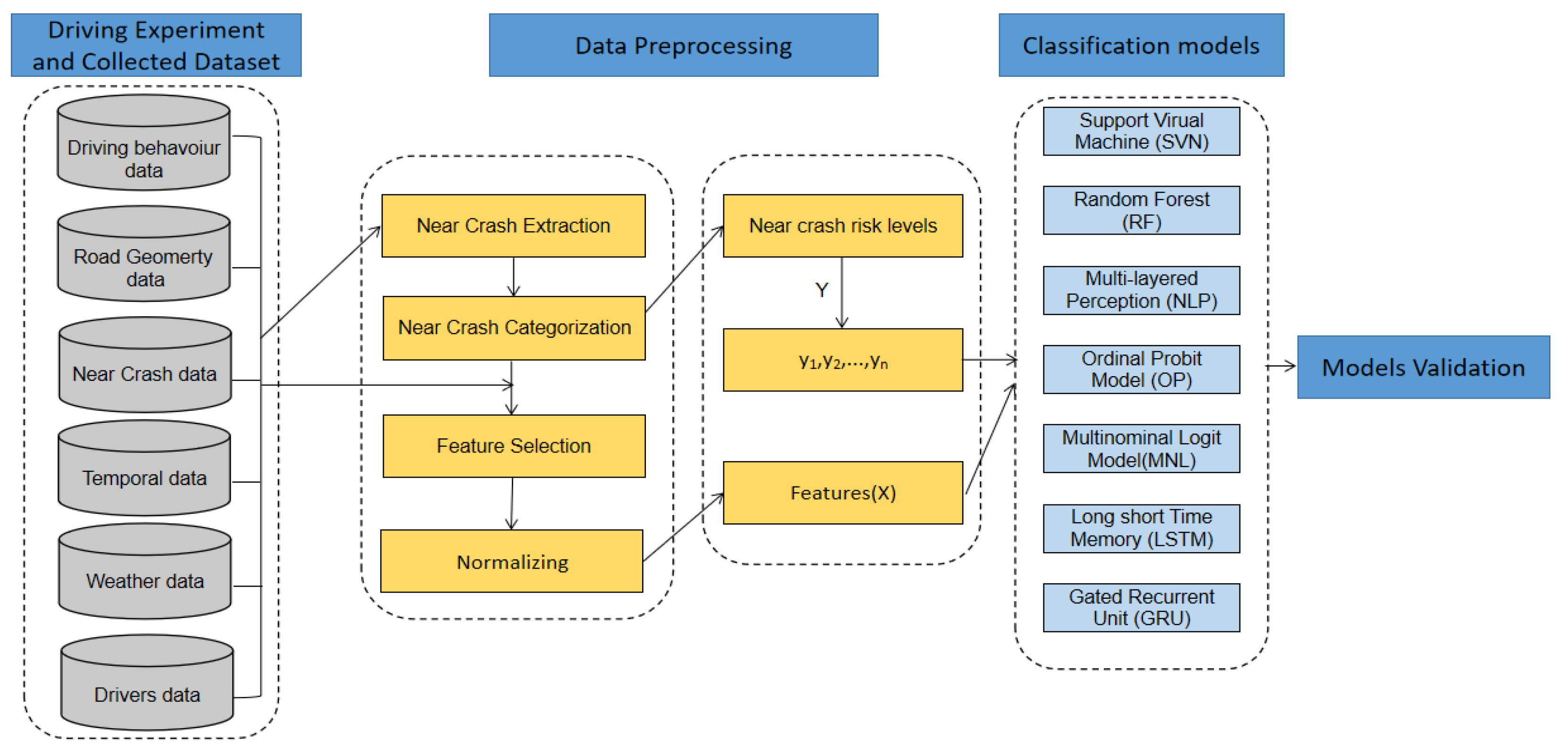
This section introduces the proposed model for classifying driving risk of near-crash events in detail, including the driving experiment and collected dataset, data preprocessing, classification models, and validation. Figure 1 depicts the framework of the proposed model.

3.1. The Driving Experiment and Collected Dataset

For classifying the driving risk levels of near-crashes, we needed to collect a robust and suitable dataset. Here, we explain the experiment and collected data in detail.

Naturalistic driving experiments were performed via a carefully prepared vehicle driven on various road types in Wuhan, China. An experimental vehicle was equipped with various devices such as CAN BUS, MobilEye, LiDAR, and a video camera. These devices can synchronously collect vehicle speed, acceleration-related variables, braking signals, time headway, vehicle position, and road condition. Forty-one drivers joined the experiment, including 11 female and 30 male drivers. Their age ranged between 18 and 56 years with various educational backgrounds. Regarding the driving experience, all participants had driving experience from 2 years to more than 10 years. For the sake of investigating the impact of road types on driving behavior, an experimental route was planned to include all road types. Figure 2 shows the experimental route on the roads of the city of Wuhan.

The experiment route’s length was 90 km, and the ordinary driving period was 90 min. As shown in Figure 2, the route was composed of four segments, namely an expressway, a freeway, an expressway, and an urban road. The expressway segment had a 10 km length and an 80 km/h speed limit. The freeway segment had a permitted speed of 100–120 km/h, and the length was 38 km. The speed limit of the urban expressway segment was 80 km/h, and the length was 31 km. The urban road segment had a permitted speed of 40–60 km/h and the shortest length of 12 km.

In addition, experiments performed at different day times ranged from 8:00 to 20:00 and on different weather conditions. To sum up, all variables in the collected dataset are listed in

Table 1. Variables of the collected dataset.

Variable	Symbol	Type	Details
Driving Behavior (Vehicle Status)
Beginning Speed	Begin_Sp	continuous	Vehicle velocity once a near-crash happens (m/s)
Average of Deceleration	Avg_Dec	continuous	Average of Deceleration (m/s2)
Average of Speed	Avg_Sp	continuous	Average of Speed (m/s)
Time Headway Average	Avr_THW	continuous	Average of Time Headway(s)
Braking Pressure Average	Avr_Br	continuous	Average of Braking Pressure(MPA)
Minimum Deceleration	Min_Dec	continuous	Minimum Deceleration(m/s2)
Minimum Time Headway	MinTHW	continuous	Minimum Time Headway(s)
Max Braking Pressure	Max_Br	continuous	Maximum Braking Pressure (mpa)
Kinetic Energy	Eneg	continuous	Vehicle Kinetic Energy
Road Condition
Wet	Wet	nominal	1. Wet 2. Dry
Road Type	R_ty	nominal	1. Expressway 2. Freeway 3. Urban Expressway 4. Urban road.
Lane Numbers	Lane_Nu	nominal	1. 1; 2.2; 3.3; 4.4; 5.5
Speed Limit	Sp_lim	nominal	1. 40–60; 2.80; 3.100–120
Road Congestion	congested	nominal	1. Yes; 0. No
Weather	Weather	nominal	1. Sunny; 2. Rain; 3. Cloud
Light	Light	nominal	1. Light; 2.Dark
Time Variables
Peak Hour	Peak_hrs	nominal	1. Yes; 2. No
Weekend	Weekend	nominal	1. Yes; 2. No
Time of Day	Time_day	nominal	1. 6:00–12:00; 2. 12:00:−18:00; 3. 18:00–24:00
Driver Inputs
Education Level	Edu_lev	nominal	1. Less than graduate 2. graduate 3. Post-graduate and above
Age	Age	nominal	1. less than 23; 2. 23–45; 3. More than 45
Gender	Gender	categorical	1. Male 2. Female
Driving Miles	Dri_ miles	continues	Driving Miles (miles)
Driving Experience	Dri_years	continuous	Driving license (years)

.

3.2. Data Preprocessing

3.2.1. Near-Crash Extraction

As near-crashes are not found among police-reported data nor included in archival databases, the naturalistic driving study (NDS) became a popular method for studying them [31]. In [32], researchers considered braking events as near-crash events. A near-crash was considered once the acceleration reached certain values (lateral: −1 m/s², longitudinal: −1.5 m/s²) [33]. Our study defined a near-crash by exploring three significant driving variables, including deceleration, braking pressure, and time headway, as in [4,34]. In naturalistic driving experiments, a near-crash can be detected by achieving at least one of the following three thresholds of driving variables: an acceleration under −0.4 m/s², a time headway below 0.6 s, or a braking pressure above 10 mph. In addition, the collected near-crashes were validated by checking the recorded videos on the related timestamps to find whether a near-crash occurred or not. Finally, several near-crash-related variables can be appended to the variables in Section 3.1.

Table 2. Variables related to near-crash events.

Factor	Symbol	Type	Details
Near-Crash Type	NC_type	nominal	1. Subject-Vehicle (Head) vs. Object-Vehicle (Head) 2. Subject-Vehicle (Head) vs. Object-Vehicle (Tail) 3. Subject-Vehicle (Head) vs. Object-Vehicle (Side) 4. Subject-Vehicle (Side) vs. Object-Vehicle (Side) 5. Subject-Vehicle (Side) vs. Object-Vehicle (Tail) 6. Conflict with Pedestrian 7. Parts of Road 8. Others
Near-Crash Reason	NC_reason	nominal	1. Head-vehicle abruptly halted 2. Traffic Signals 3. Traffic Jam 4. Road Repairs 5. Road changes 6. Pedestrians 7. Subject-Vehicle turned-off 8. Object-Vehicle turned-off 9. Others

illustrates these variables in detail.

3.2.2. Near-Crash Categorization

Various statistical and data analysis approaches have been adopted for traffic safety to understand the daily driving behavior and patterns. Among these methods, cluster analysis has been adopted to group driving data into several categories [35,36]. K-means, hierarchical clustering, and DBSCAN are prevalent methods applied in traffic safety analysis.

Hierarchical clustering (HC) is commonly used for similar grouping objects into multiple-level hierarchical clusters. For implementing hierarchical clustering, two methods can be adopted: the agglomerative method and the divisive method. N-1 levels (clusters) are built as a result of the HC model [37].

In our study, hierarchical clustering was applied to categorize near-crashes into clusters by considering related driving risk variables (acceleration, time headway, and braking pressure), which resulted in a hierarchical clustering dendrogram. With the agglomerative method, the process began with zero clusters, and each near-crash event was then considered a core cluster. Subsequently, two highly similar clusters were combined as a new cluster, and the algorithm terminated once all near-crashes formed a single cluster. A distance measure was used to determine the correlation between events via calculating the similarity between near-crashes and visually represented by points in the clustering dendrogram. The Euclidean distance [37] is the most prevalent method used in hierarchical clustering. The distance of two near-crashes was calculated using Equation (1).

$${\mathrm{dist}}_{\mathrm{Euclidean}}\left(x,y\right)=\sqrt{{{\displaystyle \sum }}_{i=1}^p{\left(x_i-y_i\right)}^2}$$

(1)

where x and y are near-crashes, and p is the total of near-crashes.

The hierarchical clustering generated several categories presenting the risk levels of near-crash events.

3.2.3. Feature Selection

The dimensionality reduction of input variables through the feature selection method before applying classification models is vital. In other words, removing redundant dimensions decreases training time significantly without affecting the models’ performance.

As naturalistic experiments can collect various variables, there is a need to explore the relationships between key factors and the outcome variable(s). More specifically, it becomes a challenge to optimally identify and use only variables that are relevant to the outcome to provide us with useful information. Many methods have been utilized to address this issue; however, this problem can be more complicated when the factors and the outcome have a non-linear correlation. Therefore, we adopted adaptive lasso regression to perform variable selection when analyzing non-linear relationships [38]. Assume we have the given n independent observations (X_i, y_i), i = 1, 2, …, n, which are generated as follows:

$$y_i=\mathrm{g}\left(X_i^{T}w\right)+{\epsilon }_i, i=1, 2, \dots , n$$

(2)

where ${\epsilon }_i$ is a Gaussian random variable, ${\epsilon }_i$~n$\in$ (0, σ²), function g: R → R denotes a non-linear mapping function, which is not known a priori, and X_i ∈ R_p are feature vectors.

The main idea in the lasso method is to reduce the features in vectors by compassing a coefficient to zero and then setting a regression coefficient to zero, which lets us select optimal features. The model selection of the lasso method is essentially a process of seeking sparse model expressions, and this process can be completed by optimizing a function of “loss” and “penalty”. Lasso parameter estimation can be defined as Equation (3) [39]:

$$\stackrel{\wedge }{\beta } (\mathrm{lasso})=\arg \underset{\beta }{{min}^2}||y-{\displaystyle \sum }_{j=1}^m{x}_j{\beta }_j|{|}^2+\lambda {\displaystyle \sum }_{j=1}^m|{\beta }_j|$$

(3)

where $\lambda$ is a non-negative regular parameter, which controls the complexity of the model. The larger the value of $\lambda$, the greater the penalty for the linear model with more features. Finally, a model with fewer features is $\lambda {{\displaystyle \sum }}_{j=1}^m\left|{\beta }_j\right|$ obtained, which is the penalty term.

The $\lambda$ parameters can be determined using a cross-validation method, and the smallest error of $\lambda$ is obtained. Finally, according to the obtained values, the model is refit with all of the data.

3.2.4. Normalization

With various values of continuous variables, these variables are normalized to be between 0 and 1. This ensures that all factors can be treated equally during the training process for the classification models. To normalize the variables, the following equation is used:

$$x_{norm}=\frac{x-x_{mean}}{x_{min max}}$$

(4)

where x, x_min, x_max, and x_norm are the original, minimum, maximum, and normalized values from the dataset (training dataset), respectively.

3.3. Classification Models

This study applies two statistical models, three machine learning models, and two deep learning models for classification problems. These models have supervised learning methods that consider modeling the near-crashes’ risk levels Y (generated by hierarchical clustering method) and the input vector X as a classification problem. A support vector machine, a multi-layer perceptron, and a random forest were selected as machine learning models to implement the classification models. For deep learning, we chose an LSTM model and a gated recursive unit model. An ordinal probit model and a multinominal logit model were selected as statistical models.

3.3.1. Support Vector Machine (SVM)

The SVM method can map the input vector X into a high-dimensional variable space. The SVM designs an optimal separating hyper-plane in the dimensional space to separate the points that represent the vector X into groups while enlarging the margin among the linear decision boundaries. Therefore, SVM can be used to address classification problems. In an SVM model, the inputs are represented as vectors X_i∈R_n, for i = 1, 2,…, n, which denote a set of near-crash-related variables, and the output is defined as yi∈Rn, which represents the risk levels of the near-crashes. In addition, the hyper-plane for outputs could be drawn as a set of points X following Equation (5).

W × X − b = 0

(5)

where × represents the product process, W is a normal vector, and b is related to the predefined hyper-plane. In the SVM model, given a training set of instance-label pairs (X_i, y_i), by using the model, it needs to address the optimization problem [40] as follows:

$$\underset{w,b,\xi }{min}\frac{1}{2}{w}^{T}w+C{\displaystyle \sum }_{i=1}^N{\xi }_i$$

(6)

subject to

$$y_i\left(w^T\phi \left(x_i\right)+b\right)\ge 1-{\xi }_i, {\xi }_i\ge 0$$

(7)

where ξ are the parameters used to measure the misclassification errors, and C is a penalty parameter for errors as an additional capacity control by the classifier.

3.3.2. Random Forest (RF)

A random forest is a popular machine learning method for addressing classification, prediction, and other issues. The RF method generates many classifications and aggregates their results [41]. For solving a classification problem, the RF builds a multitude of decision trees at the training phase and outputs the level (class), which is the group of the levels (classes). Each node is split through the best in an RF among a subset of predictors randomly chosen at that specific node. Two hyper-parameters must be set in the RF model: the number of trees to grow and the number of variables randomly sampled as candidates at each split; by determining these parameters, RF can enhance the classification results [41].

3.3.3. Multi-Layer Perception (MLP)

The multi-layer perceptron is a type of artificial neural network (ANN). The MLP algorithm was selected to enhance the classification prediction performance. Artificial neural networks are considered efficient and applicable for predicting the correlation between the dependent and independent parameters. As in ANNs, MLPs’ prediction performance is highly affected by their inner structure, which contains an input layer, hidden layers, and an output layer. Each layer includes a group of neurons. Neurons are connected to others, transmit data from the last neuron, and multiply it by a specific weight based on the information strength in determining the output [42]. To train an MLP network, a forward and backward propagation method is repeatedly adopted to update all network weights. The outputs of an MLP model rely on connection weights, bias value, and activation function. The outputs can be calculated as follows:

$$y_i=f({\displaystyle \sum }_{j=0}^m{w}_{ij}{X}_i+b)$$

(8)

where f is an activation function, w denotes a weight value, X is an input vector, b and denotes the bias value.

3.3.4. Ordinal Probit Model (OP)

The ordinal probit model has been widely utilized for ordinal response data. If Y is a near-crash risk level, then a latent variable Y* is obtained, as in Equation (9) [2,43]:

Y* = X_i · β_i + ε_i

(9)

where Y* is a linear-based function that deals with discrete outcome, X_i is a vector of input variables, b is a vector of regression coefficients, and ε_i is an error that follows a logistic distribution with a mean of zero and a variance of ${\pi }^2/3$.

The risk level index will be transformed into a number set (1, 2,..., n) to be the outputs of the OP model, and the values of β and Y* can be calculated by the maximum likelihood estimation method [44].

3.3.5. Multinominal Logit Model (MNL)

The idea of a multinominal model is similar to an ordinal probit model. The main difference is that a multinominal model ignores the ordinal nature of outcomes. In other words, an MNL model can be used to deal with nominal outcomes [45]. The MNL model is presented as Equation (12):

$$P_i=\frac{e^{{\beta }_i{X}_i}}{{{\displaystyle \sum }}_i^N{e}^{{\beta }_i{X}_i}},i=1,2,\dots ,N$$

(10)

where P_i is the probability of a near-crash, which is labeled with the risk level (output) i, $\beta$_i is a vector of the calculative coefficient for the output risk level i, and X_i is an input vector. $\beta$_i coefficients can be calculated by the maximum likelihood approach.

3.3.6. Long-Short-Term Memory (LSTM)

In recent advances in deep learning methods, recurrent neural networks (RNNs) became one of the most successful approaches to applied classification problems [46]. LSTM neural networks are developed by adding a long-term memory function, which enhanced the RNNs’ ability to enhance the performance of classification and prediction. In a simple LSTM network, each feature vector X is mapped to a corresponding output vector y. Figure 3 depicts the structure of a simple LSTM unit.

An LSTM unit is composed of three layers, namely, an input layer, output layer, and memory block layer. The memory block layer contains three types of gates, including the input gate, the output gate ot, and the forget gate f_t. The calculation process in these layers during training are performed as follows [47]:

$$\begin{gathered} f_t=\sigma (W_f[h_{t-1},{\left\{X\right\}}_t]+b_f) \\ {i}_t=\sigma (W_i[h_{t-1},{\left\{X\right\}}_t]+b_i) \\ {o}_t=\sigma (W_o[h_{t-1},{\left\{X\right\}}_t]+b_o) \\ \sigma \left(x\right)=\frac{1}{1+exp(-x)} \end{gathered}$$

(11)

where t represents a random time step. $\sigma (.)$ is a sigmoid function, W_i, W_f, and Wc denote the weight of the input gate, the forget gate, and the output gate, respectively, In addition, the memory cell vectors ct and the candidate value $\widetilde{c_t}$ are calculated as follows:

$$\begin{gathered} \tilde{c}=\tan h(W_c[h_{t-1},{\left\{X\right\}}_t]+b_c) \\ {c}_t=f_t\times c_{t-1}+i_t\times {\tilde{c}}_t \\ {h}_t=o_t\times \tan h(c_t) \\ \tan h(x)=\frac{exp(x)-exp(-x)}{exp(x)+exp(-x)} \end{gathered}$$

(12)

During the training process of the LSTM model, the softmax function is utilized as the loss function, and the Adam optimizer method is adopted in the training process [47].

3.3.7. Gated Recursive Unit (GRU)

To reduce the training time of the LSTM model, the GRU model is developed. GRU is an RNN framework with a gate mechanism inspired by LSTM and a simpler structure [48]. The GRU architecture is shown in Figure 4.

A GRU cell contains update gate z_t and reset gate r_t. The reset gate (rt) utilizes the sigmoid function to properly reset the previous information and multiplies the value by the past hidden layer. The update gate (zt) is a combination of the forget and input gates as in the LSTM model. The update gate determines the rate of the update of the current and previous information. In the update gate, the result of the output as sigmoid determines the amount of information at the current node and the value subtracted from 1 (1 − z_t) is multiplied by the information of the hidden layer at the most recent time. Each update gate is similar to the input and forget gates of the LSTM. The output value can be obtained by multiplying the hidden layer’s value at the previous unit and the information at the present unit by weight with the following equations [49]:

$$\begin{gathered} z_t=\sigma (W_z{X}_t+U_z{h}_{t-1}) \\ {r}_t=\sigma (W_r{X}_r+U_r{h}_{r-1}) \\ {H}_t=\tan h\left(W_H{X}_t+U_{Hr}\left(r_t{h}_{t-1}\right)\right) \\ {h}_t=\left(1-z_t\right)h_{t-1}+z_t{H}_t \end{gathered}$$

(13)

where X_t is the input vector at time t, and W_z, U_z, W_r, U_r, W_H, U_H are the weight matrices for the nodes in GRU. Other information are similar to the information in LSTM.

4. Models Comparison and Results

To validate the performance of the utilized models, the classification models needed to be evaluated. In this section, first, we describe the experimental settings and the hyper-parameters of the classification models, followed by a description of the evaluation metrics. Finally, the obtained results are provided in detail.

4.1. Experimental Settings

The experiment was prepared and conducted as follows. Firstly, the near-crash dataset was divided into two parts, training (80%) and testing (20%). Secondly, the proposed models were trained based on the training dataset. At the end, the trained model was evaluated using the testing data.

We considered the impact of the hyper-parameters on the models’ performance; therefore, after manually training the adopted models, we found that the selected hyper-parameters resulted in improved classification.

Table 3. Hyper-parameters for classification models.

SVM	RF	MLP	LSTM	GRU
Penalty = 0.25	Max depth = 20, Estimators = 30 lass_weight: ‘balanced’, decision:entropy	hidden_layers = 4, epochs = 50, batch_size = 256	learning rate 0.0012, LSTM Unit Number = 16, hidden_layers:50, units:100, epochs: 100, batch_size: 512	Hidden layer = 20, learning rate = 0.001, epochs 100, batch_size: 512

shows the values of the hyper-parameters.

The classification models were implemented on a DELL PC, with a hardware environment of two GPUs and an NVIDIA GeForce RTX 2070 with a 32 GB memory and equipped with a 500 GB SSD drive, and were executed by codes written in R and Python. Machine and deep learning methods were implemented using the coding libraries of the scikit-learn and TensorFlow framework.

4.2. Evaluation Metrics

The performance of classifiers was examined by calculating the accuracy, recall, precision, F-measure, and their averages using the following equations [48]:

$$\begin{gathered} Accurac{y}_k=\frac{{\mathrm{TP}}_k+{\mathrm{TN}}_k}{{\mathrm{TP}}_k{+\mathrm{TN}}_k{+\mathrm{FP}}_k{+\mathrm{FN}}_k} \\ Accurac{y}_{\mathrm{average}}=\frac{{{\displaystyle \sum }}_{k=1}^{K}Accurac{y}_k}{K} \end{gathered}$$

(14)

$$\begin{gathered} Recal{l}_k=\frac{{\mathrm{TP}}_k}{{\mathrm{TP}}_k+{\mathrm{FN}}_k} \\ Recal{l}_{\mathrm{average}}=\frac{{{\displaystyle \sum }}_{k=1}^{K}Recal{l}_k}{K} \end{gathered}$$

(15)

$$\begin{gathered} Precisio{n}_k={\frac{{\mathrm{TP}}_k}{{\mathrm{TP}}_k+\mathrm{FP}}}_k \\ Precisio{n}_{\mathrm{average}}=\frac{{{\displaystyle \sum }}_{k=1}^{K}Precisio{n}_k}{K} \end{gathered}$$

(16)

$$\begin{gathered} F-Measur{e}_k=2\frac{Precisio{n}_k\times Recal{l}_k}{Precisio{n}_k+Recal{l}_k} \\ F-Measur{e}_{\mathrm{avergae}}=\frac{{{\displaystyle \sum }}_{k=1}^{K}F-Measur{e}_k}{K} \end{gathered}$$

(17)

where for near-crash risk level k (according to the results of the hierarchical clustering in Section 3.2.2), TPs (true positives) are the near-crashes classified correctly, FPs (false positives) are the near-crashes classified incorrectly, FNs (false negatives) are the near-crashes classified incorrectly, TNs (true negatives) are the near-crashes classified correctly, and K is the total number of near-crashes levels.

4.3. Results

4.3.1. Clustering Results

Before conducting hierarchical clustering analysis, the optimal number for clusters should be determined. To do this, we used the elbow method [50]. The elbow method is the most popular method for determining the optimal number of clusters. In the elbow method, variation updates rapidly for a small number of clusters and slows down, producing an elbow shape. The elbow point represents the number of clusters we used for the clustering algorithm. The results of the elbow method are shown in Figure 5.

The method fits numbers for a range of cluster values between 2 and 11. Figure 5 shows that the elbow point is achieved with 5 clusters, and the method can inform us of the time duration needed to produce models for clusters’ numbers using a green line.

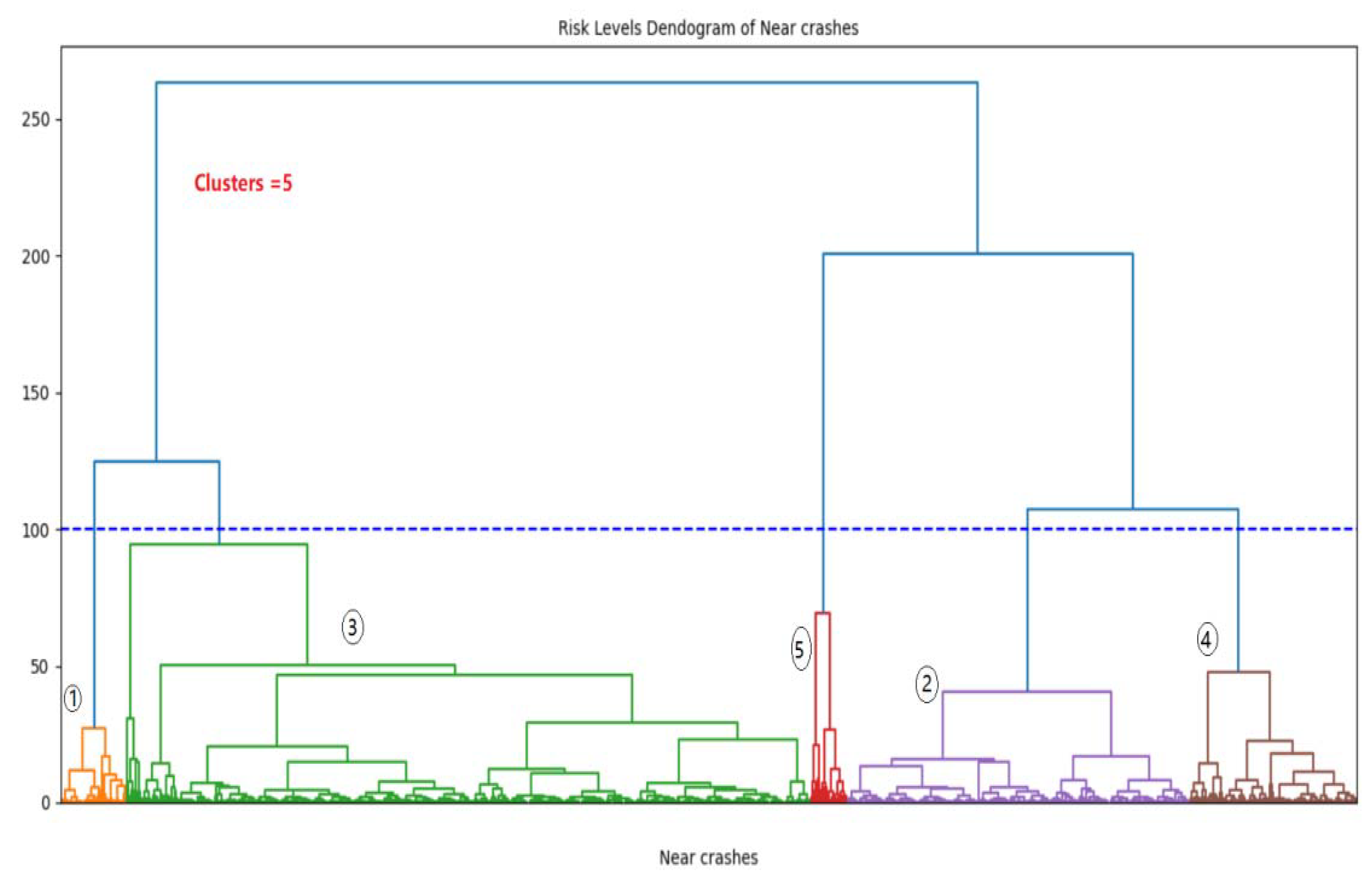
We used the testing dataset to provide accurate clustering results to choose the appropriate linkage methods for hierarchical clustering. We found that Ward’s linkage method [51] was suitable for identifying the near-crash levels based on the driving risk variables. The clustering results are shown in the hierarchical clustering dendrogram in Figure 6.

In Figure 6, near-crashes are categorized using driving parameters into five categories (risk levels): minimal, slight, moderate, serious, and severe. These categories are represented by 1, 2, 3, 4, and 5, respectively. Minimal and slight clusters have a lower risk proportion, by 31.5%. The moderate cluster has the highest rate of crash events at 52.8%, whereas serious and severe clusters are considered high-risk clusters at 12.9% and 2.8%, respectively. The severe cluster has a small number of near-crashes (46 events), which was expected.

To understand the distribution of the near-crash clusters (risk levels),

Table 4. Comparison of Hierarchical Clustering Results.

Number	Level	Near-Crash Events	Percentage (%)
1	Minimal	86	5%
2	Slight	411	26.5%
3	Moderate	882	52.8%
4	Serious	215	12.9
5	Severe	46	2.8%

summarizes the proportions of the five risk levels.

4.3.2. Feature Selection Results

In this study, lasso regression was developed and implemented using R statistical Software along with glmnet and caret packages.

Table 5. Estimation results for the lasso model.

Factor	Coefficients	Factor	Coefficients
Driving Behavior Features		Time Features
Beginning Speed	-	Time of Day
Average of Deceleration	−0.0018	1. 60:00–12:00	-
Average of Speed	0.0124	2. 12:00–18:00	−0.0561
Time Headway Average	-	3. 18:00–24:00	0.0171
Braking Pressure Average	-	Weekend
Min Deceleration	-	0. No	0.0165
Min Time Headway	-	1. Yes	0.0354
Max Braking Pressure	0.0298	Peak Hour
Vehicle Kinetic Energy	−0.0103	1. Yes	-
Road Features		2. No	-
Road Type		Near-Crash Features
1. Expressway a	-	Near-Crash Reason
2. Freeway	0.0408	1.Head-vehicle abruptly halted	−0.0192
3. Urban Expressway	-	2. Traffic Signals	-
4. Urban Road	−0.0092	3. Traffic Jam a	−0.0358
Road Congestion		4. Road Repairs	0.0154
0. Yes	−0.0158	5. Road changes	-
1. No	-	6. Pedestrians	-
Wet		7. Subject-Vehicle turned-off	−0.0483
1. Wet	-	8. Object-Vehicle turned-off	-
2. Dry	-	Near-crash Type
Light		Subject-Vehicle(Head) vs. Object-Vehicle (Head) a	-
1. Light	-	Subject-Vehicle (Head) vs. Object-Vehicle (Tail)	−0.0141
2. Dark	0.0174	Subject-Vehicle (Head) vs. Object-Vehicle (Side)	-
Weather		Subject-Vehicle (Side) vs. Object-Vehicle (Side)	-
1. Sunny	-	Subject-Vehicle (Side) vs. Object-Vehicle (Tail)	−0.0045
2. Rain	0.0244	6. Conflict with Pedestrian	-
3. Cloud	-	7. Parts of Road	-
Driver Features
Age		Education level
1. Less than 23	−0.0218	1. Less than graduate	-
2. 23–45 a	-	2. Graduate a	-
3. More than 45	−0.0373	3. Post-graduate and above	-
Gender		Driving Mileage	−0.0293
1. Male	-	Driving Experience (years)	−0.0164
2. Female	0.0172

^a Base reference of a categorical variable; - non-significant variable

shows that lasso regression fits the most significantly important variables with only non-zero values and ignores the variables by setting the coefficients exactly to zero. Using these significant variables as input vector X and the five near-crash events as labels Y, the dataset is ready for the training and testing procedure by the classification models introduced in Section 3.3.

Table 5 shows the covariates selected and their estimated coefficients, using all 1670 observations in the learning process. Covariates whose coefficients are large in terms of their absolute value have a great influence on the diagnosis of risk levels in near-crashes.

4.3.3. Model Comparison

(1) Classification Performance

We used the five risk levels of near-crashes obtained by hierarchical clustering as output labels to evaluate classification performance and the significant variables selected by lasso regression as the input vector. In other words, we aimed to train classification models that learn to map the collected variables of a near-crash to its risk level and then compared the performance measures for models built on the dataset with different levels of driving risk.

Firstly, the dataset was split into training data (80%) and testing data (20%). Secondly, the adopted classification models were trained by training data, and the classification performance was evaluated over the testing data. Finally, we used a confusion matrix to calculate the evaluation metrics, as shown in Equations (14)–(17). In what follows, the results of evaluation metrics, namely, accuracy, recall, precision, and F1-measure, are described. The accuracy performance results of each classification model are shown in

Table 6. Accuracy performance in classification models.

Model	Risk Levels of Near-Crashes
	Minimal	Slight	Moderate	Serious	Severe	Average
Support Vector Machine (SVM)	0.89	0.93	0.89	0.65	0.76	0.83
Random Forest (RF)	0.85	0.82	0.84	0.81	0.77	0.82
Multi-Layer Perception (MLP)	0.84	0.89	0.76	0.95	0.97	0.88
Ordinal Probit Model (OP)	0.80	0.72	0.90	0.82	0.80	0.81
Mutlinominal Logit Model (MNL)	0.71	0.77	0.76	0.84	0.80	0.78
Long-Short-Term Memory (LSTM)	0.93	0.94	0.85	0.93	0.96	0.96
Gated Recursive Unit (GRU)	0.96	0.87	0.75	0.94	0.98	0.91

.

In Table 6, numbers in bold denote the maximum value of a column, whereas the underlined numbers represent the minimum value.

Table 5 shows that MLP, LSTM, and GRU achieved the highest accuracy, and LSTM attained the highest average accuracy for minimal, slightly serious, and severe risk levels. The lowest accuracy was performed by the SVM at serious and severe risk levels, whereas the MNL had the lowest values in the minimal level and in average accuracy. For the prediction results of the moderate level, the OP model shows a high accuracy, and GRU achieved the lowest accuracy; this result might mean that the models that are relatively affected lost the capability of recognizing the moderate level, as it had the highest proportion.

The average accuracy ranged from 0.78 to 0.96. OP and MN achieved the worse accuracy. Among these models, the MNL had the smallest value for the testing dataset. The machine learning methods, i.e., the SVM, RF, and MLP, performed better than the statistical methods. For instance, the multilayer perception (MLP) obtained 0.88. Deep learning methods LSTM (0.96) and GRU (0.91) provided the most accurate performance.

By comparing the average accuracy of LSTM and GRU with previous studies, we found that the classification accuracy of our study achieved higher results than the prediction accuracy of similar studies, as shown in

Table 7. Accuracy performance comparison with previous studies.

Reference	Method	Accuracy
Wang et al. [3]	Classification Regression Tree (CART)	66.1%
Alkheder et al. [52]	K-means clustering based NN	74.6%
Assi et al. [51]	Fuzzy c-means clustering based SVM	74%
	Fuzzy c-means clustering based NN	71%
Mokhtarimousavi et al. [9]	Cuckoo Search based SVM	89.4%
Osman et al. [26]	AdaBoost	95%
Our Study	Long-Short-Term Memory (LSTM)	96%
	Gated Recursive Unit (GRU)	91%

.

The LSTM model in our study outperformed all state-of-the-art models. The LSTM achieved an average accuracy of 96%, which is followed by a 95% accuracy in Osman’s study [51] using AdaBoost. The GRU model also obtained high accuracy, at 91%. These findings indicate that deep learning and machine learning methods can effectively perform crash-related classification and prediction.

The above accuracy results may provide evidence that accuracy alone is not enough to evaluate classifier performance, so there is a need to study the results of other model metrics as well.

The performance of recall, precision, and F1-measure of the seven classifiers were calculated and are shown in

Table 8. Recall performance of classification models.

Model	Risk Levels of Near-Crashes
	Minimal	Slight	Moderate	Serious	Severe
Support Vector Machine (SVM)	0.76	0.82	0.75	0.82	0.85
Random Forest (RF)	0.84	0.87	0.78	0.82	0.87
Multi-Layer Perception (MLP)	0.92	0.85	0.76	0.92	0.89
Ordinal Probit Model (OP)	0.76	0.7	0.73	0.87	0.74
Mutlinominal Logit Model (MNL)	0.71	0.72	0.72	0.76	0.76
Long-Short-Term Memory (LSTM)	0.95	0.95	0.88	0.92	0.91
Gated Recursive Unit (GRU)	0.94	0.92	0.91	0.95	0.91

,

Table 9. Precision performance of classification models.

Model	Risk Levels of Near-Crashes
	Minimal	Slight	Moderate	Serious	Severe
Support Vector Machine (SVM)	0.78	0.87	0.84	0.73	0.66
Random Forest (RF)	0.81	0.90	0.85	0.75	0.66
Multi-Layer Perception (MLP)	0.91	0.90	0.85	0.80	0.75
Ordinal Probit Model (OP)	0.68	0.84	0.81	0.81	0.68
Mutlinominal Logit Model (MNL)	0.64	0.81	0.80	0.78	0.62
Long-Short-Term Memory (LSTM)	0.93	0.92	0.91	0.86	0.79
Gated Recursive Unit (GRU)	0.92	0.82	0.82	0.81	0.78

and

Table 10. F1-measure performance of classification models.

Model	Risk Levels of Near-Crashes
	Minimal	Slight	Moderate	Serious	Severe
Support Vector Machine (SVM)	0.77	0.85	0.82	0.78	0.74
Random Forest (RF)	0.82	0.88	0.83	0.78	0.75
Multi-Layer Perception (MLP)	0.91	0.87	0.83	0.85	0.81
Ordinal Probit Model (OP)	0.72	0.75	0.73	0.84	0.73
Mutlinominal Logit Model (MNL)	0.67	0.75	0.76	0.77	0.65
Long-Short-Term Memory (LSTM)	0.94	0.94	0.92	0.89	0.85
Gated Recursive Unit (GRU)	0.93	0.87	0.86	0.88	0.84

.

It is clear that the LSTM model, among the seven models compared, has the highest recall, precision, and F1-measure for each risk level. In contrast, the MNL usually achieved the lowest values.

In particular, as Table 8 shows, LSTM attained the highest recall value for all risk levels, ranging from 0.91 to 0.95, and MNL’s values were the worst, ranging from 0.62 to 0.81. In addition, it is clear in Table 7 that the severe level had the highest values, whereas the moderate risk level had the lowest ones. Thus, the LSTM model performed well for multi-class classification problems.

Table 11. Overview of the classification comparison measures.

Model	Average Accuracy	Average Recall	Average Precision	Average F1-Measure
Support Vector Machine (SVM)	83%	0.81	0.78	0.79
Random Forest (RF)	82%	0.84	0.79	0.81
Multi-layered Perception (MLP)	88%	0.88	0.84	0.86
Ordinal Probit Model (OP)	81%	0.77	0.76	0.77
Mutlinominal Logit Model (MNL)	78%	0.72	0.73	0.72
Long-Short-Term Memory (LSTM)	96%	0.93	0.88	0.91
Gated Recursive Unit (GRU)	91%	0.93	0.83	0.88

provides a summary of findings of the classification models, in regard to the average values of accuracy, recall, precision, and F1-measure. It is noted that larger values of the metrics indicate a better performance.

(2) Comparison of Running Time

We estimated the running time by the six models (i.e., SVM, RF, MLP, OP, MNL, LSTM, and GRU) in terms of the training loss, validation loss, and running time.

Table 12. Comparison of time efficiency.

Model	Training Loss	Validation Loss	Training Time (s)	Testing Time (s)
Support Vector Machine (SVM)	0.010	0.010	7.31	2.07
Random Forest (RF)	0.000	0.000	8.40	2.59
Multi-layered Perception (MLP)	0.007	0.006	10.27	3.21
Ordinal Probit Model (OP)	0.004	0.002	3.22	2.52
Mutlinominal Logit Model (MNL)	0.011	0.09	4.51	3.31
Long-Short-Term Memory (LSTM)	0.005	0.006	11.76	3.44
Gated Recursive Unit (GRU)	0.004	0.003	11.68	3.22

shows that all of the benchmarked models achieved better results; thus, these models can be used for the evaluation of real-time data from vehicles.

As shown in Table 12, the training time ranged between 3.22 and 11.76 s, whereas the testing time was between 2.07 and 3.44. Unlike the findings in the metrics of accuracy performance, the ML models, SVC, and RF required higher computational costs compared to statistical models. The DL models, such as the LSTM, provided the highest running time compared to the ML models. This can be interpreted as the structure of the neural network, which in turn increases the consumption time for the training and testing process. However, the running time results are acceptable and can be useful for real-time classification.

Regarding the relationship between the validation loss and training loss, there are slightly different results among the classification models. For instance, SVM, MNL, and MLP have higher loss values in the training and validation loss, whereas the RF model shows the best results. LSTM and GRU recorded better results as the network dropout has been modified to be 0.5 and 0.4, respectively.

In general, the results indicated that there is no overfitting or underfitting during the training and testing process.

5. Discussion

In this section, we discuss and compare this study to similar studies to show similarities and differences.

For the sake of grouping near-crashes into several high-risk groups, studies [3,4] have adopted k-means clustering analysis, which resulted in three driving risk levels, namely, low, medium, and high. In this study, near-crashes are grouped into five risk levels based on their driving behavior variables: minimal, slight, moderate, serious, and severe. Clustering results show that five levels better describes driving risk than three levels. This result conforms with [34].

Variable selection methods are used to consider significant variables for classification modeling and ignore unrelated variables. To do this, adaptive lasso regression was applied to the near-crash data. In [3], the authors adopted the classification and regression tree model and found several contributing factors, including a triggering variable, the object vehicle type, velocity of braking, and the crash type. In contrast, our study resulted in more contributing variables, such as average deceleration, average speed, kinetic energy, road type, the time of day, whether it was the weekend, the near-crash reason, the near-crash type, the driver’s age, the driving mileage, and driving experience. These variables can surely support classification modeling and provide more details for driving risk analysis of near-crashes. The findings of adaptive lasso regression are consistent with the results in [4].

As the results in Section 4.3 show, the machine and deep learning models achieved a better classification performance for near-crash risk than the statistical models. The statistical models that achieved weaker classification performance confirm the results in [40,51]. The low performance of the statistical models may be due to the linear nature of the adopted utility functions, and the distribution assumption of the error terms may not be necessary for near-crash data. The MNL could not consider the ordered nature of near-crash risk levels, while the OP model could determine the order of risk levels. The results show that the classification accuracy of the OP model was lower than that of the MNL model. Although the MNL model cannot consider the order of risk, the MNL model has an advantage over the OP model; the variables related to each driving risk level can be different, and each level can increase or decrease accordingly.

In the machine and deep learning models, the distribution features of the dataset and the correlation among the inputs and outputs variables did not need to be known in advance. The ML and DL models can learn the driving patterns from the training data, consider the order of near-crash risk levels, and enhance prediction accuracy.

In particular, the LSTM and GRU were the best models with the highest overall accuracy, at 96% and 91%, respectively.

The LSTM model would be the best option for classifying near-crashes from a practitioners’ perspective. It achieved the best overall performance in all five risk levels. The findings of the LSTM performance are consistent with the results in [46].

SVM and MLP were the next best performances, after the deep learning methods (LSTM and GRU). Table 8, Table 9, Table 10 and Table 11 show that the SVM model performs the best in predicting near-crash risk levels, followed by the MLP. The ML models have better classification accuracy for a small proportion of data compared to the OP and MNL models. This finding confirms the results of the crash risk severity of the studies [15,51].

To the best of our knowledge, despite the considerable research efforts on driver behavior analysis using ML algorithms, there are no similar comparative studies of both ML and DL algorithms in predicting and classifying the driving risk levels of near-crashes.

There are several limitations in this study. Firstly, while the dataset size in this study (n = 1690 near-crash events) is acceptable and near to the magnitude of data in several similar studies [27,34], it is smaller in magnitude than the study reported in [26,29]. Secondly, there is a need to append related datasets (such as real crash datasets) to provide more comprehensive results. Thus, classification models could potentially achieve higher accuracy and better results. Thirdly, there is a need to add significant kinematic variables such as YAO and longitude acceleration, which could provide a deeper understanding of driving behavior in relation to near-crashes.

6. Conclusions

Recently, crash risk analysis has attracted considerable attention from researchers, governments, and decision-makers aiming to enhance safety and reduce fatalities, injury, and damage. However, crash risk classification and prediction is not a trivial issue and requires higher quality and larger datasets to efficiently train models that can reliably predict crashes and related events.

Due to the small size of the crash dataset, many researchers have considered using near-crash events as surrogate measures for real crashes. In this study, a near-crash dataset was collected by conducting a naturalistic driving experiment with related data sources such as driver input, temporal data, and geometry data. The near-crash events were extracted by exploring driving behavior variables. To facilitate the classification procedure, five risk levels were obtained by applying hierarchical clustering on near-crashes. Adaptive lasso regression was utilized to select significant variables indicating the performance of classification models of near-crashes. To develop the classification models, 80% of the data was used for the training phase, 20% for the testing phase. The study compared the classification performance for near-crash risk levels among various statistical, machine, and deep learning models. Performance metrics included accuracy, precision, recall, and F1-measure.

The results showed that machine and deep learning models (MLP, LSTM, and GRU) achieved considerably better classification accuracy performance in predicting near-crashes risk levels.

Overall, the only model that obtained a reliable performance at predicting near-crashes and normal driving was the LSTM. The LSTM model achieved a remarkably high prediction accuracy of 96% at all risk levels. Moreover, high values were achieved by the LSTM (recall = 0.93, precision = 0.88, and F1-measure = 0.91).

In addition, the results showed that the LSTM model is a promising tool for classifying the risk levels of near-crashes. This could be used in real-time driving to identify and determine the risk level of near-crashes and thus enhance overall safety. The findings of this study can provide insights supporting crash avoidance systems and developing more targeted programs for driver training. In addition, driver monitoring systems may help to reduce the secondary task involvement, leading to a decrease in the incidence of critical events, as well as forward collision.

In future studies, we intend to obtain lateral acceleration, longitudinal acceleration, and YAO rates. We recommend incorporating more characteristics in the violation data for the identification of the groups at a higher risk of future violations and future crashes. Future studies could also match more violation types as crash types to identify the groups at a higher risk of each of the crash types. In addition, there is a plan to consider other significant variables that can contribute to crash risk, i.e., distractions such as mobile phones, driver fatigue, and unhealthy lifestyles.