Abstract
Climate change is affecting more and more local communities, which are now facing different hazards; in answer to this threat, specific actions at the local level should be taken. The Covenant of Mayors (CoM) is an initiative that tries to involve municipalities and communities in developing SECAPs, i.e., plans for sustainable energy and climate with the aim to develop adaptation and mitigation measures. In order to identify and evaluate hazards, the CoM developed a template relative to the current risk level and expected changes in the future. This paper develops a methodology to fill the template using a data driven approach instead of a heuristic one. The methodology was applied to the city of Trieste in northeast Italy and uses local weather station data and projections obtained from GCM-RCM models. Data were manipulated using different approaches for current risk levels and the Mann–Kendall test is proposed as a method to identify the future evolution of hazard intensity and frequency. The results showed that the developed approach could help municipalities in developing their SECAPs and in identifying the present and future evolution of hazards.
Keywords:
climate change; hazards; mitigation; regional climate models; municipality; SECAP; SEAP; Covenant of Mayors 1. Introduction
Climate change is becoming more and more of a concerning problem for a variety of sectors, such as buildings, agriculture and healthcare. The growing trend in temperature has been widely assessed throughout many studies in the last few years and a valuable summary of this research can be found in the 2021 Sixth Assessment Report of the Intergovernmental Panel on Climate Change [1]. That document reports that the global surface temperature was 1.09 °C higher in the 2011–2020 period than in the 1850–1900 one, showing an additional estimated increase in global surface temperature since the AR5 report. This strong increase is said to be due to the anthropogenic greenhouse gas emissions, which trap solar radiation in the atmosphere, thus causing excessive warming. In Europe, temperatures will rise at an increasing rate [2], leading to a rising frequency and intensity of extreme heat events, with a decrease in cold spells. Precipitation is expected to decrease in Mediterranean area; however, extreme precipitation and flooding events are predicted. Other effects have been identified, such as rising sea levels and a decline in glaciers [3].
Europe has set a new growth strategy with the European Green Deal [4], with the ambitious project set to achieve climate neutrality by 2050 with an intermediate step of emissions reduction of at least 55% by 2030. Different actors can contribute to achieve these objectives, and, furthermore, municipalities can directly drive climate change mitigation actions [5] since they can implement mitigation and adaptation policies closely related to urban sustainable development.
The Covenant of Mayors (CoM) presented itself as the mainstream European movement for local climate and energy actions involving local authorities by signing a Sustainable Energy Actions Plan (SEAP), committing to increase energy efficiency and the use of renewable energy sources. Although there were some difficulties in implementing SEAPs [5,6,7], the results confirm the great potential of the CoM initiative to contribute to mid-century climate change mitigation targets, as reported by Kona [8], which highlights that the CoM signatories would be in line with the 1.5 °C global target scenario.
In 2015, the integration of climate adaptation and mitigation aspects within the SEAPs led to the development of Sustainable Energy and Climate Actions Plans (SECAPs). Looking at the Italian scenario, Pietrapertosa [9] found that 61 out of 76 cities developed municipal civil protection plans as instruments to deal with local emergencies associated with extreme weather events. He focused on the fact that, in the absence of a national law that imposes the development of climate plans, transnational networks, such as CoM, are an effective tool for a voluntary commitment to reach EU climate and energy objectives. With this target, Jekabsone [10] proposes an integrated approach for involving stakeholders from the beginning of the development of SECAPs, applying it to the experiences of six communities.
One of the main aspects of the development of SEAPs into SECAPs is the analysis of the effect of climate change on the plans of the communities. As such, when developing a SECAP, a Climate Change Risks and Vulnerabilities Assessment (RVA) should be performed with an effort to identify and evaluate relative hazards. However, no unique approach could be identified in the literature. Guides are available to help municipalities develop SECAPs from SEAPs, with references on how to identify hazards [11] based on available data. A frequently adopted approach is to use qualitative risk analysis based on expert judgment, but if some data is available, it is recommended to use quantitative methods instead. Nowadays, climate projections using climate projections from GCM-RCM for several weather-related quantities can be obtained [12], and they can be utilized to explore future trends in climate variables and related hazards. However, the future behavior of hazards appears to be mainly based on personal judgment and also visual analysis of maps, if based on numerical projections. In some cases, the trend is quite simple to identify. The MasterAdapt project [13] carried out an analysis of the Sardinia Region for scenarios RCP 4.5 and RCP 8.5; in this case, the trend for temperature related hazards could be clearly identified, but precipitation revealed no clear trend. Interestingly, in the same document, the analysis of past events was supported by a numerical approach by applying the Mann–Kendall test [14] in order to retrieve an unequivocal behavior. A similar visual approach was carried out in [15] for the SECAP of San Donà di Piave, where, for future temperatures and tropical night anomalies, an increase in frequency and intensity were identified by inspecting a table reporting the RCP 4.5 and 8.5 scenarios. Other papers simply avoid mentioning the method used for defining the future hazard trend; in [16], only the presence of a hazard report is included, but it signaled a scarcity of data related to downscaled data at regional and local scales. However, the future trend is generally identified by inspecting projections values for related areas and generally expressing the trend as an increase, strong increase or no trend. In [17], the authors determined the likelihood of extreme events by calculating the probability of exceeding a value using the Extreme Value Theory and plotted the difference between exceedance probability, computed using future scenarios, and historical data for far and near future periods; again, the future trend of hazards was taken visually by inspecting graphical maps. However, in [18], the authors suggest reducing the uncertainty in climatic information provided to end users through the use of change detection tests.
In this paper, a practical methodology to assist the developers of SECAPs in identifying the future development of hazards, as requested by the completion of the CoM template, is introduced. The method elaborates data that can be recovered from available databases, using the Mann–Kendall test as a change detection approach to identify a possible future trend for each hazard as an alternative to the simple visual analysis of maps or tables. This work was conducted as part of the Italy–Slovenia SECAP project, “Supporting energy and climate adaptation policies” [19], which aims to develop a methodology for allowing communities to develop SECAPs from SEAPs within a transnational, cross-border framework. The methods presented here were applied to the city of Trieste, for which a SECAP was conceived during the development of the project.
2. The CoM Template
When drafting a SECAP, although there is not a fixed framework, a suggested approach is to follow the Covenant of Mayors reporting template [20]. The document includes different sections that a signatory must fill out in order to complete the plan. The template is a workbook with tabs related to different parts of a SECAP: Strategy, GHG Emissions, Target Setting, Risk and Vulnerability Assessment, Reporting on Progress: Mitigation and Adaptation Actions Inventory, Energy Poverty Plan. In this work, we focus on the Risk and Vulnerability Assessment Table. Although the data is provided for the City of Trieste, northeast Italy, the proposed method could be applied to different cities or municipalities as well, with the only limitation being the availability of historical weather data and climate data projections.
The form, presented in Figure 1, is divided into two main sections dealing with “Current risk of hazard occurring” and “Future hazards”. While the former can be filled using information available at the municipal or regional level, the “Future hazards” sector is quite difficult to fill out if it is not using heuristic methods based on the local experience [21]. The current hazard risk is defined by “Probability of hazard” and “Impact of hazard”, which can be calculated based on previously available climate data. However, the part related to “Future hazards” is more problematic, as information about the fields “Expected change in hazard intensity”, “Expected change in hazard frequency” and “Timeframe(s)” are mandatory. These require knowledge of future climate behavior and a coordinated method for extracting and processing climate data. Regarding the future climate, Global Climate Models (GCM) coupled with Regional Climate Models (RCM) can be viewed as a precious information source that can provide data allowing the evaluation of the future risk in a particular site [21,22].
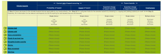
Figure 1.
CoM template, Risks and Vulnerabilities Tab.
2.1. CoM Template Filling
A standardized process to define the distribution for past and future events of each climate hazard is helpful in determining the Risk and Vulnerability Assessment (RVA) and, therefore, to fill the template. The process first determines the actual risk of danger, then, following the Reporting Guidelines of the Covenant of Mayors [23], defines two parameters that represent the actual level of risk:
- Probability of hazard;
- Impact of hazard.
Both parameters have four different levels of importance that are associated with: High, Moderate, Low and Not Known. To determine these levels for the probability of hazard, the instructions proposed by the Guidelines have been utilized, with the definition of each level represented in Table 1.

Table 1.
Probability of hazard definition.
To evaluate the future risk of danger due to these events, three parameters are used in the Risk and Vulnerability Assessment:
- Expected change in hazard frequency;
- Expected change in hazard intensity;
- Timeframe(s).
As to the concerns of the first two parameters, the guidelines of the Covenant of Mayors provide a choice between three options: Increase, Decrease and Not Known. However, no instructions are reported on how to choose between the proposed options. Regarding the timeframes in which the changes are expected, the guidelines define three periods:
- Short-Term: within 20–30 years from now;
- Mid-Term: after 2050;
- Long-Term: within the 2100s.
2.2. Weather Data for Friuli Venezia Giulia Region
Along with historical data provided by Regional Agency for the Protection of the Environment (Agenzia Regionale per la Protezione dell’Ambiente del Friuli Venezia Giulia—ARPA FVG) in local weather stations, future projections have been used to fill out the Risk and Vulnerability Assessment (RVA) section of the template in a systematic way.
For the Italian region Friuli Venezia Giulia (FVG), ARPA FVG published the “Cognitive study of climate changes and of their impacts in Friuli Venezia Giulia” [24]. This document deals with past and future climate changes in the FVG region; furthermore, the data of several GCM-RCM models for the area were produced and made available to the public. Since many coupled Global–Regional models are available on the CORDEX project platform [12], the ARPA FVG document chose the ones considered the most representative for the Friuli Venezia Giulia Region area. The models resulted from the dynamic downscaling of regional models on the EUR-11 Cordex domain [24]. The selected models are presented in Table 2 along with the elaboration institution.
Table 2.
GCM-RCM models identified by ARPA for Friuli Venezia Giulia Region.
The downloaded files provide daily data for various climatic variables for a historical period from 1971 to 2005 and future projections from 2006 to 2100 using Representative Concentration Pathways (RCP) 8.5, 4.5 and 2.6. The files reported average daily data for the considered variables, but for temperature data, the files reported the daily maximum, minimum and average temperature.
2.3. Data Required for Template Filling
In this paper, the reported method was tested for the municipality of Trieste and for the following climate hazards:
- Precipitation-related hazards:
- Heavy precipitation;
- Drought and water scarcity;
- Wildfires.
- Temperature-related risks:
- Heatwaves;
- Cold spells;
- Frost days.
- Geological hazards:
- River flood;
- Coastal flood and storm surge;
- Landslide and rockfall.
The climatic indices used to quantify each climate hazard were calculated from climate data retrieved from different sources, as reported in Table 3. Different approaches can be identified to fill the CoM template depending on the kind of hazard considered.
Table 3.
List of hazards and their related frequency and intensity indices along with the data sources used in the framework for CoM template-filling. GCMs = Global Circulation Models, GEFF = Global ECMWF Fire Forecasting model.
In the following section, each hazard will be considered separately, and the filling of the relative part of the CoM template will be identified.
3. Precipitation Related Hazards
For “Heavy precipitation” and “Drought and water scarcity” hazards, climate data were retrieved from three GCM-RCMs, namely, models M1, M3 and M4 of Table 2. We selected only three GCM-RCMs, since it is the minimum number suggested for future projection analyses by the data provider (International Centre of Theoretical Physics, ICTP, Trieste, Italy).
3.1. Heavy Precipitation
The following indices were calculated to quantify the frequency and intensity of “Heavy precipitation”, as they have been widely included in previous studies on extreme precipitation events [25,26,27]:
- R20mm, or very heavy precipitation days: number of days where rainfall (RR) ≥ 20 mm. Let RRij be the daily precipitation amount on day i in period j; count the number of days where RRij ≥ 20 mm;
- RX5day, maximum five-day precipitation: highest precipitation amount in five-day period. Let RRkj be the precipitation amount for the five-day interval k in period j, where k is defined by the last day. The maximum five-day values for period j are RX5day, j = max (RRkj).
R20mm was calculated by counting the number of days with precipitation > 20 mm using a custom made function (code available upon request), while the RX5day index was calculated using “climdex.rx5day” function in the “climdex.pcic” package [28].
3.2. Drought and Water Scarcity
The “Drought and water scarcity” hazard was quantified on the basis of:
- Self-calibrating Palmer Drought Severity Index (scPDSI) [29], which has been previously used to calculate the frequency of drought extremes [30,31,32]. It automatically calibrates the behavior of PDSI at any location by replacing empirical constants in the index computation with dynamically calculated values;
- Consecutive Dry Days (CDD), which have been previously used to calculate the intensity of drought extremes [33]. It is defined as the maximum length of a dry spell, i.e., the maximum number of consecutive days with RR < 1 mm.
scPDSI was calculated from monthly precipitation (in mm) and a potential evapotranspiration (PET, mm) series. Monthly precipitation was calculated from daily precipitation data form GCMs. Monthly PET was calculated according to a modified version of the Hargreaves equation [34], provided by Droogers and Allen [35], which computes the monthly reference evapotranspiration of a grass crop, corrected using the amount of rain for each month as a proxy for insolation. In detail, PET was calculated through the “Hargreaves” function in the “SPEI” R package [36] from the monthly mean minimum and maximum temperature and the monthly precipitation computed from GCMs. Finally, scPDSI was calculated using the “PDSI” function in the “scPDSI” R package [37]). CDD was computed from monthly precipitation (in mm), using the function “exceedance” in the “RmarineHeatWaves” R package [38].
3.3. Wildfires
To quantify the hazard of “Wildfire”, a slightly different approach was used. Specifically, we utilized the Fire Weather Index (FWI) [39], which is a dimensionless, meteorologically-based index used worldwide to estimate fire danger in a generalized fuel type (mature pine stands). Currently, FWI is applied in several European national and regional public bodies (e.g., France or ARPA Piemonte, respectively), and it became the official index for the operational, medium-range fire danger forecasts issued by the European Forest Fire Information System (EFFIS) [40]. FWI was implemented using the Global ECMWF Fire Forecasting model (GEFF). The output is a gridded version of future fire danger projections (resolution 0.11° × 0.11°) under the umbrella of the Copernicus program [41]. The dataset was developed using three-hourly climatic output from state-of–the-art GCM/RCM pairs (CNRM-CM5, EC-EARTH, IPSL-CM5A-MR, HadGEM2-ES, MPI-ESM-LR, NorESM1-M) developed within the EURO-CORDEX initiative [12]. Data consists of daily FWI values computed on the historical aspect (1970–2004) along with future projections (2005–2097), which were based on the Representative Concentration Pathways (RCPs) 2.6, 4.5, and 8.5. The following indices were computed:
- Seasonal FWI (sFWI), which represents the average FWI values for the June–September period (considered “Fire season” in the Northern Hemisphere);
- N15, N30 and N45, describing the number of days with moderate, high and very high fire danger conditions according to EFFIS scale [42]. Data for the municipality of Trieste were obtained from the EFFIS website.
Simple moving averages (SMAs) were calculated in the historical scenario in order to assess average values over multiple periods (here, time windows k = 4, k = 8, k = 13) to determine the current probability of occurrence of the hazard. SMA is a smoothing approach that averages values from a window of consecutive time periods, thereby generating a series of averages based on different smoothers in order to reduce the noise and uncover patterns in the data.
4. Temperature Related Hazards
Temperature values recovered from weather stations and the models in Table 2 were used to develop indices for “Extreme Heat” and “Extreme Cold” hazards. The data obtained from models referring to the historical period may differ from data collected in weather stations for the same time slice. In order to improve the predictions, the future data of models were modified before use in order to evaluate climatic trends, since they may influence the expected climatic impact, creating a bias error [43,44]. The correction was carried out using the available measurements of weather by using a quantile mapping approach [45,46], assuming that biases in historic observations would be repeated during the projections. The correction was carried out for mean daily temperature, minimum daily temperature and maximum daily temperature.
To avoid inconsistencies, the approach of Thrasher et al. [45] was followed in this work, applying quantile delta mapping [46] to maximum temperature and to the difference between maximum and minimum temperature, preserving the relative and absolute changes in modeled quantiles. The modified data was used to develop the metrics related to temperature hazards considered in this paper: heatwave (HW), cold spell (CS) and frost days (FD).
4.1. Heatwave
In the literature. there is not a unique definition of heatwave; for the present work, the definitions available in Casati et al. [47] and Robinson [48] were used, and the parameters were computed using the Python package xclim [49]. The heatwave is described here as an event where minimum and maximum daily temperature are higher than 22 °C and 30 °C, respectively, for three consecutive days. To evaluate climate change, the following parameters related to HW were considered:
- Heatwave frequency, HWfreq, defined as the number of events in a year;
- Heatwave maximum length, HWlen,max, defined as the maximum number of days pertaining to a HW consecutively;
- Heatwave total length, HWlen,tot, defined as the sum of days that fall into a heatwave in a predefined period.
4.2. Cold Spell and Frost Days
Other parameters of interest when dealing with hazards related to temperature are those relating to extreme cold: cold spells (CS) are events characterized by a mean daily temperature lower than a given threshold (in this work, set to −5 °C) for three consecutive days. Frost days (FD) are instead defined as ones where the minimum daily temperature falls below 0 °C. The severity of climate, in this case, is evaluated by computing:
- Cold spell frequency, CSfreq, that is, the number of cold spells in a period;
- The maximum number of consecutive frost days, FDcons,max;
- The total number of frost days, FDtot.
5. Geological Hazards
Although global warming is undeniable [50,51], the impacts of global warming and related climate changes on geohydrological hazards (e.g., floods and landslides) remain difficult to detect and predict [52].
For example, Gariano and Guzzetti [52] found that three climate variables (air temperature, total rainfall, rainfall intensity), known to affect slope stability and landslides [53], as well as the geographical and temporal ranges of some landslide types, operate on different and only partially overlapping scales. This means that for different landslides, climate variables, geographical characteristics (extension of landslide, land use, etc.), the GCM/RCM scenarios considered and the time of reactivation, e.g., of a landslide cannot always intersect to forecast their future evolution.
The combined impacts of rising sea levels and possible increases in the frequency and intensity of storms make coastal zones particularly vulnerable to climate change [54]. Climate change is the primary cause of anticipated increases in coastal flood losses, with the role of coastward migration, urbanization and growing asset values progressively diminishing over time. A wide range of methodologies have been gradually developed in this direction, with approaches based on synthetic indices and indicators, or on dynamic representations of current processes at various levels of conceptualization, sometimes using GIS tools [55]. It has been demonstrated that visualizations of the land at risk of flooding due to rapid sea level rising are achievable and necessary for coastal vulnerability assessments using a digital terrain model and geographic information system (GIS) [56].
The LISFLOOD analysis is restricted to the larger rivers in Europe, which may not be representative of a whole country or region [57].
In this work, we provide a methodology for some geological hazards of the CoM template (river flood, coastal flood, storm surge, landslide and rockfall) based on the intrinsic geological characteristics and vulnerabilities of the territory through spatial analysis in order to quantify the cause-and-effect linkages specified by the CoM template. A holistic and multidisciplinary approach is required to understand and quantify how climate variables and their fluctuations affect geohydrological risks. However, each method was conceived and simplified to allow public administrations to more easily scale the current hazards using the attributes “Low, Moderate, High”, thereby avoiding the statistical methodology recommended in the Covenant of Mayors’ Reporting Guidelines. In fact, statistics on the frequency of such occurrences are not always available, particularly in the absence of up-to-date catalogues or databases. As a result, a strategy focused on the geography and the diversity of accessible data was deemed more appropriate to fill the template.
5.1. River Flood
In the CoM template, “river flood” is defined according to the WMO (World Meteorological Organization) as “a flood that occurs over a wide range of a river and catchment system, on flood plains or wash lands as a result of flow exceeding the capacity of the stream channels and spilling over the natural or artificial embankments”. This sentence is the focus of the PAIs (Piani di Assetto Idrogeologico, the Italian Hydrogeological Setting Plans), which are regulated and managed by the Basin Authorities, i.e., the Italian territorial authorities established following the implementation of Directive 2000/60/EC. A PAI contains an assessment of a territory’s hydraulic and hydrogeological hazards, as well as the areas that will be subject to protection measures, based on:
- 100-year Return Period (RP) events;
- Historical flood events;
- Specific flood patterns;
- Embankment condition and upkeep.
The hazard level classification is divided into four increasing levels (H1 to H4), while H0 indicates no exposure at all. This information can be pooled in GIS in order to assign a single hazard value for the entire municipality in terms of “Low–Moderate–High,” as the CoM template requires. Each territorial unit with a specified hazard (from an H0 area to an H4 area) according to the PAI is compared to the municipal total surface (Atot), and then weighted by a coefficient corresponding to the severity of the hazard (in a ranking order from 1 to 5), following a linear progression, to obtain a single reference value. As a result, for a specific municipality, the hazard indicator for “river flood” (HRF) is:
The result of this expression is a value between 1 and 5. According to experience and expert knowledge of the phenomenon, the values obtained are classified into three intervals corresponding to the “Low–Moderate–High” attributes (Table 4).
Table 4.
Levels of river flood hazard based on classification of HRF calculated using Equation (1).
When estimating the impact of a hazard, it is useful to analyze the vulnerability of an affected region to a prospective flood. In this regard, the European Union enacted Directive 2007/60/EC on the assessment and management of flood risks. This Directive mandates the creation of flood risk maps that show the potential negative implications of various flooding scenarios on the territory. According to the Italian regulations, maps are constructed using four risk classes, based on:
- PAI’s hazard categorization;
- Different RP of intense events;
- Land use of the flood-prone area.
In this work, we simplified the approach for determining the ranking of the impact using risk maps with a 100-year RP because the PAI are based on the same RP, and the predictive models used for the SECAP run up to 2100. Accordingly, the risk levels were converted in the attributes required by the CoM (Table 5). The same approach can be used to rank the level of hazard and its impact for the lower RP (i.e., 20-year or 50-year RP) if required.
Table 5.
Impact of river flood hazard, classified using the mapped risk levels available at the national level according to Directive 2007/60/EC.
The CoM requires a single attribute of the hazard impact for the municipal territory, even if the risk levels are more than one. Using the precautionary principle, the municipality was assigned the maximum impact ranking found within it in order to avoid underestimating those municipalities that, despite their small size, have a very high risk.
As far as the expected change in hazard frequency and intensity is concerned, we can apply the simple concept of cause-and-effect. According to [58], global warming will progressively increase flood frequency and severity in most of Europe, since heavy precipitation events are likely to increase in the worst climate change scenario (RCP 8.5). Since the product of the probability of events by the vulnerability of the elements at risk is a measure of hydrological risk, it is easy to see how the combination of a higher frequency of events and a greater vulnerability for the territory can cause disasters, which most often occur in areas where a high hydrogeological risk is known [59]. Therefore, only in the case of an ascertained increase in the indices of heavy precipitation (i.e., RX5day) in a given timeframe using a climate model does an expected change in flood frequency and intensity increase; otherwise, it is labeled as decreasing, no change, or not known, if appropriate.
5.2. Coastal Flood and Storm Surge
The WMO’s definition of a coastal flood as provided in the CoM template as “higher-than-normal water levels along the coast caused by tidal changes or storms that result in flooding, which can last from days to weeks”. Storm surge refers to “the temporary increase in the height of the sea due to extreme meteorological conditions (low atmospheric pressure and/or storm winds)”. Considering that coastal flooding is driven by the same forces as storm surges, accomplished via the meteorological component of tides, in the following sections, these topics will be discussed as a single argument. Hazard assessment for coastal flooding cannot be separated from the topography of the inundated land.
Accordingly, we adopted the same methodology of [60] by using the DTM (Digital Terrain Model, based on 2018 Lidar surveys conducted by the Italian Civil Protection Department of the coastal areas of interest, simulating a submergence due to a coastal flood that induces a sea level rise of +180 cm, associated with a scenario which has a 30-year RP [61]. This scenario accounts for the combined effect of a meteorological high tide, storm surge, and wave setup. The topographically exposed areas are extrapolated by considering only the direct connection to the sea. For the City of Trieste, this was extrapolated using the projected marine ingression to a minimum territorial region of flooding, characterized by critical flooding that occurs along at least a 1-km-long urbanized shoreline, extending for at least 20 m into the hinterland (that is, an area of 20,000 m2). A high impact zone was also established, with a 2.5-km-long shoreline and a 20-m penetration into the hinterland (that is, an area of 50,000 m2). Both areas might be unitary or a sum of smaller zones, and their sizes can be indicative of emergency management issues. Therefore, we propose to fill out the CoM template as follows:
- If the flooded predictive area is less than 20,000 m2 (area or sum of surfaces), the coastal flood hazard (HCF) is low;
- If the flooded predictive area is greater than 50,000 m2 (area or sum of surfaces), HCF is high;
- If the predicted flooding area is between 20,000 and 50,000 m2 and the flood penetrates for at least 20 m, HCF is moderate (Table 6).
Table 6. Levels of coastal flood hazard based on the total extent of the inundation area.
The resulting flood inundation maps are combined with exposure and vulnerability information in order to estimate direct flood damage [60]. To quantify the impact of the hazard, we used a GIS to overlay the previously established hazard layer with the MOLAND land use [62]. To simplify the process, we devised a geographical reclassification by merging some classes based on economic, social and cultural weights and defining the class of elements under risk, as indicated in Table 7.
Table 7.
Classification of element at risk based on the characteristics of the urban areas.
The impact of the hazard can be easily defined according to a matrix, which combines the level of hazard and the element at risk, as reported in Table 8.
Table 8.
Impact of the hazard, classified according to a matrix between the level of risk (Low–Moderate–High) on the left column, and the elements at risk (the four classes of Table 7). The impact is classified as Low–Moderate–High, as requested by the CoM template.
The combined effects of future sea level rises and subsidence along the coastal area of the northern Adriatic are well known [63,64,65]. As a consequence, the expected change to coastal flood frequency and intensity is not difficult to assess, even within specific timeframes.
5.3. Landslide and Rockfall
The CoM template, as with the previous hazards, uses the WMO’s definition of landslides, which is fairly generic and includes many forms of landslide according to Cruden and Varnes classification [66]. The CoM template also depicts rockfall, which is “the sudden and very rapid downslope movement of unsorted mass of rock and soil due to heavy rain or rapid snow/ice melt”. However, because the template does not include any other sorts of landslides other than rockfalls, it was decided that the latter should be included in landslides. The FVG Regional Cadaster of Landslides (which includes rockfalls as well) was chosen as a tool for analyzing national-scale activities (for example, PAIs). However, because the municipalities lacked a historical series of landslide activation and reactivation, an analysis of the available data was conducted (e.g., municipalities affected by landslides, the number of landslides in the municipality and the municipal area). When the frequency of landslides is compared in terms of number of events per municipality and number of events normalized to the extent of the municipality, as shown in Figure A1, it appears to be a significant representation of the phenomenon, because the first quantifies the events while the second defines the extent of the impact. The level of landslide hazard has been scaled on the basis of the correlation between the two indices, as reported in Table 9 and presented in Figure A2.
Table 9.
Levels of landslide hazard based on landslide frequency (number of landslides, N, per km2) and absolute number of landslides, N, recorded in any FVG municipality.
To define the hazard impact, we used the same procedure we applied to coastal flooding, overlapping the hazard layer in GIS with the reclassified land use (Table 7).
As for the other hazards, the CoM requires a single attribute of the impact on the municipal territory. We then assigned the municipality the maximum impact ranking related to the presence of a landslide in the most vulnerable area (highest score of the elements at risk), according to the precautionary principle.
Establishing a link between climate change and its possible consequences on incidences or lack incidences of landslides in a specific location is still a topic of debate. Although numerical models can simulate climatic variables, such as temperature and precipitation, and estimate the corresponding level of confidence, the way and extent to which projected climate changes may modify the response of single slopes or entire catchments, the frequency and extent of landslides and the associated variations in landslide hazard, remain unclear [67].
It is out of the scope of the present work to determine a specific relationship between climate variables and landslides, as well as the possible interferences with direct anthropogenic forces, since changes resulting from human activity are seen as a factor of equal, if not greater, importance than climate change in affecting the temporal and spatial occurrence of landslides [53].
Lacking a specific and more exhaustive analysis of the local phenomena [68,69,70], we decided to apply a cause-and-effect relationship for defining the expected change in landslide hazard, adopting the same principle as the river flood. If we consider a hydroclimatic landslide triggering model [53], we can assume that increases in rainfall intensity will lead to an increase in landslide activity [71]. Therefore, only in the case of an ascertained increase in the indices of heavy precipitation (i.e., RX5day) in a given timeframe using a climate model does the expected change in landslide frequency and intensity increase; otherwise, it is labeled as decreasing, no change or not known, if appropriate.
6. The CoM Template Completion for Trieste
In the previous section, the various hazards concerning the CoM template and the parameters used to quantify them were presented. In this section, the parameters will be computed for the SECAP of Trieste, and the template will be filled accordingly. Due to the number of hazards and parameters involved, tables and figures reporting the complete results have been presented in Appendix A for rain and temperature-related hazards and in Appendix B for geological ones.
Regarding rainfall and temperature-related hazards, to compute their probability, first, we computed the fraction of the total amount of days included in an event against the total number of days included in a reference period. The obtained value was used to define the probability using Table 1. Regarding the impact of actual extreme events, the choice of importance level should be delegated to municipalities, following what is reported in the guidelines.
In order to evaluate the future evolution of hazards, the modified Mann–Kendall trend test (MMKT) [14] was used. This test was first conducted on the frequency of extreme events, defined before as the total number of days included in an event compared to the total days of the reference period. The evolution of the frequency was then studied in relation to the five climatic models of Table 2 for each RCP scenario in the 2020–2045, 2046–2070 and 2071–2100 periods, representative of the Short, Mid and Long-Term, respectively. In addition to identifying the trend, the Theil-Sen (T.S.) indicator, representative of the change in magnitude of the analyzed event, was also computed. Only the test results with a statistical significance value, p, less than 0.05 were considered significant. Due to the size of the tables, the results of the MMKT are reported in Appendix A.
Geological hazards have been treated using a different approach; in this case, additional tables and figures are reported in Appendix B.
For each hazard, the current analysis for Trieste is presented in the following sections.
6.1. Heavy Precipitation
In the municipality of Trieste, the current probability of occurrence for heavy precipitation, expressed in terms of R20mm, is moderate, since it was considered close or equal to 0.05 in all the three GCMs, as shown in Table 10.
Table 10.
Heavy precipitation (R20mm) current probability of occurrence considering the historical scenario calculated from daily precipitation data provided by the three GCMs (M1, M3, M4) for the city of Trieste.
Regarding future projections, the frequency of heavy precipitation will probably not change, since no trend in R20mm was detected in any GCM, as reported in Figure 2 and in Table A1. Conversely, the intensity of heavy precipitation (RX5day) will increase under the RCP8.5 scenario, since all the GCMs converged in detecting a significant positive trend, as reported in Figure 2. Moreover, in all the three GCMs, the increasing trend will likely occur in the Long-Term timeframe (2071–2100), as detected via the MMKT, reported in Table A2.
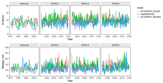
Figure 2.
Temporal variation of the number of days with precipitation > 20 mm (R20mm) and maximum five-day precipitation (RX5day) indices considering historical and future scenarios (RCP2.6, RCP4.5, RCP8.5) calculated from daily precipitation data provided by the three GCMs (M1, M3, M4).
6.2. Drought and Water Scarcity
In the municipality of Trieste, the current probability of occurrence of moderate and severe drought, expressed in terms of scPDSI, is High, since all three GCMs showed a current probability greater than 0.05 (Table 11). Regarding extreme drought, the first two models detected a high probability of occurrence, greater than 0.05, while the third one (M4) showed a lower value—less than 0.005—as reported in Table 11.
Table 11.
Droughts and water scarcity current probability of occurrence (PDSI) considering the historical scenario calculated from daily precipitation data provided by the three GCMs (M1, M3, M4) for the city of Trieste. Moderate, Severe and Extreme drought were classified according to scPDSI values (See Table A3).
Regarding future projections, drought frequency will probably decrease under the RCP2.6 scenario, as two GCMs out of three detected a significant increase in scPDSI, resulting in lower drought conditions, as seen in Figure 3 and Table A4. Conversely, under the RCP8.5 scenario, the frequency of drought will probably increase, as two GCMs out of three detected a significant decrease in scPDSI, resulting in higher drought conditions (Figure 3 and Table A4).
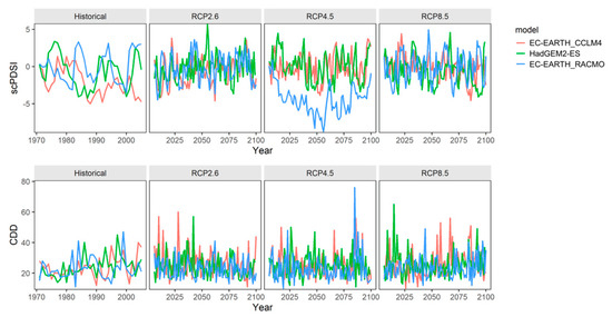
Figure 3.
Temporal variation of the self-calibrating Palmer Drought Severity Index (scPDSI) and maximum number of consecutive days with precipitation < 1 mm (CDD) indices considering historical and future scenarios (RCP2.6, RCP4.5, RCP8.5) calculated from daily precipitation data provided by the three GCMs (M1, M3, M4).
Regarding the timeframe of future changes in drought frequency, both the increase in scPDSI in RCP2.6 and the decrease detected in RCP8.5 would likely occur in the long-term timeframe, as reported in Table A5.
6.3. Wildfires
In the municipality of Trieste, median sFWi was ≈12 in the historical scenario for all the timeframes considered as presented in Figure 4, suggesting a moderate danger according to the EFFIS classification (Figure 5). Figure 5 represents the median number of days with moderate, high and very high fire danger conditions along the timeseries (median values of N15 = 41, N30 =14 and N45 = 4, respectively).
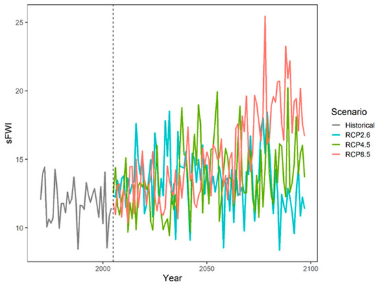
Figure 4.
Trend of seasonal Fire Weather Index (sFWI) for the municipality of Trieste. Grey line represents the historical scenario (1970–2004), while colored lines represent multi-model mean ensemble projections (2005–2097) based on three RCPs. Dashed line represents the starting year of the projections.
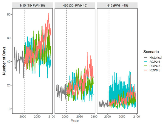
Figure 5.
Trend of the number of days with moderate (N15), high (N30) and very high (N45) fire danger conditions according to EFFIS classification. Grey line represents the historical scenario (1970–2004), while colored lines represent multi-model mean ensemble.
There is a significant increase both in hazard intensity and hazard frequency in RCP4.5 and RCP8.5, as reported in Table A6, while RCP2.6 did not show any significant trend, except for N45, where the negative slope observed is probably attributable to the high level of stochasticity in the projection (see blue line in Figure 5).
Table A7 reports the indicative timeframe in which a change is expected in the intensity/frequency of wildfires. Interestingly, all variables converged in estimating a significant potential change starting from a mid-term timeframe (2005–2066), except for N45, whose interpretation was described above.
6.4. Heatwaves and Cold Spells
The current incidence of heatwaves has been computed using data from a local weather station. Figure 6 shows the trend of heatwaves during the period between 1995 and 2019, and the critical periods in years 2003, 2006 and 2015 can be clearly seen. Figure 7 reports the distribution of cold spells and frost days in the historical period. Trieste is a rather warm city; therefore no CS are present, and the critical year appears to be 2012, characterized by a long, unusual period of low temperatures and strong wind from the northeast, called Bora, causing a consistent number of FD.
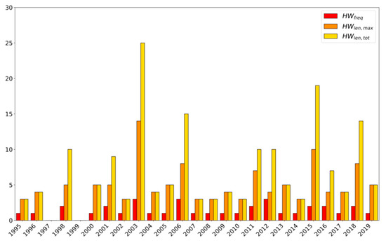
Figure 6.
Heatwaves in Trieste during 1995–2019 timeframe.
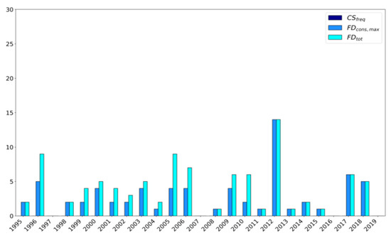
Figure 7.
Cold spell and frost day phenomena in Trieste during the 1995–2019 timeframe.
To compute the current probability of hazard, first, we calculated the fraction of the total amount of days included in heatwaves against the total number of days included in the summer months of June, July and August. Referring to the data measured at Trieste between 1995 and 2019, 173 days were included in heatwaves. Considering a total of 2300 summer days (92 per year for 25 years) for the analyzed timeframe, an occurrence percentage of 7.52% was obtained. This value is higher than the “extremely likely to happen” limit of 5%; therefore, the actual probability of these events is High.
In the same way, cold spell occurrences were computed. Because of the total absence of such phenomena in the 1995–2019 timeframe, the occurrence probability is 0%, and the actual probability of these events is Low.
By utilizing the projections of climate models, a study of the future evolution of extreme thermal events in Trieste was carried out. Due to the five models of Table 2 being applied to the three RCP scenarios, fifteen cases were considered; the availability of different models allowed us to take into account the uncertainty of the models. Therefore, the future evolution of heatwaves is here presented through boxplot graphs, presenting minimum, first quartile, median, third quartile and maximum, along with outliers. Through boxplots, data distribution characteristics can be quickly guessed, showing either data symmetry or how tightly the data is grouped.
Figure 8 presents the evolution of HWfreq up to the year 2100 for RCP 8.5; the boxplot collects the data obtained by applying the definition of HW to the five models considered. An inspection of Figure 8 highlights the increasing trend of heatwaves for a scenario as is, where no intervention for reducing dangerous emissions into the atmosphere has been developed.
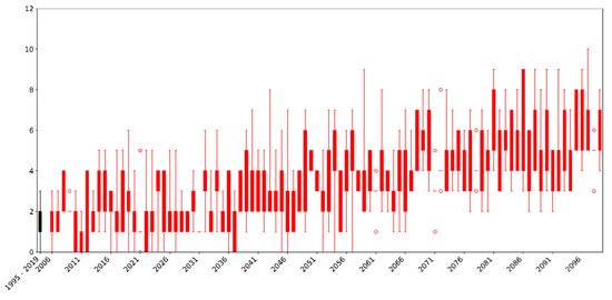
Figure 8.
Heatwave yearly frequency distribution for Trieste and the RCP8.5 scenario. Boxplot represent minimum, first quartile, third quartile, and maximum value. Distributions for the 2006–2100 timeframe were obtained through the five climatic models. Distribution for the historical timeframe, 1995–2019, is also reported in black color.
In order to obtain quantitative values to complete the CoM template, the modified Mann–Kendall trend test (MMKT) was applied to the frequency of events, computed as the total number of days included in extreme heat (cold) events compared to the total days of summer (winter) months.
For heatwave frequency, the test revealed statistically significant changes already in the 2020–2045 period for all cases except for the M4 model in the RCP4.5 scenario, which shows p = 0.06, as reported in Table A8. Heatwave intensity follows the same pattern, as it can also be deduced from the values of the Theil-Sen indicator in Table A9 where, again, only for the M4 model applied to RCP4.5, no change is identified. Consequently, for heatwaves, the choice for the expected frequency variation is the Increase option, while for the Timeframe, the choice is Short-Term. As regards cold spells, the test did not identify any statistically significant variation in the frequency of the phenomena in any of the periods analyzed for all combinations of climate models and RCP scenarios. Consequently, for cold spells, the choice regarding the frequency variation is the No Change option, while for the Timeframe, the choice falls on Long-Term.
The increasing trend in frequency and intensity suggests that mitigation and adaptation actions should be taken, since heat excess can have a significant impact on people’s health, especially vulnerable people [72,73]. Heatwaves in this paper were defined taking into account temperature only. However, other parameters are better suited for describing the effect of heat on people; for example, the Thom index [74] and Humidex [75] also take humidity into account and could be used to define heatwaves.
6.5. River Flood
For river floods, the proposed method for the completion of the SECAP template requires the presence of at least one risk level (from R1 to R4) according to Directive 2007/60/EC. Trieste is a one-of-a-kind city in terms of this natural hazard, as it lacks any significant river courses and can only be affected by hydraulic risk connected to coastal floods. Although the hazard risk analysis for river floods is not applicable to Trieste, it is worth furnishing some perspectives on future changes in the river flood regime in order to provide information useful to completing the CoM, at least at a regional level. Future changes in the river regimen will almost certainly be linked to rainfall. The trend of rainfall was evaluated in the most recent analysis by ARPA FVG [24]. The long-term (2071–2100) regional response to the RCP8.5 scenario foresees an increase in average and extreme precipitation, as well as in days of extreme precipitation in the winter, whereas in the summer, all three parameters will decrease. Considering the climate projections, it is highly probable that severe flood events will rise in number at a regional scale, even over short periods of time, unavoidably increasing the intensity and frequency of hazards and reducing the return periods of all the extremes. Regarding filling out the CoM template for the Trieste municipality, according to the above-mentioned reasons, the probability of flood hazard can be neglected, and it has been reported as “not known”.
6.6. Coastal Flood and Storm Surge
Figure 9 reports the results of the simulation for the scenario of +180 cm (above m.s.l.) flooding with a 30-year RP for the municipality of Trieste. The sum of the flooded areas amounts to 0.75 km2, unevenly distributed along the 30-km-long shoreline, but highly constrained by the topographic gradient, which limits the penetration. The majority of the inundation is concentrated in the city’s central portion, involving an area of 0.53 km2 of the historical center (including Borgo Teresiano and Piazza Unità d’Italia), which is exposed to a 2.2-km-long waterfront. Marine flooding penetrates up to 370 m toward the center, with a mean ingression of ca. 230 m.
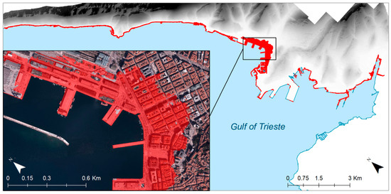
Figure 9.
Marine flooding scenario of the Trieste municipality, considering a 30-year return period of coastal flood (high tide + surge + set-up) of 180 cm above mean sea level (m.s.l.). In the box is a detail of the historical part of the city, including Borgo Teresiano and Piazza Unità d’Italia.
Considering the classification of the hazard, the level is High. The impact is also High, since inundation involves the most vulnerable historical part of the city. In November 2019, the phenomenon occurred almost twice, creating severe inconveniences to the population: a blockage in the main road network, damage to shops and interruption of electricity supply.
Hazard intensity and frequency are expected to increase in the future because of relative sea level rises. Considering a significant increase in sea level, starting from the mid-term timeframe, the 180-cm threshold will be exceeded more frequently, and a higher level will have an equal return period of 30 years, resulting in a greater extension of floodable areas. Therefore, all the extremes will reduce their RP.
6.7. Landslides
Figure 10 shows the distribution of landslides recorded in the municipality of Trieste, superimposed over the urban area classification.
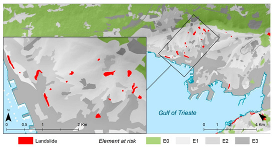
Figure 10.
Distribution of landslides recorded in the Trieste municipality. Landslides are superimposed over the urban area classification according to the four classes reported in Table 8.
The total number (N) of landslides recorded in the municipality of Trieste is 53, distributed in the territory of 85.11 km2. The corresponding ratio (N/km2) is 0.62.
According to the proposed classification of the level of hazard, reported in Table 9, the resulting level of hazard for Trieste is High. The impact of the hazard depends on the distribution of landslides that occur in every class of territory. Based on the precautionary principle, the impact of hazard is set to High.
It is reasonable to expect increased slope instability in the future and a subsequent increase in the number or extension of landslides as a result of an increase in short but intense precipitation episodes and/or an increase in cumulative precipitation (RX5day), infiltration and runoff [76]. As previously stated, the increasing trend will likely occur in the Long-Term timeframe (2071–2100). At any rate, much will depend on human action, thanks to monitoring, mitigation and safeguarding efforts.
7. Discussion
Filling out the CoM template is fundamental to identifying hazards and their evolution in time. In order to identify an existing hazard and its actual impact, municipalities can utilize databases of past events and the general knowledge at the site.
More problematic is how to project the data in a future timeframe. For rainfall and heat-related risks, the principal source of historical information is the database of measurements taken by weather stations directly on the site, or in nearby locations. Regional or local weather services are today widespread, and the information can be easily found. The problem with such data, however, stems from the fact that the timeseries of weather data can present missing or completely wrong values, so a data treatment should be performed for gap-filling and the removal of unfeasible data; alternatively, the historical simulation data can also be used. For future data, projections are obtained from international databases such as CORDEX [12]; it is advisable to use a minimum number of models and different RCP scenarios in order to account for the uncertainties intrinsic to the numerical methods. In this case, the retrieval of the data requires tools, freely available online, requiring an expertise usually not available in municipalities but that can be easily found in universities or research centers. In order to improve the data, techniques to correct bias errors are also encouraged. Once the data is obtained, the template can be filled by looking at the future behaviour, when appropriate metrics for the different hazards are on hand.
Table 12 reports selections for the analyzed hazards of Trieste, with each selection to be made when compiling the CoM template. The pattern followed in this paper allows a straightforward compilation once the defined parameters and their time evolution, according to the Mann–Kendall test, have been utilized in order to select the trend and the relative timeframe. It is worth noting that the use of statistical methods is of great importance when the trend is not clearly visible and the selection of a possible choice is not straightforward. In this case, this applies not only to “Heavy rainfall” and “Drought and water scarcity” where the “No change” option for changes of intensity or frequency are reported (Table A1 and Table A4), but also in the presence of clear trends that the analysis can discriminate with regard to the Timeframe under consideration. For instance, the analysis of Table 12 highlights the danger of increasing temperatures, with problems in the Short-Term and wildfire in the Mid-Term as consequences of the “Extreme heat” and “Drought and Water Scarcity” hazards. It is worth noting that the results obtained here are in line with the ones found by other authors; for example, a similar pattern was found in [15] for the municipality of San Donà di Piave, not far from Trieste.
Table 12.
CoM template for Trieste, (n.a. = not applicable).
Because of their unique nature, geological hazards have required a different approach. The most significant challenge in compiling the CoM template, in this case, was obtaining complete information from the municipality that wishes to participate in the program. It is difficult for a municipality to keep track of all landslide activation and reactivation events, for example. This means that there will be no frequency of occurrence and that the hazard and its impact will have to be parametrized in another way, presumably qualitatively or descriptively. In general, it is unlikely that each municipality will provide the same information needed for the compilation of the CoM template, making an approach for data manipulation difficult to generalize.
The proposed methods are an attempt to address these issues, through simplified procedures that require basic information which is easy to obtain or manipulate, such as standardized data for river flood risk, the number and extent of landslides and rockfalls in each territorial unit and the topography of the coastal area for the purposes of simulating marine inundation. To determine the probability of coastal floods and landslides, an analytical solution related to geographic distribution has been introduced, while for the future trend, the results pertaining to the cause-and effect relationship, linked to the intensity of “heavy rainfall” in a given timeframe, have been used for a simpler opinion (increase, decrease, no change, not known) on the expected trend.
8. Conclusions
This paper proposes a new approach to compiling the hazard part of the Covenant of Mayors’ Risk and Assessment template for creating SECAPs. In this case, the method was applied to the municipality of Trieste in northern Italy. The proposed method combines data available in local weather databases and future projections from GCM-RCM simulations. Different hazards were considered: specifically, those related to rain, temperature and geological movements. For each identified hazard, first, some parameters were identified in order to numerically describe their frequency and intensity; then, the parameters were used to identify actual probability and future behavior. When dealing with the future projection of each hazard, the method proposed here utilizes the Mann–Kendall test in order to identify the trend. The method proved to be a useful technique that can provide the required information needed to fill out the template. The proposed method uses a statistical approach to support the inserted values rather than relying solely on a heuristic method based on the “experience” of the person in charge of filling out the template.
The availability of historical data, which may be incomplete and the method for manipulating future climatic data projections are identified as problems for the application of the proposed method. Certain types of expertise are not always available in municipalities, necessitating the use of an external support system or network. Again, the simplified approach used to quantify geological hazards is reliant on data available at the municipal level, though topographical details, as well as information on floods and landslides, are becoming more readily available and accessible.
This is a first attempt to define a procedure for assisting administrations in participating in the CoM initiative, made possible by the collaboration of the municipality of Trieste, where a general increase in the intensity and frequency of hazards can be identified. Future development could include expanding to other municipalities or provinces within a region, as well as collaborating with neighboring countries.
Author Contributions
Conceptualization, M.M., G.B., A.N. and G.F.; methodology, M.M., G.B., A.N., G.F., G.C., A.P., E.T. and F.P.; software, G.C., A.P., E.T. and F.P.; validation, G.C, A.P., E.T. and F.P.; formal analysis, A.P., E.T., F.P. and G.C.; data curation, G.C., A.P., E.T. and F.P.; writing—original draft preparation, M.M.; writing—review and editing, M.M., G.B., A.N., G.F., G.C., A.P., E.T. and F.P.; visualization, G.C., A.P., E.T. and F.P.; supervision, M.M., G.B., A.N. and G.F.; project administration, M.M.; funding acquisition, M.M., A.N., G.F. and G.B. All authors have read and agreed to the published version of the manuscript.
Funding
This research was funded by EU Interreg Italia–Slovenja project SECAP, OS 2.1, PI 4e, https://www.ita-slo.eu/it/secap (accessed on 4 April 2022).
Data Availability Statement
Publicly available datasets were analyzed in this study. This data can be found here: [https://www.osmer.fvg.it/clima.php?ln=] (accessed on 4 April 2022).
Acknowledgments
The help of the Regional Agency for the Protection of the Environment, ARPA FVG, is gratefully acknowledged.
Conflicts of Interest
The authors declare no conflict of interest.
Appendix A
Table A1.
Summary of modified Mann–Kendall trend tests and Sen’s slope and associated confidence intervals (C.I.) of the number of days with precipitation > 20 mm (R20mm) and maximum five-day precipitation (RX5day). Indices were computed considering historical and future scenarios (RCP2.6, RCP4.5, RCP8.5) calculated from daily precipitation data provided by the three GCMs (EC-EARTH_CCLM4, HadGEM2-ES, EC-EARTH_RACMO) for the City of Trieste. Bold numbers = statistically significant modified Mann–Kendall trend test and slope values (α = 0.05).
| Climatic Index | Historical | RCP2.6 | RCP4.5 | RCP8.5 | ||||
|---|---|---|---|---|---|---|---|---|
| Slope | C.I. | Slope | C.I. | Slope | C.I. | Slope | C.I. | |
| R20mm | ||||||||
| M3 | 0.00 | −0.17; 0.15 | 0.03 | 0.00; 0.08 | 0.00 | −0.03; 0.04 | 0.00 | −0.02; 0.05 |
| M1 | 0.00 | −0.18; 0.17 | 0.02 | 0.00; 0.06 | −0.02 | −0.07; 0.01 | 0.00 | −0.01; 0.04 |
| M4 | 0.00 | −0.14; 0.19 | 0.00 | −0.02; 0.04 | 0.02 | 0.00; 0.06 | 0.03 | 0.00; 0.07 |
| RX5day | ||||||||
| M3 | −0.20 | −1.02; 0.68 | 0.13 | −0.08; 0.34 | 0.08 | −0.13; 0.31 | 0.29 | 0.10; 0.57 |
| M1 | 0.20 | −0.83; 1.12 | 0.24 | 0.01; 0.44 | −0.06 | −0.31; 0.18 | 0.25 | 0.01; 0.45 |
| M4 | 0.43 | −0.64; 1.19 | −0.06 | −0.24; 0.14 | 0.04 | −0.14; 0.21 | 0.21 | −0.01; 0.43 |
Table A2.
Indicative timeframe in which a change is expected in heavy precipitation intensity (RX5day) for each model and for each scenario. Values represent Sen’s slope of timeseries having significance and Mann-Kendall trend test (p < 0.05) calculated within each time window. Short-Term = 2020–2045; Mid-Term = 2046–2070; Long-Term = 2071–2100. n.s. = Not Significant.
| RX5day (RCP8.5) | Short-Term | Mid-Term | Long-Term |
|---|---|---|---|
| M3 | n.s. | n.s. | 0.29 |
| M1 | n.s. | n.s. | 0.25 |
| M4 | n.s. | n.s. | 0.21 |
Table A3.
Drought classes based on scPDSI values.
Table A3.
Drought classes based on scPDSI values.
| scPDSI | Drought Class |
|---|---|
| ≥4.00 | Extreme wet |
| 3.00~3.99 | Severe wet |
| 2.00~2.99 | Moderate wet |
| 1.00~1.99 | Mild wet |
| −0.99~0.99 | Normal |
| −1.99~−1.00 | Mild drought |
| −2.99~−2.00 | Moderate drought |
| −3.99~−3.00 | Severe drought |
| ≤−4.00 | Extreme drought |
Table A4.
Summary of modified Mann–Kendall trend tests and Sen’s slope as well as associated confidence intervals (C.I.) of self-calibrating Palmer Drought Severity Index (scPDSI) and maximum number of consecutive days with precipitation < 1 mm (CDD). Indices computed by considering historical and future scenarios (RCP2.6, RCP4.5, RCP8.5) calculated from daily precipitation data provided by the three GCMs (HadGEM2-ES, EC-EARTH_CCLM4, EC-EARTH_RACMO) for the City of Trieste. Bold numbers = statistically significant modified Mann–Kendall trend tests and slope values (α = 0.05).
| Climatic index | Historical | RCP2.6 | RCP4.5 | RCP8.5 | ||||
|---|---|---|---|---|---|---|---|---|
| Slope | C.I. | Slope | C.I. | Slope | C.I. | Slope | C.I. | |
| scPDSI | ||||||||
| M3 | −0.10 | −0.16; −0.04 | 0.02 | 0.01; 0.04 | 0.01 | −0.01; 0.01 | −0.02 | −0.03; −0.01 |
| M1 | −0.04 | −0.13; 0.05 | 0.02 | 0.01; 0.03 | −0.01 | −0.03; 0.01 | −0.02 | −0.03; −0.01 |
| M4 | 0.03 | −0.07; 0.10 | 0.01 | −0.01; 0.02 | −0.01 | −0.03; 0.01 | 0.01 | −0.01; 0.02 |
| CDD | ||||||||
| M3 | 0.19 | −0.07; 0.45 | −0.02 | −0.08; 0.03 | −0.03 | −0.08; 0.02 | 0.06 | 0.00; 0.13 |
| M1 | 0.30 | 0.12; 0.44 | −0.05 | −0.09; 0 | 0.00 | −0.06; 0.05 | 0.03 | −0.02; 0.09 |
| M4 | 0.04 | −0.15; 0.25 | −0.02 | −0.07; 0.01 | −0.02 | −0.06; 0.03 | 0.00 | −0.04; 0.06 |
Table A5.
Indicative timeframe in which a change is expected in the self-calibrating Palmer Drought Severity Index (scPDSI) for each model and for each scenario. Values represent Sen’s slope of timeseries having significance and Mann–Kendall trend test (p < 0.05) calculated within each time 0window. Short-term = 2020–2045; Mid-term = 2046–2070; Long-term = 2071–2100. n.s. = Not Significant.
| Short-Term | Mid-Term | Long-Term | |
|---|---|---|---|
| scPDSI (RCP2.6) | |||
| M3 | n.s. | n.s. | 0.02 |
| M1 | n.s. | 0.06 | 0.01 |
| M4 | n.s. | n.s. | n.s. |
| scPDSI (RCP8.5) | |||
| M3 | n.s. | n.s. | −0.02 |
| M1 | n.s. | n.s. | −0.02 |
| M4 | n.s. | n.s. | n.s. |
Table A6.
Sen’s slope and related 95% confidence intervals for each index and each scenario. Bold values represent significant outcomes (p < 0.05) of Mann–Kendall trend Test.
Table A6.
Sen’s slope and related 95% confidence intervals for each index and each scenario. Bold values represent significant outcomes (p < 0.05) of Mann–Kendall trend Test.
| Variable | Scenario | Sen’s Slope | 95% C.I. |
|---|---|---|---|
| sFWI | Historical | −0.01 | −0.06; 0.05 |
| RCP2.6 | −0.01 | −0.03; 0.00 | |
| RCP4.5 | 0.03 | 0.01; 0.05 | |
| RCP8.5 | 0.09 | 0.07; 0.10 | |
| N15 | Historical | 0.00 | −0.22; 0.22 |
| RCP2.6 | −0.05 | −0.12; 0.00 | |
| RCP4.5 | 0.11 | 0.04; 0.17 | |
| RCP8.5 | 0.32 | 0.26; 0.38 | |
| N30 | Historical | −0.04 | −0.17; 0.10 |
| RCP2.6 | −0.04 | −0.08; 0.00 | |
| RCP4.5 | 0.08 | 0.04; 0.13 | |
| RCP8.5 | 0.21 | 0.17; 0.26 | |
| N45 | Historical | 0.00 | −0.07; 0.03 |
| RCP2.6 | −0.11 | −0.13; −0.10 | |
| RCP4.5 | 0.03 | 0.00; 0.06 | |
| RCP8.5 | 0.10 | 0.08; 0.13 |
Table A7.
Indicative timeframe in which a change is expected in intensity/frequency of the hazard for each variable and for each scenario. Values represent Sen’s slope of timeseries having significance and Mann–Kendall trend test (p < 0.05) calculated within each time window. Short-term = 2020–2045; Mid-term = 2046–2070; Long-term = 2071–2100. n.s. = Not Significant.
| Variable | Scenario | Short-Term | Mid-Term | Long-Term |
|---|---|---|---|---|
| sFWI | RCP2.6 | n.s. | −0.05 | n.s. |
| RCP4.5 | n.s. | 0.06 | 0.03 | |
| RCP8.5 | n.s. | 0.05 | 0.09 | |
| N15 | RCP2.6 | n.s. | n.s. | n.s. |
| RCP4.5 | n.s. | 0.20 | 0.11 | |
| RCP8.5 | n.s. | 0.20 | 0.32 | |
| N30 | RCP2.6 | n.s. | n.s. | n.s. |
| RCP4.5 | n.s. | 0.14 | 0.08 | |
| RCP8.5 | n.s. | 0.10 | 0.21 | |
| N45 | RCP2.6 | −0.28 | −0.16 | −0.11 |
| RCP4.5 | n.s. | 0.06 | 0.03 | |
| RCP8.5 | n.s. | 0.03 | 0.10 |
Table A8.
Modified Mann–Kendall test results for heatwave frequency for 2020–2045 timeframe.
Table A8.
Modified Mann–Kendall test results for heatwave frequency for 2020–2045 timeframe.
| RCP2.6 | RCP4.5 | RCP8.5 | ||||
|---|---|---|---|---|---|---|
| Trend | T.S. | Trend | T.S. | Trend | T.S. | |
| M1 | Increase | 0.18 | Increase | 0.18 | Increase | 0.18 |
| M2 | Increase | 0.32 | Increase | 0.57 | Increase | 0.58 |
| M3 | Increase | 0.18 | Increase | 0.19 | Increase | 0.17 |
| M4 | Increase | 0.17 | No Change | 0.06 | Increase | 0.28 |
| M5 | Increase | 0,35 | Increase | 0.26 | Increase | 0.37 |
Table A9.
Modified Mann–Kendall test results for heatwave intensity for 2020–2045 timeframe.
Table A9.
Modified Mann–Kendall test results for heatwave intensity for 2020–2045 timeframe.
| RCP2.6 | RCP4.5 | RCP8.5 | ||||
|---|---|---|---|---|---|---|
| Trend | T.S. | Trend | T.S. | Trend | T.S. | |
| M1 | Increase | 0.09 | Increase | 0.11 | Increase | 0.08 |
| M2 | Increase | 0.10 | Increase | 0.21 | Increase | 0.20 |
| M3 | Increase | 0.07 | Increase | 0.07 | Increase | 0.05 |
| M4 | Increase | 0.08 | No Change | 0.00 | Increase | 0.12 |
| M5 | Increase | 0.16 | Increase | 0.11 | No Change | 0.19 |
Appendix B
The statistical analysis of data from the FVG Regional Cadaster of Landslides covers 116 out of 215 municipalities in Friuli Venezia Giulia. The Cadaster is also available as WebGIS [77], with 5726 landslides and rockfalls recorded.
We calculated the statistics of municipalities with a given number of landslides (N) to define a hazard scale available for the entire region and applicable to a specific municipality (Figure A1a). The statistics have also been referred to as the number of landslides normalized to the municipality’s surface area (Figure A1b).

Figure A1.
Statistics of the number of landslides (a) and number of landslides per km2 (b) occurring in the 116 municipalities of the FVG Region.
In this way, the magnitude and intensity of the landslide phenomenon can be determined. Using both parameters, testing their correlation and limiting the field of existence, a ranking on the CoM scheme’s Low–Moderate–High hazard scale was obtained (Figure A2).
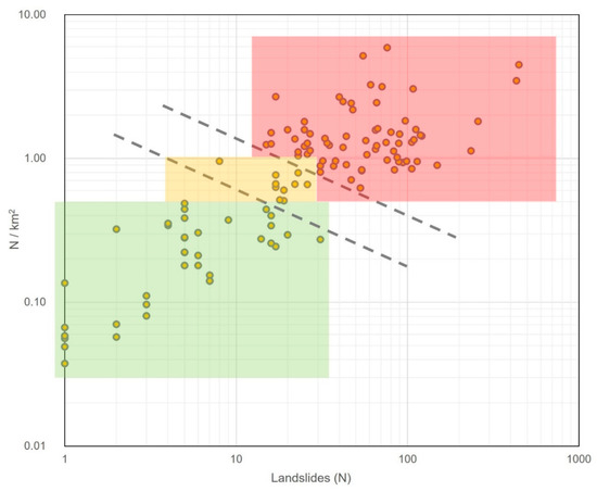
Figure A2.
Correlation between number of landslides (N) and number of landslides per km2 occurring in the 116 municipalities of the FVG Region. The rectangles include the three levels of hazard (by color) separated by the dashed lines. See Table 9 for the final ranking.
There are at least two conclusions that can be made based on Figure A2. The first is that, when trying to imagine what it means to have a landslide per square kilometer, the magnitude of criticality can be quickly realized. As a result, the value N/km2 = 1 can be considered to be the critical value, above which, the risk is high. The second is to look for an “outlier” that is less than 1 N/km2 in order to pinpoint an area where the hazard is low. The point with the coordinates N = 31 and N/km2 = 0.27 was thought to be plausible. Given the logarithmic scale of the axes and the preceding considerations, two half-lines were drawn to identify the hazard classification bands, taking both the values N and N/km2 into account (see Table 9).
References
- Synthesis Report—IPCC. Available online: https://www.ipcc.ch/ar6-syr/ (accessed on 3 January 2022).
- IPCC. Intergovermental Panel on Climate Change. In Proceedings of the AR6 Scoping Meeting, Addis Abeba, Ethiopia, 1–5 May 2017. [Google Scholar]
- Maragno, D.; Dall’Omo, C.F.; Ruzzante, F.; Musco, F. Toward a trans-regional vulnerability assessment for Alps. A methodological approach to land cover changes over alpine landscapes, supporting urban adaptation. Urban Clim. 2020, 32, 100622. [Google Scholar] [CrossRef]
- European Commission. The Europen Green Deal. Available online: https://ec.europa.eu/info/sites/default/files/european-green-deal-communication_en.pdf (accessed on 23 December 2021).
- Rivas, S.; Urraca, R.; Palermo, V.; Bertoldi, P. Covenant of Mayors 2020: Drivers and Barriers for Monitoring Climate Action Plans. J. Clean. Prod. 2022, 332, 130029. [Google Scholar] [CrossRef]
- Kamenders, A.; Rosa, M.; Kass, K. Low carbon municipalities. The impact of energy management on climate mitigation at local scale. Energy Procedia 2017, 128, 172–178. [Google Scholar] [CrossRef]
- Pablo-Romero, M.P.; Sánchez-Braza, A.; González-Limón, J.M. Covenant of Mayors: Reasons for Being an Environmentally and Energy Friendly Municipality. Rev. Policy Res. 2015, 32, 576–599. [Google Scholar] [CrossRef]
- Kona, A.; Bertoldi, P.; Monforti-Ferrario, F.; Rivas, S.; Dallemand, J.F. Covenant of mayors signatories leading the way towards 1.5 degree global warming pathway. Sustain. Cities Soc. 2018, 41, 568–575. [Google Scholar] [CrossRef]
- Pietrapertosa, F.; Salvia, M.; De Gregorio Hurtado, S.; D’Alonzo, V.; Church, J.M.; Geneletti, D.; Musco, F.; Reckien, D. Urban climate change mitigation and adaptation planning: Are Italian cities ready? Cities 2019, 91, 93–105. [Google Scholar] [CrossRef]
- Jekabsone, A.; Marín, J.P.D.; Martins, S.; Rosa, M.; Kamenders, U. Upgrade from SEAP to SECAP: Experience of 6 European Municipalities. Environ. Clim. Technol. 2021, 25, 254–264. [Google Scholar] [CrossRef]
- Publications Office of the the European Union. Guidebook “How to Develop a Sustainable Energy and Climate Action Plan (SECAP)”. Part 2, Baseline Emission Inventory (BEI) and Risk and Vulnerability Assessment (RVA). Available online: https://op.europa.eu/en/publication-detail/-/publication/a2ac8a5e-f134-11e8-9982-01aa75ed71a1/language-en (accessed on 21 April 2022).
- EURO-CORDEX. Available online: https://www.euro-cordex.net/ (accessed on 5 January 2022).
- Report on Climate Analysis and Vulnerability Assessment Results in the Pilot Region (Sardinia Region) and in the Areas Targeted in Action C3. Available online: https://masteradapt.eu/wordpress/wp-content/uploads/2017/09/MA-report-A1.pdf (accessed on 28 March 2022).
- Hamed, K.H.; Ramachandra Rao, A. A Modified Mann-Kendall Trend Test for Autocorrelated Data. J. Hydrol. 1998, 204, 182–196. [Google Scholar] [CrossRef]
- Magni, F.; Musco, F.; Litt, G.; Carraretto, G. The Mainstreaming of Nbs in the Secap of San Donà Di Piave: The Life Master Adapt Methodology. Sustainability 2020, 12, 80. [Google Scholar] [CrossRef]
- Brownlee, T.D.; Camaioni, C.; Magaudda, S.; Mugnoz, S.; Pellegrino, P. The INTERREG Italy-Croatia Joint_SECAP Project: A Collaborative Approach for Adaptation Planning. Sustainability 2021, 14, 404. [Google Scholar] [CrossRef]
- Vlachogiannis, D.; Sfetsos, A.; Markantonis, I.; Politi, N.; Karozis, S.; Gounaris, N. Quantifying the Occurrence of Multi-Hazards Due to Climate Change. Appl. Sci. 2022, 12, 1218. [Google Scholar] [CrossRef]
- Ilori, O.W.; Ajayi, V.O. Change Detection and Trend Analysis of Future Temperature and Rainfall over West Africa. Earth Syst. Environ. 2020, 4, 493–512. [Google Scholar] [CrossRef]
- SECAP. Italia Slovenia. Available online: https://www.ita-slo.eu/it/secap (accessed on 28 March 2022).
- The Covenant of Mayors Reporting Templates. Available online: http://com-east.eu/en/faq-3/itemlist/category/227-the-covenant-of-mayors-reporting-templates/ (accessed on 5 January 2022).
- Chokkavarapu, N.; Mandla, V.R. Comparative study of GCMs, RCMs, downscaling and hydrological models: A review toward future climate change impact estimation. SN Appl. Sci. 2019, 1, 1698. [Google Scholar] [CrossRef] [Green Version]
- Machard, A.; Inard, C.; Alessandrini, J.-M.; Pelé, C.; Ribéron, J. A Methodology for Assembling Future Weather Files Including Heatwaves for Building Thermal Simulations from the European Coordinated Regional Downscaling Experiment (EURO-CORDEX) Climate Data. Energies 2020, 13, 3424. [Google Scholar] [CrossRef]
- The Covenant of Mayors for Climate and Energy Reporting Guidelines. Available online: https://www.covenantofmayors.eu/IMG/pdf/Covenant_ReportingGuidelines.pdf (accessed on 13 January 2022).
- Arpa FVG. Studio Conoscitivo Dei Cambiamenti Climatici e Di Alcuni Loro Impatti in Friuli Venezia Giulia. 2018. Available online: https://www.meteo.fvg.it/clima/clima_fvg/03_cambiamenti_climatici/01_REPORT_cambiamenti_climatici_e_impatti_per_il_FVG/impattiCCinFVG_marzo2018.pdf (accessed on 28 March 2022).
- Hu, C.; Xu, Y.; Han, L.; Yang, L.; Xu, G. Long-Term Trends in Daily Precipitation over the Yangtze River Delta Region during 1960–2012, Eastern China. Theor. Appl. Climatol. 2016, 125, 131–147. [Google Scholar] [CrossRef]
- Su, L.; Li, J.; Shi, X.; Fung, J.C.H. Spatiotemporal Variation in Presummer Precipitation over South China from 1979 to 2015 and Its Relationship with Urbanization. J. Geophys. Res. Atmos. 2019, 124, 6737–6749. [Google Scholar] [CrossRef]
- Sharma, S.; Khadka, N.; Hamal, K.; Shrestha, D.; Talchabhadel, R.; Chen, Y. How Accurately Can Satellite Products (TMPA and IMERG) Detect Precipitation Patterns, Extremities, and Drought Across the Nepalese Himalaya? Earth Space Sci. 2020, 7, e2020EA001315. [Google Scholar] [CrossRef]
- Bronaugh, D. Climdex.Pcic: PCIC Implementation of Climdex Routines Version 1.1-11 from CRAN. Available online: https://rdrr.io/cran/climdex.pcic/ (accessed on 1 April 2022).
- Wells, N.; Goddard, S.; Hayes, M.J. A Self-Calibrating Palmer Drought Severity Index. J. Clim. 2004, 17, 2335–2351. [Google Scholar] [CrossRef]
- Tian-Jun, Z.; Tao, H. Projected Changes of Palmer Drought Severity Index under an RCP8.5 Scenario. Atmos. Ocean. Sci. Lett. 2013, 6, 273–278. [Google Scholar] [CrossRef]
- Dubrovský, M.; Hayes, M.; Duce, P.; Trnka, M.; Svoboda, M.; Zara, P. Multi-GCM projections of future drought and climate variability indicators for the Mediterranean region. Reg. Environ. Chang. 2013, 14, 1907–1919. [Google Scholar] [CrossRef]
- Van Der Schrier, G.; Briffa, K.; Jones, P.D.; Osborn, T. Summer Moisture Variability across Europe. J. Clim. 2006, 19, 2818–2834. [Google Scholar] [CrossRef]
- Duan, Y.; Ma, Z.; Yang, Q. Characteristics of Consecutive Dry Days Variations in China. Theor. Appl. Climatol. 2017, 130, 701–709. [Google Scholar] [CrossRef] [Green Version]
- Hargreaves, G.H. Defining and Using Reference Evapotranspiration. J. Irrig. Drain. Eng. 1994, 120, 1132–1139. [Google Scholar] [CrossRef]
- Droogers, P.; Allen, R.G. Estimating Reference Evapotranspiration Under Inaccurate Data Conditions. Irrig. Drain. Syst. 2002, 16, 33–45. [Google Scholar] [CrossRef]
- Beguería, S.; Vicente-Serrano, S.M.; Reig, F.; Latorre, B. Standardized precipitation evapotranspiration index (SPEI) revisited: Parameter fitting, evapotranspiration models, tools, datasets and drought monitoring. Int. J. Clim. 2014, 34, 3001–3023. [Google Scholar] [CrossRef] [Green Version]
- ScPDSI: Calculation of the Conventional and Self-Calibrating Palmer Drought Severity Index Version 0.1.3 from CRAN. Available online: https://rdrr.io/cran/scPDSI/ (accessed on 1 April 2022).
- Hobday, A.J.; Alexander, L.V.; Perkins, S.E.; Smale, D.A.; Straub, S.C.; Oliver, E.C.J.; Benthuysen, J.A.; Burrows, M.T.; Donat, M.G.; Feng, M.; et al. A hierarchical approach to defining marine heatwaves. Prog. Oceanogr. 2016, 141, 227–238. [Google Scholar] [CrossRef] [Green Version]
- Van Wagner, C.E. Development and Structure of the Canadian Forest Fire Weather Index System; Canadian Forest Service Publications: Ottawa, ON, Canada, 1987; ISBN 0662151984. [Google Scholar]
- EFFIS. Welcome to EFFIS. Available online: https://effis.jrc.ec.europa.eu/ (accessed on 3 April 2022).
- Copernicus Database. Available online: https://cds.climate.copernicus.eu/#!/home (accessed on 3 April 2022).
- Giannakopoulos, C.; Karali, A. Fire Weather Index (FWI)—Dataset Description. Copernicus Climate Change Service. Available online: https://datastore.copernicus-climate.eu/documents/sis-european-tourism/C3S_D422_Lot2_TEC_FWI_dataset_description_v1.1.pdf (accessed on 1 April 2022).
- Agbazo, M.N.; Grenier, P. Characterizing and Avoiding Physical Inconsistency Generated by the Application of Univariate Quantile Mapping on Daily Minimum and Maximum Temperatures over Hudson Bay. Int. J. Climatol. 2020, 40, 3868–3884. [Google Scholar] [CrossRef]
- Grenier, P. Two Types of Physical Inconsistency to Avoid with Univariate Quantile Mapping: A Case Study over North America Concerning Relative Humidity and Its Parent Variables. J. Appl. Meteorol. Climatol. 2018, 57, 347–364. [Google Scholar] [CrossRef]
- Thrasher, B.; Maurer, E.P.; McKellar, C.; Duffy, P.B. Technical Note: Bias Correcting Climate Model Simulated Daily Temperature Extremes with Quantile Mapping. Hydrol. Earth Syst. Sci. 2012, 16, 3309–3314. [Google Scholar] [CrossRef] [Green Version]
- Cannon, A.J.; Sobie, S.R.; Murdock, T.Q. Bias Correction of GCM Precipitation by Quantile Mapping: How Well Do Methods Preserve Changes in Quantiles and Extremes? J. Clim. 2015, 28, 6938–6959. [Google Scholar] [CrossRef]
- Casati, B.; Yagouti, A.; Chaumont, D. Regional Climate Projections of Extreme Heat Events in Nine Pilot Canadian Communities for Public Health Planning. J. Appl. Meteorol. Clim. 2013, 52, 2669–2698. [Google Scholar] [CrossRef]
- Robinson, P.J. On the Definition of a Heat Wave; American Meteorological Society: Boston, MA, USA, 2001; Volume 40. [Google Scholar]
- Logan, T.; Bourgault, P.; Smith, T.J.; Huard, D.; Biner, S.; Labonté, M.-P.; Rondeau-Genesse, G.; Fyke, J.; Aoun, A.; Roy, P.; et al. Ouranosinc/Xclim, V0.31.0; Zenoob: Vancouver, BC, Canada, 2021. [Google Scholar] [CrossRef]
- Diffenbaugh, N.S.; Field, C.B. Changes in Ecologically Critical Terrestrial Climate Conditions. Science 2013, 341, 486–492. [Google Scholar] [CrossRef] [PubMed] [Green Version]
- Lopresti, A.; Charland, A.; Woodard, D.; Randerson, J.; Diffenbaugh, N.S.; Davis, S.J. Rate and velocity of climate change caused by cumulative carbon emissions. Environ. Res. Lett. 2015, 10, 095001. [Google Scholar] [CrossRef]
- Gariano, S.L.; Guzzetti, F. Landslides in a changing climate. Earth Sci. Rev. 2016, 162, 227–252. [Google Scholar] [CrossRef] [Green Version]
- Crozier, M.J. Deciphering the effect of climate change on landslide activity: A review. Geomorphology 2010, 124, 260–267. [Google Scholar] [CrossRef]
- Vousdoukas, M.; Mentaschi, L.; Mongelli, I.; Ciscar Martinez, J.C.; Hinkel, J.; Ward, P.; Gosling, S.; Feyen, L. Adapting to Rising Coastal Flood Risk in the EU under Climate Change; Publications Office of the the European Union: Luxembourg, 2020. [Google Scholar] [CrossRef]
- Ramieri, E.; Hartley, A.J.; Barbanti, A.; Santos, F.D.; Gomes, A.; Hilden, M.; Laihonen, P.; Marinova, N.; Santini, M. Methods for Assessing Coastal Vulnerability to Climate Change. In European Topic Centre on Climate Change Impacts, Vulnerability and Adaptation; European Environment Agency: Copenhagen, Denmark, 2011; pp. 1–93. [Google Scholar]
- Kuhn, M.; Tuladhar, D.; Corner, R. Visualising the Spatial Extent of Predicted Coastal Zone Inundation Due to Sea Level Rise in South-West Western Australia. Ocean. Coast. Manag. 2011, 54, 796–806. [Google Scholar] [CrossRef]
- EEA. Climate Change Adaptation and Disaster Risk Reduction in Europe. Enhancing Coherence of the Knowledge Base, Policies and Practices; European Enviroment Agency: Copenhagen, Denmark, 2017; ISBN 9780874216561. [Google Scholar]
- Dottori, F.; Mentaschi, L.; Bianchi, A.; Alfieri, L.; Feyen, L. JRC Technical Report. Adapting to Rising River Flood Risk in the EU under Climate Change JRC PESETA IV Project-Task 5; JRC Publications Repository: Schagen, The Netherlands, 2020; ISBN 978-92-76-12946-2. [Google Scholar]
- Castellari, S.; Venturini, S.; Ballarin Denti, A.; Bigano, A.; Bindi, M.; Bosello, F.; Carrera, L.; Chiriaco, M.V.; Danovaro, R.; Desiato, F.; et al. Rapporto Sullo Stato Delle Conoscenze Scientifiche Su Impatti, Vulnerabilità Ed Adattamento Ai Cambiamenti Climatici in Italia; Ministero dell’Ambiente e della Tutela del Territorio e del Mare: Roma, Italy, 2014; ISBN 9788887728095. [Google Scholar]
- Purvis, M.J.; Bates, P.D.; Hayes, C.M. A Probabilistic Methodology to Estimate Future Coastal Flood Risk Due to Sea Level Rise. Coast. Eng. 2008, 55, 1062–1073. [Google Scholar] [CrossRef]
- Distretto Idrografico Delle Alpi Orientali. Piano Di Gestione Del Rischio Alluvioni (Flood Risk Management Plan)—Relazione Di Piano e Allegati. Available online: http://www.alpiorientali.it/dati/direttive/alluvioni/fd_20160309/PGRA_Relazione di Piano_Allegati_I_II_III_V.pdf (accessed on 4 April 2022).
- Friuli Venezia Giulia Autonomous Region—Enviromental and Territorial Data Catalogue—IRDATfvg—Dettaglio-Diretto. Available online: https://irdat.regione.fvg.it/consultatore-dati-ambientali-territoriali/detail/irdat/dataset/1787 (accessed on 3 April 2022).
- Antonioli, F.; Anzidei, M.; Amorosi, A.; Lo Presti, V.; Mastronuzzi, G.; Deiana, G.; De Falco, G.; Fontana, A.; Fontolan, G.; Lisco, S.; et al. Sea-Level Rise and Potential Drowning of the Italian Coastal Plains: Flooding Risk Scenarios for 2100. Quat. Sci. Rev. 2017, 158, 29–43. [Google Scholar] [CrossRef] [Green Version]
- Marsico, A.; Lisco, S.; Lo Presti, V.; Antonioli, F.; Amorosi, A.; Anzidei, M.; Deiana, G.; De Falco, G.; Fontana, A.; Fontolan, G.; et al. Flooding Scenario for Four Italian Coastal Plains Using Three Relative Sea Level Rise Models. J. Maps 2017, 13, 961–967. [Google Scholar] [CrossRef] [Green Version]
- Bonaldo, D.; Antonioli, F.; Archetti, R.; Bezzi, A.; Correggiari, A.; Davolio, S.; De Falco, G.; Fantini, M.; Fontolan, G.; Furlani, S.; et al. Integrating multidisciplinary instruments for assessing coastal vulnerability to erosion and sea level rise: Lessons and challenges from the Adriatic Sea, Italy. J. Coast. Conserv. 2019, 23, 19–37. [Google Scholar] [CrossRef]
- Cruden, D.M.; Varnes, D.J. Landslide Types and Processes; Special Report, Transportation; U.S. National Academy of Sciences: Washington, DC, USA, 1996. [Google Scholar]
- Alvioli, M.; Melillo, M.; Guzzetti, F.; Rossi, M.; Palazzi, E.; von Hardenberg, J.; Brunetti, M.T.; Peruccacci, S. Implications of Climate Change on Landslide Hazard in Central Italy. Sci. Total Environ. 2018, 630, 1528–1543. [Google Scholar] [CrossRef] [PubMed]
- Guzzetti, F.; Carrara, A.; Cardinali, M.; Reichenbach, P. Landslide Hazard Evaluation: A Review of Current Techniques and Their Application in a Multi-Scale Study, Central Italy. Geomorphology 1999, 31, 181–216. [Google Scholar] [CrossRef]
- The, A.; Basin, R. On Integrating Climate Change Projection Into Landslide Risk Assessments & Mapping; The Association of Southeast Asian Nations (ASEAN): Jakarta, Indonesia, 2021; ISBN 9786236945148. [Google Scholar]
- Argyriou, A.V.; Polykretis, C.; Teeuw, R.M.; Papadopoulos, N. Geoinformatic Analysis of Rainfall-Triggered Landslides in Crete (Greece) Based on Spatial Detection and Hazard Mapping. Sustainability 2022, 14, 3956. [Google Scholar] [CrossRef]
- Crosta, G.B.; Frattini, P. Distributed modelling of shallow landslides triggered by intense rainfall. Nat. Hazards Earth Syst. Sci. 2003, 3, 81–93. [Google Scholar] [CrossRef] [Green Version]
- Nairn, J.R.; Fawcett, R.J.B. The Excess Heat Factor: A Metric for Heatwave Intensity and Its Use in Classifying Heatwave Severity. Int. J. Environ. Res. Public Health 2014, 12, 227–253. [Google Scholar] [CrossRef] [Green Version]
- Nairn, J.; Ostendorf, B.; Bi, P. Performance of Excess Heat Factor Severity as a Global Heatwave Health Impact Index. Int. J. Environ. Res. Public Health 2018, 15, 2494. [Google Scholar] [CrossRef] [Green Version]
- Epstein, Y.; Moran, D.S. Thermal Comfort and the Heat Stress Indices. Ind. Health 2006, 44, 388–398. [Google Scholar] [CrossRef] [Green Version]
- Masterton, J. Humidex a Method of Quantifying Human Discomfort Due to Excessive Heat and Humidity; Environment Canada Atmospheric Environment: Toronto, ON, Canada, 1979. [Google Scholar]
- Borgatti, L.; Soldati, M. Hillslope Processes and Climate Change. In Treatise on Geomorphology; Elsevier Inc.: Amsterdam, The Netherlands, 2013; Volume 7, pp. 306–319. ISBN 9780080885223. [Google Scholar]
- EagleFVG—Sistema Di Consultazione Delle Banche Dati Territoriali Della Regione Autonoma Friuli Venezia Giulia. Available online: https://eaglefvg.regione.fvg.it/eagle/main.aspx?configuration=Guest&workspacename=5f9f35c1b6c3521f88c85661 (accessed on 3 April 2022).
Publisher’s Note: MDPI stays neutral with regard to jurisdictional claims in published maps and institutional affiliations. |
© 2022 by the authors. Licensee MDPI, Basel, Switzerland. This article is an open access article distributed under the terms and conditions of the Creative Commons Attribution (CC BY) license (https://creativecommons.org/licenses/by/4.0/).