Article

Evaluation of Machine Learning versus Empirical Models for Monthly Reference Evapotranspiration Estimation in Uttar Pradesh and Uttarakhand States, India

1
Department of Soil and Water Conservation Engineering, College of Technology, G.B. Pant University of Agriculture and Technology, Pantnagar 263145, Uttarakhand, India
2
Civil, Environmental and Natural Resources Engineering, Lulea University of Technology, 97187 Lulea, Sweden
3
Regional Research Station, Punjab Agricultural University, Bathinda 151001, Punjab, India
*
Author to whom correspondence should be addressed.
Sustainability 2022, 14(10), 5771; https://doi.org/10.3390/su14105771
Submission received: 4 April 2022 / Revised: 7 May 2022 / Accepted: 9 May 2022 / Published: 10 May 2022

Abstract

:
Reference evapotranspiration (ETo) plays an important role in agriculture applications such as irrigation scheduling, crop simulation, water budgeting, and reservoir operations. Therefore, the accurate estimation of ETo is essential for optimal utilization of available water resources on regional and global scales. The present study was conducted to estimate the monthly ETo at Nagina (Uttar Pradesh State) and Pantnagar (Uttarakhand State) stations by employing the three ML (machine learning) techniques including the SVM (support vector machine), M5P (M5P model tree), and RF (random forest) against the three empirical models (i.e., Valiantzas-1: V-1, Valiantzas-2: V-2, Valiantzas-3: V-3). Three different input combinations (i.e., C-1, C-2, C-3) were formulated by using 8-year (2009–2016) climatic data of wind speed (u), solar radiation (Rs), relative humidity (RH), and mean air temperature (T) recorded at both stations. The predictive efficacy of ML and the empirical models was evaluated based on five statistical indicators i.e., CC (correlation coefficient), WI (Willmott index), EC (efficiency coefficient), RMSE (root mean square error), and MAE (mean absolute error) presented through a heatmap along with graphical interpretation (Taylor diagram, time-series, and scatter plots). The results showed that the SVM-1 model corresponding to the C-1 input combination outperformed the other ML and empirical models at both stations. Moreover, the SVM-1 model had the lowest MAE (0.076, 0.047 mm/month) and RMSE (0.110, 0.063 mm/month), and highest EC (0.995, 0.999), CC (0.998, 0.999), and WI (0.999, 1.000) values during validation period at Nagina and Pantnagar stations, respectively, and closely followed by the M5P model. Consequently, the ML model (i.e., SVM) was found to be more robust, and reliable in monthly ETo estimation and can be used as a promising alternative to empirical models at both study locations.

1. Introduction

For optimal utilization of scarce water resources, an accurate estimation of crop evapotranspiration (ETc) is crucial for running large irrigation systems by enhancing the water application efficiency [1,2]. Moreover, the ETc plays an important role in acquiring knowledge about the appropriate management of water resources, irrigation scheduling, crop water use, crop production, and water conservation [2]. Usually, ETc is estimated by computing the reference evapotranspiration (ETo) and then multiplying ETo with Kc (crop coefficient) [3,4]. Therefore, the ETo is the key factor to improve irrigation and water use efficiencies [5]. Accordingly, the Penman–Monteith (PM) model was introduced by the FAO (Food and Agriculture Organization) and is considered a benchmark model for ETo computation [6]. The FAO-56 PM model requires numerous climatic parameters to estimate ETo, which are often incomplete or unavailable, especially in developing countries [7,8]. Hence, the best possible alternatives are necessary to implement, requiring less climatic data for ETo estimation [9].
In the last decade, the aforesaid issues have been tackled by the ML models to estimate ETo with limited climatic variables on different time scales [10,11,12,13]. Some of the ML models such as SVM, RF, M5P, ELM (extreme learning machine), ANN (artificial neural network), ANFIS (adaptive neuro-fuzzy inference system), XGBoost (extreme gradient boosting), MARS (multivariate adaptive regression splines), and GEP (gene expression programming) received the massive application in ETo estimation [14,15,16,17,18,19]. The results of these studies report the better performance of ML models in comparison to empirical models. Apart from that, the ML models have become popular in modelling watershed hydrology [20,21]. Furthermore, Ashrafzadeh et al. [22] employed the SVM, GMDH (group method of data handling), and SARIMA (seasonal autoregressive integrated moving average) techniques to estimate the monthly ETo in the Guilan Plain of Northern Iran. They noted the better feasibility of the SVM, GMDH, and SARIMA models in the study region. Chen et al. [10] applied six ML models including DNN (deep neural network), TCN (temporal convolution neural network), LSTM (long short-term memory), SVM, and RF, and seven empirical models, i.e., Hargreaves, modified Hargreaves, Ritchie, Priestley-Taylor, Makkink, Romanenko, and Schendel, to estimate the daily ETo on the Northeast Plain of China. The results of the investigation demonstrate that the ML models performed superior to the empirical models. Mehdizadeh et al. [23] coupled ANFIS with SFLA (shuffled frog leaping algorithm) and IWO (invasive weed optimization) algorithms for estimation of daily ETo at the Tabriz and Shiraz stations of Iran. The performances of the ANFIS-SFLA and ANFIS-IWO models were compared with the Priestley–Taylor, Hargreaves–Samani, Romanenko, and Valiantzas models, and noted that the ANFIS-IWO model provides better estimates than the other models. Adnan et al. [24] estimated monthly ETo at the Dhaka and Mymensing stations of south-central Bangladesh using the ANFIS-MFO (moth flame optimization), ANFIS-WCA (water cycle algorithm), and ANFIS-WCOMFO models. Results of the evaluations reveal that the hybrid ANFIS-WCOMFO model performed superior to the other models.
In a related context recently, several nature-inspired algorithms have been embedded with ML models to optimize their performance in ETo estimation [25]. Alizamir et al. [1] estimated monthly ETo at two sites (Antalya and Isparta) placed in Turkey by employing the hybrid of the ANFIS-PSO (particle swarm optimization) and ANFIS-GA (genetic algorithm) against the classical CART (classification and regression tree), ANN, and ANFIS models. They reported that the hybrid ANFIS-PSO and ANFIS-GA models produce better estimates than other models at both stations. Maroufpoor et al. [26] applied the hybrid ANN-GWO (grey wolf optimizer) for estimating the monthly ETo in five different climates (i.e., arid, semi-arid, hyper-arid, humid, and sub-humid) of Iran. The efficacy of ANN-GWO was compared against the ANN and LSSVR (least square support vector regression) models, and found that the hybrid ANN-GWO model was more efficient than other models in all climates. Rezaabad et al. [27] predicted the daily ETo in the Kerman province of Iran by coupling the ANFIS with the IWO (weed optimization algorithm), ICA (imperialist competitive algorithm), TLBO (teaching-learning-based optimization), and BBO (biogeography-based optimization) algorithms. They found that the ANFIS-ICA model with EC = 0.98, RMSE = 0.50 mm/day and CC = 0.99 was superior to other models. Chia et al. [28] optimized the ELM with three nature-inspired algorithms, namely PSO, MFO (moth–flame optimization), and WOA (whale optimization algorithm) for estimating daily ETo at the Sibu, Miri, and Sandakan sites (Malaysia). Results showed that the ELM-WOA models outperformed the other models at all locations with RMSE of 0.0011 to 0.1927 mm/day, MAE of 0.0007 to 0.1443 mm/day, and R2 (determination coefficient) of 0.9486 to 1.0000. However, these studies also support the better viability of the ML models enhanced with numerous nature-inspired algorithms.
From the above-mentioned literature, it was noted that several studies have been conducted on ETo estimation on different time scales in different climates. However, according to our knowledge, so far, the support vector machine (SVM), M5P model tree (M5P), random forest (RF), and empirical models (i.e., Valiantzas-1, Valiantzas-2, Valiantzas-3) were not used for monthly ETo estimation at the Nagina and Pantnagar stations. Thus, this study was optimized with the specific objectives as (i) to formulate the three ML models, i.e., SVM, M5P, and RF, for monthly ETo estimation at both locations, and (ii) to compare the efficacy of three ML models against the empirical models based on statistical and graphical investigations. Moreover, the SVM model has better generalization ability than other ML models [29]. It is also highly robust to outliers [30]. Therefore, it is expected that the SVM can provide a better estimation of ETo, which is highly complex and contains a large number of outliers. ETo is one of the complex and vital hydrological variables, so this way of simulation will improve the estimation accuracy of ETo and will help in maintaining the agricultural water resources management operation for controlling the increasing water stress in agriculture caused by global ecological fluctuations.

2. Materials and Methods

2.1. Study Site and Data Information

Figure 1 demonstrates the location map of the Nagina and Pantnagar stations positioned in Uttar Pradesh and Uttarakhand States of India. The monthly climatic data of mean air temperature (T, °C), relative humidity (RH, %), wind speed (u, m/s), and solar radiation (Rs, MJ/m2/month) of Nagina and Pantnagar from 2009 to 2016 (8-year) were collected from the Rice Research Station of Bijnor district in Uttar Pradesh State (India), and the CRC (Crop Research Centre, Pantnagar, India) of the G.B. Pant University of Agriculture and Technology, Uttarakhand State. The 8-year monthly climatic data of both sites was portioned into two phases: (i) a calibration phase that includes 60% data from 2009–2013, and (ii) a validation phase that contains 40% data from 2014–2016 for evaluation of machine learning against empirical models. Likewise, Table 1 summarizes the information about the geographical coordinates and descriptive statistics, i.e., minimum, maximum, mean, standard deviation, skewness, and kurtosis, of both stations from 2009 to 2016. It was noted from Table 1 that the maximum ETo variation was of 6.76 mm/month at Nagina and 7.68 mm/month at Pantnagar.

2.2. Empirical Models

Valiantzas [31,32] proposed three versions of empirical models, namely (i) Valiantzas-1 (V-1) with a complete set of climatic data i.e., T, RH, u, and Rs, (ii) Valiantzas-2 (V-2) without wind speed data i.e., T, RH, and Rs, and (iii) Valiantzas-3 (V-3) without relative humidity and wind speed data, i.e., T, and Rs for computation of reference evapotranspiration (ETo). The mathematical expression of V-1 to V-3 is given in Table 2.

2.3. Penman-Monteith Model

The present study utilized the Penman–Monteith (PM) model given by the Food and Agricultural Organization, with No. 56 designated as FAO-56 PM to compute the monthly ETo values at both study sites and written as [6]:
E T o = 0.408 Δ R n G + γ 900 T + 273 u 2 e s e a Δ + γ 1 + 0.34 u 2
where E T o = reference evapotranspiration in mm/month, Δ = slope of saturation vapor pressure in kPa/°C, R n = net radiation in MJ/m2/month, G = soil heat flux density in MJ/m2/month, γ = psychrometric constant in kPa/°C, and e s and e a = saturation and actual vapor pressures in kPa. The computed time-series values of monthly ETo by the FAO-56 PM model were considered as reference data to appraise the performance of the empirical models (i.e., V-1 to V-3) and ML models (i.e., SVM, M5P, and RF).

2.4. Support Vector Machine

Over time, for optimizing the nonlinear problems, the ML models, including the support vector machine (SVM), have been utilized in numerous fields such as for predicting the penetration rate of tunnel-boring machines [33], solar radiation prediction [34], streamflow forecasting [35], landslide hazard modelling [36,37,38], seawater level simulation [39], forecasting electric load [40], and infiltration simulation [41,42]. The SVM approach was recommended by Vapnik [43] and derived from statistical learning theory to solve classification and regression problems [44]. Figure 2 displays the typical assembly of the SVM model. The SVM technique applied the SRM (structural risk minimization) principle [45]. The SVM model utilized a nonlinear mapping function ϕ x to project the calibration (or training) data points into a high-dimensional feature space, and the following linear regression function is obtained in the feature space [45]:
z = f x = w · ϕ x + b
where z = output of SVM, x = input of SVM x 1 , x 2 ,   , x l , f x = loss function, w = weight vector of high-dimensional feature space, and b = constant. Following the principle of SRM, accepting the ε-insensitive loss function, the minimal w is updated for resolving the convex optimization problem as follows [29,45]:
m i n i m i z e = 1 2 w 2 + C i = 1 l ξ i + ξ i * s u b j e c t   t o : y i w · ϕ x + b ε + ξ i w · ϕ x + b y i ε + ξ i * ξ i , ξ i * 0 ,                       i = 1 ,   2 , , l
where   C = penalty factor, ξ i , and   ξ i * = slack variables, and ε = tube size insensitive constant (Equation (3)). Next, the Lagrangian multiplier is used to resolve the dual convex optimization problem in Equation (3), and the following solution is obtained:
L w , b , ξ i , ξ i * , a i , a i * , η i , η i *   = 1 2 w 2 + C i = 1 l ξ i + ξ i * i = 1 l a i ξ i + ε y i + w · ϕ x i + b i = 1 l a i * ξ i * + ε + y i w · ϕ x i b i = 1 l η i ξ i + η i * ξ i *
where a i , a i * , η i , and η i * = Lagrangian multipliers, which satisfy the non-negative constraints. The Lagrangian function L minimizes w , b , ξ i , ξ i * and maximizes a i , a i * , η i , and η i * according to the Karush–Kuhn–Tucker condition, and finally the regression function of SVM can be obtained as:
f x = i = 1 l ( a i a i * )   k x i , x j + b
where k x i , x j = kernel function (KF), i.e.,   k x i , x j = ( ϕ x i · ϕ x j . The choice of an appropriate kernel function improves the performance of the SVM model. A variety of KF are available but the most reliable and efficient is the RBF (radial basis function) [37,46]. The RBF is expressed as [40]:
K x i , x j = e x p γ x i x j 2 ,     γ > 0
where x i and x j = input space vectors, and γ = kernel parameter. The C and γ are the two most significant factors, which influence the accuracy of the SVM model. In the present study, both factors were optimized through the hit-and-trail procedure (C = 2, and γ = 0.1) for predicting monthly ETo at two study sites. Further exhaustive background about the SVM can be gained from Vapnik [43], and Smola and Schölkopf [47].

2.5. M5P Tree

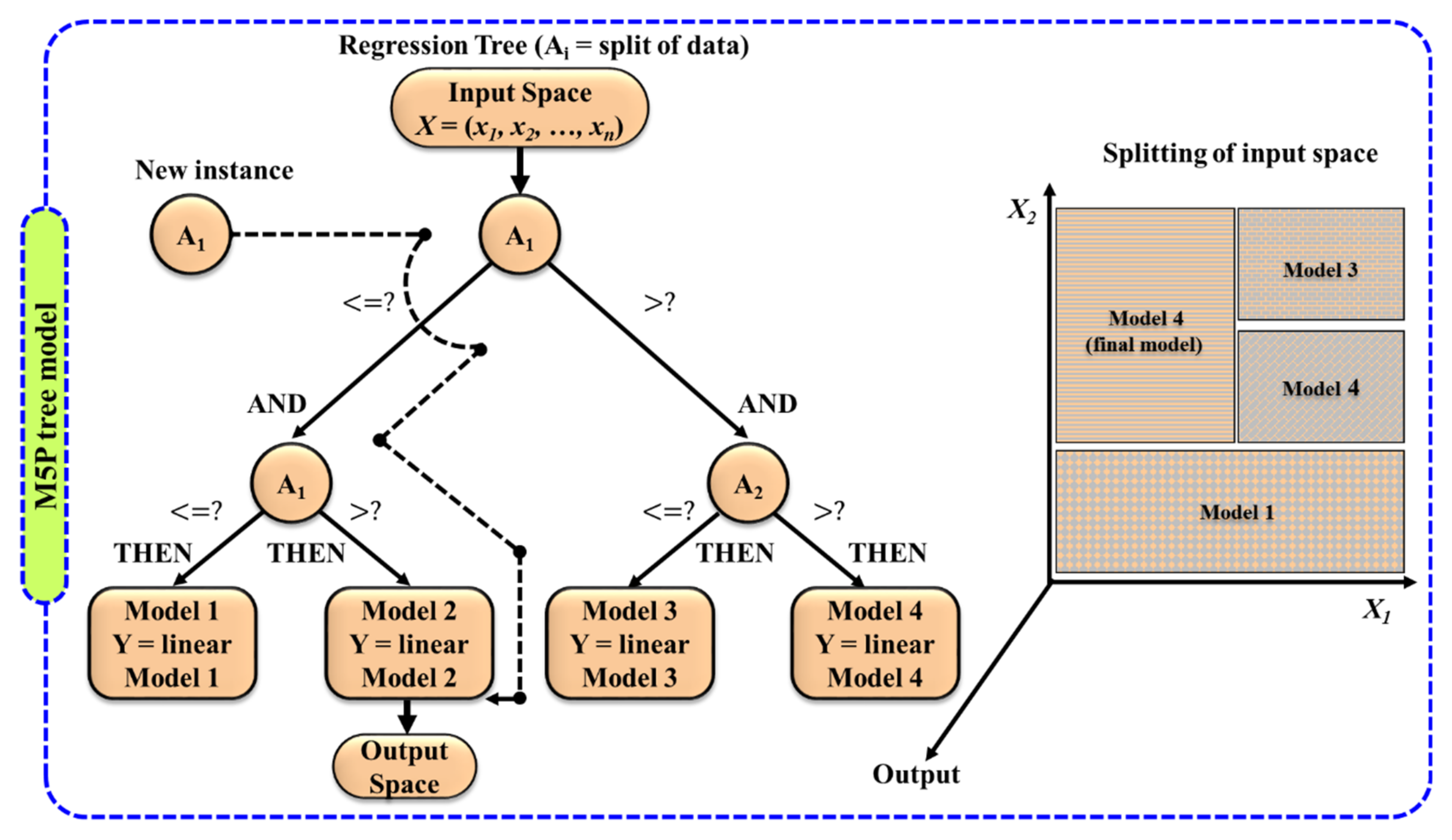
The M5P tree is a data-mining technique, projected by Quinlan [48]. The association among output (dependent)-input (independent) variables is established based on a binary decision tree having a linear regression function at the leaf (terminal nodes). The divide-and-conquer approach is applied to produce the tree-based models [49]. Figure 3 displays the well-organized topology of the M5P tree model. The construction of a decision tree involves two stages: step-1: splitting the data into subgroups to create the decision tree by utilizing the principle of the standard deviation (std) and reducing the model training error at node [50], and step-2: pruning of the overfitted tree (sample) and swapping the subtrees with linear regression functions [49]. Finally, the SDR (standard deviation reduction) is computed as [49,50]:
S D R = s t d M M j M s t d M j
where M defines a group of samples that grasps the nodes and M i signifies the subgroup of samples that have the jth consequence of the latent set. In recent times, researchers have explored the successful application of the M5P model in the simulation of several hydrological processes like drought forecasting [50], infiltration simulation [51], river discharge forecasting [52,53], reference evapotranspiration estimation [49,54], stage-discharge forecasting [55], and groundwater level prediction [56]. For comprehensive information about the M5P tree, readers refer to Quinlan [48].

2.6. Random Forest

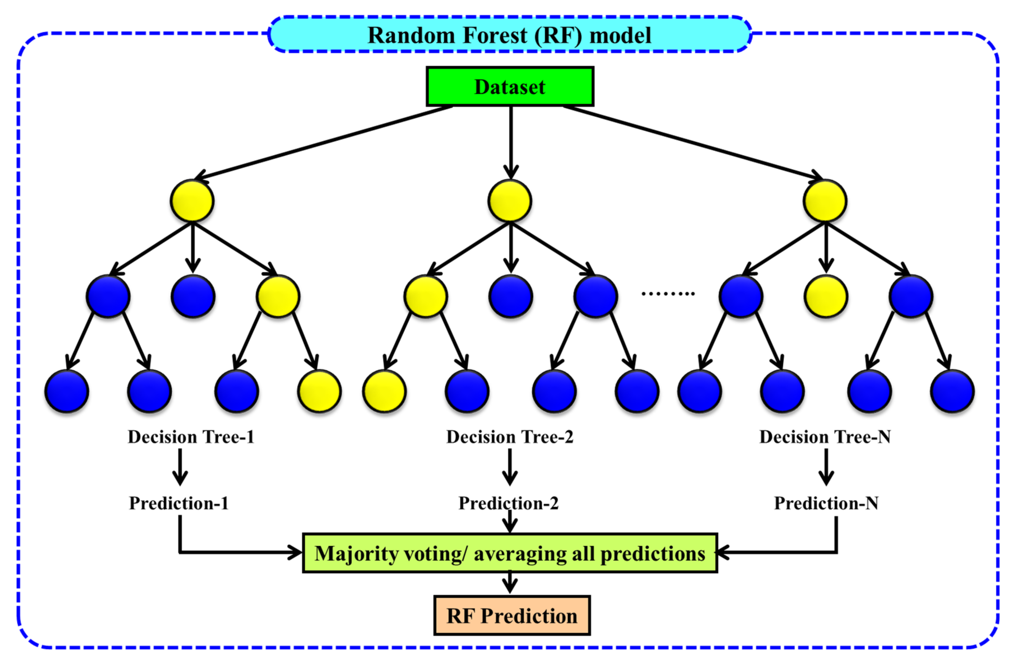
The random forest (RF) algorithm was designed by Breiman [57] for solving high-dimension classification and regression problems. Recently, the RF model received popularity in diverse fields of sciences such as, for instance, infiltration rate prediction [51], land use/land cover classification [58], and soil temperature estimation [59]. Figure 4 illustrates the hierarchical network of the RF classifier. The construction of the RF model comprises two steps: (i) an ensemble of decision trees (or classifiers) used to build the “RF” through supervised learning, and (ii) making predictions of each decision tree formed in the first step. The RF algorithm is comparatively insensitive to features of the training set and can achieve high prediction accuracy [57]. In the present study, the RF model was built by using a trial-and-error process in WEKA 3.9 software for the prediction of monthly ETo at both study locations.

2.7. Model Formulation and Statistical Indicators

Different combinations of four climatic variables, namely T, RH, u, and Rs, were used for the estimation of monthly ETo at two locations in the present research. Three combinations of four inputs were formulated based on Valiantzas’ [31,32] concept and presented in Table 3. All inputs are used for C-1, three inputs for C-2, and two inputs for C-3. All three input combinations were used to train and test the ML models.
Afterward, five statistical indicators, i.e., MAE (mean absolute error), RMSE (root-mean-square error), EC (efficiency coefficient), CC (correlation coefficient), and WI (Willmott index), were utilized to evaluate the predictive efficacy of the empirical (i.e., V-1 to V-3) and ML (i.e., SVM, M5P, RF) models used in the present study. Also, the graphical inspection includes temporal variation graphs, scatter plots, and Taylor diagrams that were used to make a clear interpretation of results yielded by the empirical and ML models. Table 4 shows the formulas of MAE, RMSE, EC, CC, and WI along with their range.

3. Results and Discussion

3.1. Model Evaluation Based on Statistical Indicators

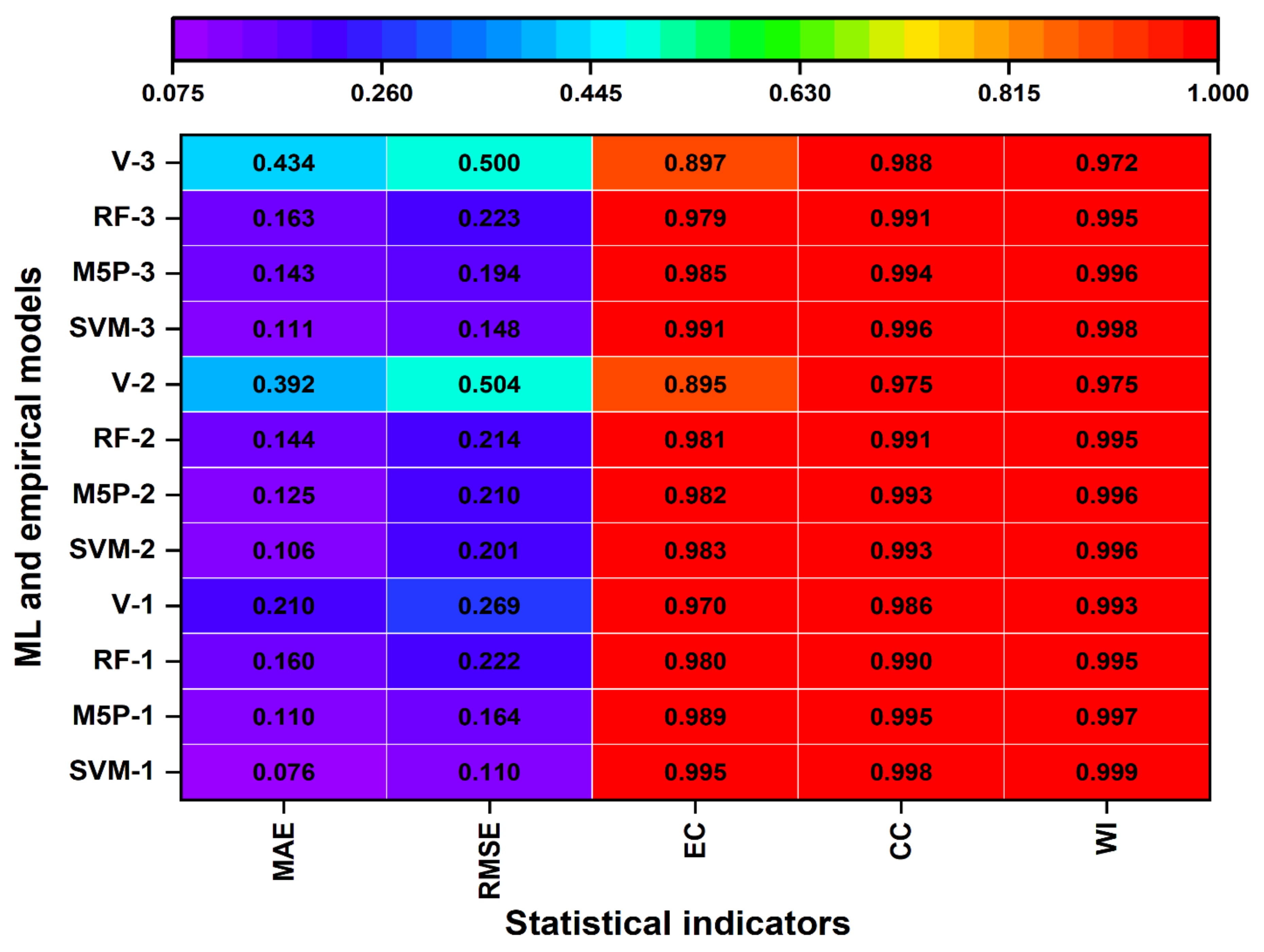
The potential of the ML models, i.e., SVM, M5P, and RF, was investigated against the empirical models (i.e., V-1, V-2, and V-3) at the Nagina and Pantnagar stations based on statistical indicators. These models were trained with 60% data (2009–2013) and tested with 40% data (2014–2016) for both locations. The values of the statistical indicators (i.e., MAE, RMSE, EC, CC, and WI) of the empirical and ML models during the validation phase on the Nagina and Pantnagar stations are presented through a heatmap (see Figure 5 and Figure 6), respectively. For Nagina, from Figure 5 for input combination C-1 corresponding to SVM-1, M5P-1, RF-1, and V-1 models, the values of MAE ranges from 0.076 to 0.210 mm/month, RMSE from 0.110 to 0.269 mm/month, EC from 0.995 to 0.970, CC from 0.998 to 0.986, and WI from 0.999 to 0.993 during the validation phase. For C-2 combination equivalent to SVM-2, M5P-2, RF-2, and V-2 models the MAE = 0.106 to 0.392 mm/month, RMSE = 0.201 to 0.504 mm/month, EC = 0.983 to 0.895, CC = 0.993 to 0.975, and WI = 0.996 to 0.975, and for C-3 combination matching to SVM-3, M5P-3, RF-3, and V-3 models the MAE = 0.111 to 0.434 mm/month, RMSE = 0.148 to 0.500 mm/month, EC = 0.991 to 0.897, CC = 0.996 to 0.988, and WI = 0.998 to 0.972 in the validation phase. It was noted from Figure 5 that the performance of kernel-based models, i.e., SVM-1, SVM-2, and SVM-3, was found to be more optimal than other models. Overall, on Nagina, the best estimation was achieved by the SVM-1 model followed by the M5P-1 model. In addition, the performance of the empirical models, i.e., V-1, V-2, and V-3, was found to be poor in comparison to the ML models at the Nagina site. The ranking of the models from best to worst is assigned as SVM-1, 2, 3 > M5P-1, 2, 3 > RF-1, 2, 3 > V-1, 2, 3, which are equivalent to C-1, 2, and 3 input combinations.
Similarly, Figure 6 illustrates the statistical indicators of the SVM, M5P, RF, and Valiantzas models in monthly ETo estimation on Pantnagar during the validation period. Here also the SVM-1, SVM-2, and SVM-3 had the lowest values of MAE (0.047, 0.141, 0.168 mm/month) and RMSE (0.063, 0.180, 0.226 mm/month), and the highest values of EC (0.999, 0.988, 0.981), CC (0.999, 0.995, 0.991), and WI (1.000, 0.997, 0.995), followed by the M5P, RF, and Valiantzas models corresponding to input combinations C-1, C-2, and C-3. The SVM model corresponding to C-1 produces better estimates than other models. In addition, the worst estimates were produced by the Valiantzas models. The models ranked from best to worst as SVM-1 > M5P-1 > V-1 > RF-1 for C-1 (i.e., T, RH, u, Rs); SVM-2 > M5P-2 > RF-2 > V-2 for C-2 (i.e., T, RH, Rs), and SVM-3 > M5P-3 > RF-3 > V-3 for C-3 (i.e., T, Rs). From this analysis, it is renowned that the SVM model with C-1 input combination including T, RH, u, and Rs climatic variables performed in a superior manner at both study stations.

3.2. Performance Evaluation Using Graphical Inspection

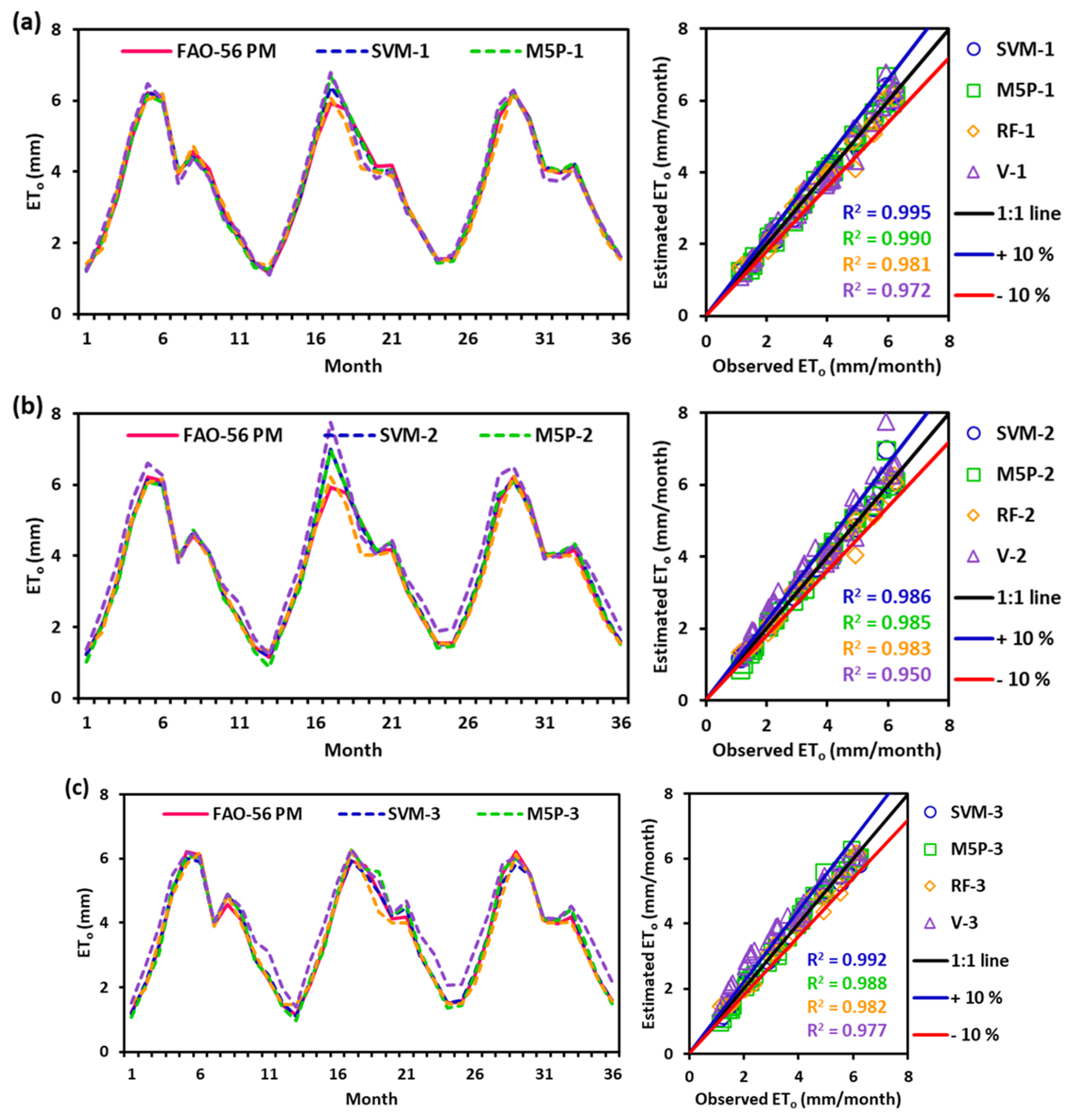
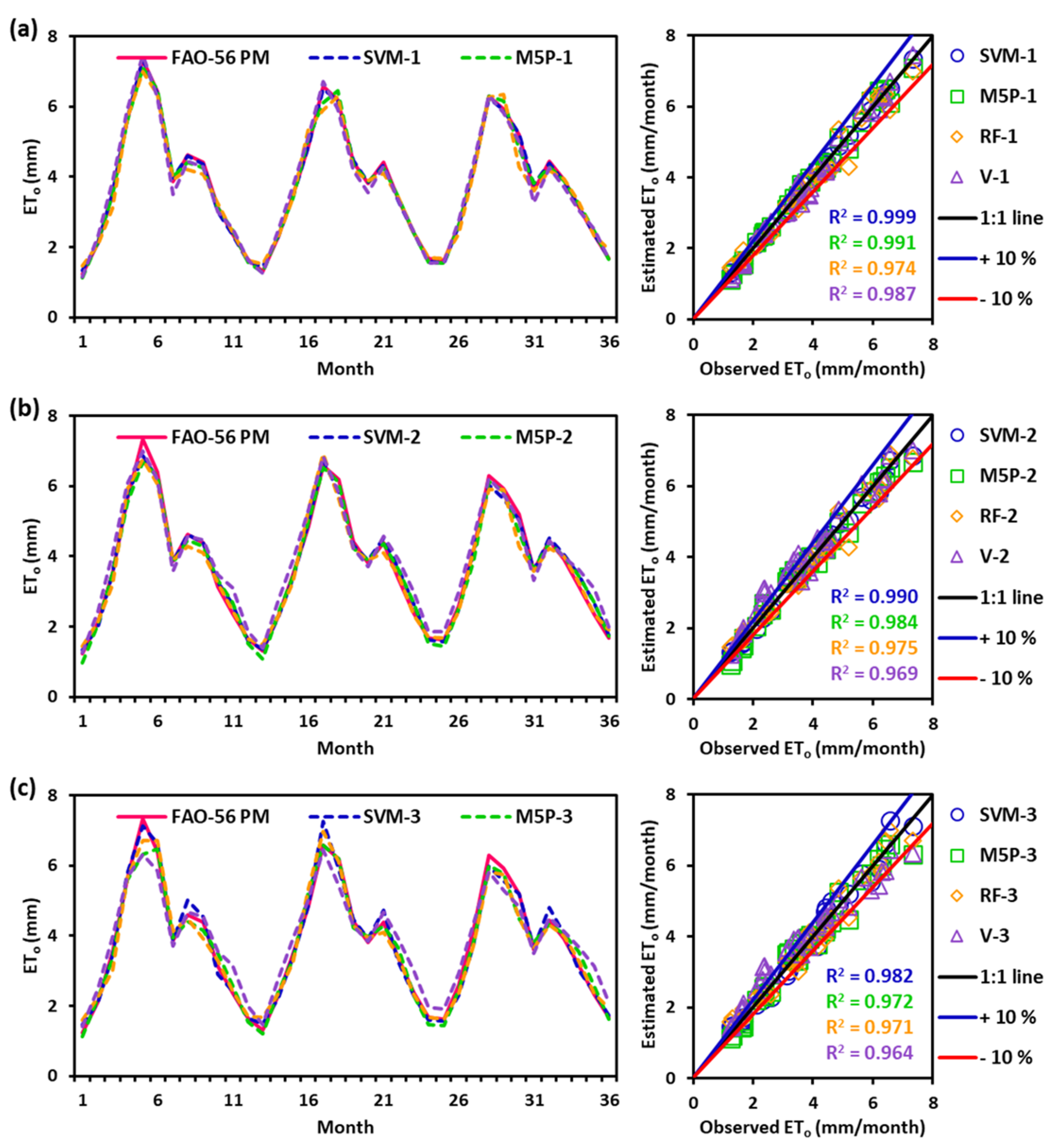
The graphical inspection was another goodness-of-fit criterion for evaluating the relative performance of the ML and empirical models during the validation phases at both stations. Figure 7a–c and Figure 8a–c illustrates the temporal variation and scatter plots of observed versus estimated monthly ETo values by the SVM, M5P, RF, and Valiantzas models equivalent to C-1, C-2, and C-3 input combinations at the Nagina and Pantnagar sites, respectively, during the validation phase. In these figures, the outputs of the four models were fitted with a 1:1 line (best-fit line) with relative error bands of ±10%, and the coefficient of determination (R2) between the observed and model outputs was also presented on the plots. If the data are concentrated or close to the 1:1 line (black line) within ±10% relative error bands, this indicates better performance of a model. These figures clearly show the higher performance of the SVM model compared to other models during the validation phase on both stations. In addition, the R2 value was found highest in the SVM-1 model (0.995) for Nagina (Figure 7a), and 0.999 for Pantnagar (Figure 8a) in the validation stage, compared to other ML and empirical models. Overall, the SVM model can be considered optimal in estimating monthly ETo in terms of the results presented in Figure 7a–c and Figure 8a–c.
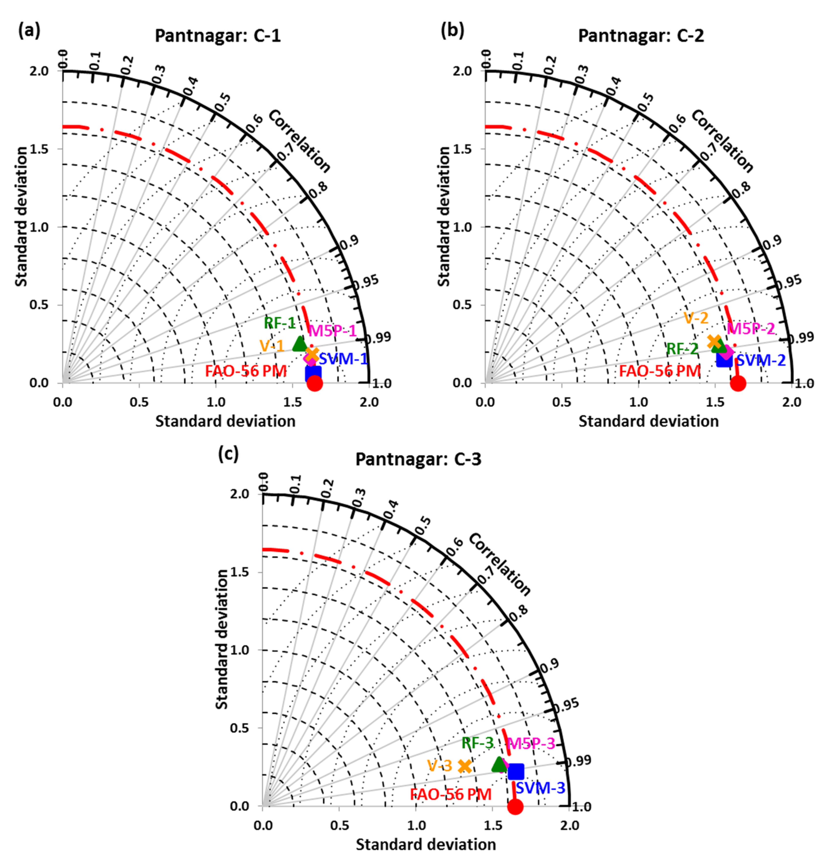
The performance of the ML and empirical models was also evaluated using the Taylor diagram [66]. The obtained result during the validation period is presented in Figure 9a–c and Figure 10a–c for Nagina and Pantnagar, respectively. The red circle on the x-axis of the Taylor diagram represents the observed monthly ETo. A model is considered better if it is near the observed point. Taylor’s diagram compares three statistics (i.e., RMSE, Std, and CC) together in a graphical way and, therefore, provides a reliable assessment of the relative performance of different models. The Taylor diagram of the models during validation showed a much better performance of SVM compared to other models at the Nagina (Figure 9a–c) and Pantnagar (Figure 10a–c) stations. In addition, the SVM-predicted monthly ETo was found better-correlated with the observed monthly ETo with less RMSE compared to other models on both stations during the validation phase. Likewise, the Std of SVM-predicted ETo was found much closer to observed ETo in comparison to other models on both stations during the validation. Therefore, SVM can be ranked as the best model in terms of the results presented in the Taylor diagram followed by the M5P, RF, and Valiantzas models at both study sites.

3.3. Discussion

Evapotranspiration is a complex hydrological process that depends on the integrated effect of several climatic variables [69]. It also governs the soil moisture, surface runoff, plant growth, and groundwater recharge for optimizing the available water resources [70]. Furthermore, it determines the processes responsible for land–atmosphere interaction or formation of the geographical environment, and weather and climate change through ground heat and moisture balance, and water balance and surface heat balance studies [70,71,72]. Similarly, Seong et al. [73] projected the implications of different potential evapotranspiration (PET) methods on streamflow under climate change in the Susquehanna River basin of the northeastern United States. They found that the streamflow projections are sensitive to the selection of the PET methods. So, the formulation of a reliable and robust model of ETo estimation is necessary for maintaining water resources and agricultural operations on farmland under a changing climate. The ML models can handle this issue very well. In this study, three ML models such as SVM, M5P, and RF were developed for monthly ETo estimation on two sites (Nagina and Pantnagar) and their outcomes were compared with empirical models. The appraisal of results shows the better feasibility of the SVM over other models at both sites. Similarly, Kaya et al. [74] estimated daily ETo in the Kosice City area of Slovakia by employing three ML models, i.e., MLP (multilayer perceptron), SVR (support vector regression), and MLR (multi-linear regression). The daily data of wind speed, relative humidity, air temperature, and solar radiation were supplied as input to these models. The performance of the ML models was evaluated against the empirical models (Hargreaves–Samani, Ritchie, & Turc), and it was found that the ML-based models provide better results than the empirical models. Kisi et al. [75] hybridized the M5 model tree with a radial basis function (RM5Tree) for estimating daily ETo at three stations (Antalya, Adana, and Isparta) in Turkey using the daily record of wind speed, relative humidity, air temperature, and solar radiation. The estimates of the RM5Tree model were compared with M5Tree, MLP, RSM (response surface method), and RBFNN (radial basis function neural network). Overall, they found the RM5Tree model provides more optimal results than the other models.
Furthermore, the findings of this research were equated to other studies conducted on ETo estimation by exploiting the ML techniques, for instance [1,9,22,76,77]. Tikhamarine et al. [11] optimized the SVR model with the WOA, MVO (multi-verse optimizer), and ALO (ant-lion optimizer) algorithms to predict the monthly ETo at the Algiers and Tlemcen weather stations located in north Algeria. They found better performance of the SVR-WOA model with WI = 0.9987, 0.9997, CC = 0.9975, 0.9995, EC = 0.9949, 0.9989, RMSE = 0.0808, 0.0617 mm/month, and MAE = 0.0658, 0.0489 for the Algiers and Tlemcen sites, respectively. Gonzalez del Cerro et al. [78] compared the predictive performance of the ANFIS against the radiation and temperature-based empirical models for estimating the daily ETo in Tamil Nadu and the Coimbatore provinces of India. Results reveal that the ANFIS-based model (MAE = 0.0008 mm/day, WI = 0.9999, and CC = 0.9999) with all climatic data, i.e., mean air temperature, relative humidity, wind speed, and solar radiation produce better estimates than the empirical models. Ahmadi et al. [79] estimated monthly ETo on six stations located in Iran by exploiting three ML models, namely the SVR, GEP (gene expression programming), SVR-IWD (intelligent water drops) against the Priestley–Taylor, and H-S Hargreaves–Samani models. A comparison of results shows that the SVR-IWD model outperformed the other models at all stations.
To this end, the aforementioned studies also recommend the effectiveness of machine learning models over the empirical models in predicting monthly ETo at both study locations.

4. Conclusions

The effectiveness of three machine learning models, such as the support vector machine (SVM), M5P tree (M5P), and random forest (RF), was investigated in predicting monthly ETo on the Nagina and Pantnagar stations from 2009 to 2016 in the present study. From the available 8-year climatic data (2009–2016) at both stations, a total of three combinations of different inputs were established to calibrate (train) and validate (test) the ML models over the empirical models (i.e., Valiantzas-1, Valiantzas-2, Valiantzas-3) based on statistical indicators and graphical inspection. The results of the evaluation demonstrate that the SVM models with the full set of climatic data, i.e., T, RH, u, and Rs, performed superior to the M5P, RF, and Valiantzas models during the validation period at both locations under this study. In addition, the predictive accuracy of the SVM-1 to SVM-3 models with respect to RMSE improved 32.9% to 59.1%, 4.3% to 60.1%, and 23.7% to 70.4%, for M5P-1 to M5P-3, RF-1 RF-3, and V-1 to V-3, respectively, on Nagina and 59.9% to 66.1%, 16.7% to 48.9%, and 19.6% to 47.6% for M5P-1 to M5P-3, RF-1 RF-3, and V-1 to V-3, respectively, on Pantnagar. This percentage analysis also reveals the supremacy of the SVM model in predicting monthly ETo at both sites under consideration. Furthermore, the performance of the empirical models was recorded as poor at both sites in comparison to the ML models. Overall, the findings of this research show that the ML models (i.e., SVM) had better efficacy and will support the irrigation engineers, agriculturists, and hydrologists to formulate smart intelligence systems for optimal planning and management of water resources at study sites.
Future research will evaluate ensemble machine learning models with different ratios of training and testing datasets obtained from multi-locations of other climatic regions. In addition, the geospatial techniques will be considered for mapping the impact of reference evapotranspiration on a spatial scale.

Author Contributions

Conceptualization, P.R. and A.M.; methodology, P.R. and A.M.; software, P.R. and A.M.; validation, P.R., P.K., N.A.-A. and A.M.; formal analysis, P.R. and A.M.; investigation, P.R., P.K., N.A.-A. and A.M.; writing—original draft preparation, P.R., P.K., N.A.-A. and A.M.; writing—review and editing, P.R., P.K., N.A.-A. and A.M.; visualization, P.R., P.K., N.A.-A. and A.M.; supervision, P.K., N.A.-A. and A.M.; project administration, N.A.-A.; funding acquisition, N.A.-A. All authors have read and agreed to the published version of the manuscript.

Funding

This research received no external funding.

Conflicts of Interest

The authors declare no conflict of interest.

References

  1. Alizamir, M.; Kisi, O.; Muhammad Adnan, R.; Kuriqi, A. Modelling Reference Evapotranspiration by Combining Neuro-Fuzzy and Evolutionary Strategies. Acta Geophys. 2020, 68, 1113–1126. [Google Scholar] [CrossRef]
  2. Awal, R.; Habibi, H.; Fares, A.; Deb, S. Estimating Reference Crop Evapotranspiration under Limited Climate Data in West Texas. J. Hydrol. Reg. Stud. 2020, 28, 100677. [Google Scholar] [CrossRef]
  3. Adamala, S.; Raghuwanshi, N.S.; Mishra, A.; Singh, R. Generalized Wavelet Neural Networks for Evapotranspiration Modeling in India. ISH J. Hydraul. Eng. 2019, 25, 119–131. [Google Scholar] [CrossRef]
  4. Pereira, L.S.; Allen, R.G.; Smith, M.; Raes, D. Crop Evapotranspiration Estimation with FAO56: Past and Future. Agric. Water Manag. 2015, 147, 4–20. [Google Scholar] [CrossRef]
  5. Feng, Y.; Cui, N.; Zhao, L.; Hu, X.; Gong, D. Comparison of ELM, GANN, WNN and Empirical Models for Estimating Reference Evapotranspiration in Humid Region of Southwest China Comparison of ELM, GANN, WNN and Empirical Models for Estimating Reference Evapotranspiration in Humid Region of Southwest. J. Hydrol. 2016, 536, 376–383. [Google Scholar] [CrossRef]
  6. Allen, R.G.; Pereira, L.S.; Raes, D.; Smith, M. Crop Evapotranspiration: Guidelines for Computing Crop Requirements. FAO Irrig. Drain. Pap. 56 1998, 300, D05109. [Google Scholar]
  7. Abdullah, S.S.; Malek, M.A.; Abdullah, N.S.; Kisi, O.; Yap, K.S. Extreme Learning Machines: A New Approach for Prediction of Reference Evapotranspiration. J. Hydrol. 2015, 527, 184–195. [Google Scholar] [CrossRef]
  8. Tabari, H.; Hosseinzadeh Talaee, P. Multilayer Perceptron for Reference Evapotranspiration Estimation in a Semiarid Region. Neural Comput. Appl. 2013, 23, 341–348. [Google Scholar] [CrossRef]
  9. Tikhamarine, Y.; Malik, A.; Kumar, A.; Souag-Gamane, D.; Kisi, O. Estimation of Monthly Reference Evapotranspiration Using Novel Hybrid Machine Learning Approaches. Hydrol. Sci. J. 2019, 64, 1824–1842. [Google Scholar] [CrossRef]
  10. Chen, Z.; Zhu, Z.; Jiang, H.; Sun, S. Estimating Daily Reference Evapotranspiration Based on Limited Meteorological Data Using Deep Learning and Classical Machine Learning Methods. J. Hydrol. 2020, 591, 125286. [Google Scholar] [CrossRef]
  11. Tikhamarine, Y.; Malik, A.; Pandey, K.; Sammen, S.S.; Souag-Gamane, D.; Heddam, S.; Kisi, O. Monthly Evapotranspiration Estimation Using Optimal Climatic Parameters: Efficacy of Hybrid Support Vector Regression Integrated with Whale Optimization Algorithm. Environ. Monit. Assess. 2020, 192, 696. [Google Scholar] [CrossRef] [PubMed]
  12. Ferreira, L.B.; da Cunha, F.F. New Approach to Estimate Daily Reference Evapotranspiration Based on Hourly Temperature and Relative Humidity Using Machine Learning and Deep Learning. Agric. Water Manag. 2020, 234, 106113. [Google Scholar] [CrossRef]
  13. Saggi, M.K.; Jain, S. Reference Evapotranspiration Estimation and Modeling of the Punjab Northern India Using Deep Learning. Comput. Electron. Agric. 2019, 156, 387–398. [Google Scholar] [CrossRef]
  14. Khosravi, K.; Daggupati, P.; Alami, M.T.; Awadh, S.M.; Ghareb, M.I.; Panahi, M.; Pham, B.T.; Rezaie, F.; Qi, C.; Yaseen, Z.M. Meteorological Data Mining and Hybrid Data-Intelligence Models for Reference Evaporation Simulation: A Case Study in Iraq. Comput. Electron. Agric. 2019, 167, 105041. [Google Scholar] [CrossRef]
  15. Wu, L.; Fan, J. Comparison of Neuron-Based, Kernel-Based, Tree-Based and Curve-Based Machine Learning Models for Predicting Daily Reference Evapotranspiration. PLoS ONE 2019, 14, e0217520. [Google Scholar] [CrossRef] [Green Version]
  16. Fan, J.; Yue, W.; Wu, L.; Zhang, F.; Cai, H.; Wang, X.; Lu, X.; Xiang, Y. Evaluation of SVM, ELM and Four Tree-Based Ensemble Models for Predicting Daily Reference Evapotranspiration Using Limited Meteorological Data in Different Climates of China. Agric. For. Meteorol. 2018, 263, 225–241. [Google Scholar] [CrossRef]
  17. Ferreira, L.B.; da Cunha, F.F.; de Oliveira, R.A.; Fernandes Filho, E.I. Estimation of Reference Evapotranspiration in Brazil with Limited Meteorological Data Using ANN and SVM—A New Approach. J. Hydrol. 2019, 572, 556–570. [Google Scholar] [CrossRef]
  18. Mehdizadeh, S.; Behmanesh, J.; Khalili, K. Using MARS, SVM, GEP and Empirical Equations for Estimation of Monthly Mean Reference Evapotranspiration. Comput. Electron. Agric. 2017, 139, 103–114. [Google Scholar] [CrossRef]
  19. Wang, S.; Lian, J.; Peng, Y.; Hu, B.; Chen, H. Generalized Reference Evapotranspiration Models with Limited Climatic Data Based on Random Forest and Gene Expression Programming in Guangxi, China. Agric. Water Manag. 2019, 221, 220–230. [Google Scholar] [CrossRef]
  20. Sarker, S.; Veremyev, A.; Boginski, V.; Singh, A. Critical Nodes in River Networks. Sci. Rep. 2019, 9, 11178. [Google Scholar] [CrossRef] [Green Version]
  21. Sarker, S. Investigating Topologic and Geometric Properties of Synthetic and Natural River Networks under Changing Climate. Dr. Diss. Univ. Cent. Fla. US 2021, 2020, 965. [Google Scholar]
  22. Ashrafzadeh, A.; Kişi, O.; Aghelpour, P.; Biazar, S.M.; Masouleh, M.A. Comparative Study of Time Series Models, Support Vector Machines, and GMDH in Forecasting Long-Term Evapotranspiration Rates in Northern Iran. J. Irrig. Drain. Eng. 2020, 146, 04020010. [Google Scholar] [CrossRef]
  23. Mehdizadeh, S.; Mohammadi, B.; Pham, Q.B.; Duan, Z. Development of Boosted Machine Learning Models for Estimating Daily Reference Evapotranspiration and Comparison with Empirical Approaches. Water 2021, 13, 3489. [Google Scholar] [CrossRef]
  24. Adnan, R.M.; Mostafa, R.R.; Islam, A.R.M.T.; Kisi, O.; Kuriqi, A.; Heddam, S. Estimating Reference Evapotranspiration Using Hybrid Adaptive Fuzzy Inferencing Coupled with Heuristic Algorithms. Comput. Electron. Agric. 2021, 191, 106541. [Google Scholar] [CrossRef]
  25. Mohammadi, B.; Mehdizadeh, S. Modeling Daily Reference Evapotranspiration via a Novel Approach Based on Support Vector Regression Coupled with Whale Optimization Algorithm. Agric. Water Manag. 2020, 237, 106145. [Google Scholar] [CrossRef]
  26. Maroufpoor, S.; Bozorg-Haddad, O.; Maroufpoor, E. Reference Evapotranspiration Estimating Based on Optimal Input Combination and Hybrid Artificial Intelligent Model: Hybridization of Artificial Neural Network with Grey Wolf Optimizer Algorithm. J. Hydrol. 2020, 588, 125060. [Google Scholar] [CrossRef]
  27. Rezaabad, M.Z.; Ghazanfari, S.; Salajegheh, M. ANFIS Modeling with ICA, BBO, TLBO, and IWO Optimization Algorithms and Sensitivity Analysis for Predicting Daily Reference Evapotranspiration. J. Hydrol. Eng. 2020, 25, 04020038. [Google Scholar] [CrossRef]
  28. Chia, M.Y.; Huang, Y.F.; Koo, C.H. Swarm-Based Optimization as Stochastic Training Strategy for Estimation of Reference Evapotranspiration Using Extreme Learning Machine. Agric. Water Manag. 2021, 243, 106447. [Google Scholar] [CrossRef]
  29. Panahi, M.; Sadhasivam, N.; Pourghasemi, H.R.; Rezaie, F.; Lee, S. Spatial Prediction of Groundwater Potential Mapping Based on Convolutional Neural Network (CNN) and Support Vector Regression (SVR). J. Hydrol. 2020, 588, 125033. [Google Scholar] [CrossRef]
  30. Borji, M.; Malekian, A.; Salajegheh, A.; Ghadimi, M. Multi-Time-Scale Analysis of Hydrological Drought Forecasting Using Support Vector Regression (SVR) and Artificial Neural Networks (ANN). Arab. J. Geosci. 2016, 9, 725. [Google Scholar] [CrossRef]
  31. Valiantzas, J.D. Simple ET0 Forms of Penman’s Equation without Wind and/or Humidity Data. I: Theoretical Development. J. Irrig. Drain. Eng. 2013, 139, 1–8. [Google Scholar] [CrossRef]
  32. Valiantzas, J.D. Simple ET0 Forms of Penman’s Equation without Wind and/or Humidity Data. II: Comparisons with Reduced Set-FAO and Other Methodologies. J. Irrig. Drain. Eng. 2013, 139, 9–19. [Google Scholar] [CrossRef] [Green Version]
  33. Afradi, A.; Ebrahimabadi, A. Comparison of Artificial Neural Networks (ANN), Support Vector Machine (SVM) and Gene Expression Programming (GEP) Approaches for Predicting TBM Penetration Rate. SN Appl. Sci. 2020, 2, 2004. [Google Scholar] [CrossRef]
  34. Biazar, S.M.; Rahmani, V.; Isazadeh, M.; Kisi, O.; Dinpashoh, Y. New Input Selection Procedure for Machine Learning Methods in Estimating Daily Global Solar Radiation. Arab. J. Geosci. 2020, 13, 431. [Google Scholar] [CrossRef]
  35. Hadi, S.J.; Tombul, M. Forecasting Daily Streamflow for Basins with Different Physical Characteristics through Data-Driven Methods. Water Resour. Manag. 2018, 32, 3405–3422. [Google Scholar] [CrossRef]
  36. Hong, H.; Pradhan, B.; Jebur, M.N.; Bui, D.T.; Xu, C.; Akgun, A. Spatial Prediction of Landslide Hazard at the Luxi Area (China) Using Support Vector Machines. Environ. Earth Sci. 2016, 75, 40. [Google Scholar] [CrossRef]
  37. Hong, H.; Pradhan, B.; Bui, D.T.; Xu, C.; Youssef, A.M.; Chen, W. Comparison of Four Kernel Functions Used in Support Vector Machines for Landslide Susceptibility Mapping: A Case Study at Suichuan Area (China). Geomat. Nat. Hazards Risk 2017, 8, 544–569. [Google Scholar] [CrossRef]
  38. Naghibi, S.A.; Pourghasemi, H.R.; Dixon, B. GIS-Based Groundwater Potential Mapping Using Boosted Regression Tree, Classification and Regression Tree, and Random Forest Machine Learning Models in Iran. Environ. Monit. Assess. 2016, 188, 44. [Google Scholar] [CrossRef]
  39. Khaledian, M.R.; Isazadeh, M.; Biazar, S.M.; Pham, Q.B. Simulating Caspian Sea Surface Water Level by Artificial Neural Network and Support Vector Machine Models. Acta Geophys. 2020, 68, 553–563. [Google Scholar] [CrossRef]
  40. Zhang, X.; Wang, J.; Zhang, K. Short-Term Electric Load Forecasting Based on Singular Spectrum Analysis and Support Vector Machine Optimized by Cuckoo Search Algorithm. Electr. Power Syst. Res. 2017, 146, 270–285. [Google Scholar] [CrossRef]
  41. Sihag, P.; Tiwari, N.K.; Ranjan, S. Support Vector Regression-Based Modeling of Cumulative Infiltration of Sandy Soil. ISH J. Hydraul. Eng. 2018, 26, 138–152. [Google Scholar] [CrossRef]
  42. Sihag, P.; Singh, V.P.; Angelaki, A.; Kumar, V.; Sepahvand, A.; Golia, E. Modelling of Infiltration Using Artificial Intelligence Techniques in Semi-Arid Iran. Hydrol. Sci. J. 2019, 64, 1647–1658. [Google Scholar] [CrossRef]
  43. Vapnik, V.N. The Nature of Statistical Learning Theory; Springer: New York, NY, USA, 1995; p. 314. [Google Scholar]
  44. Pourghasemi, H.R.; Jirandeh, A.G.; Pradhan, B.; Xu, C.; Gokceoglu, C. Landslide Susceptibility Mapping Using Support Vector Machine and GIS at the Golestan Province, Iran. J. Earth Syst. Sci. 2013, 122, 349–369. [Google Scholar] [CrossRef] [Green Version]
  45. Su, H.; Li, X.; Yang, B.; Wen, Z. Wavelet Support Vector Machine-Based Prediction Model of Dam Deformation. Mech. Syst. Signal Process. 2018, 110, 412–427. [Google Scholar] [CrossRef]
  46. Granata, F. Evapotranspiration Evaluation Models Based on Machine Learning Algorithms—A Comparative Study. Agric. Water Manag. 2019, 217, 303–315. [Google Scholar] [CrossRef]
  47. Smola, A.J.; Schölkopf, B. A Tutorial on Support Vector Regression. Stat. Comput. 2004, 14, 199–222. [Google Scholar] [CrossRef] [Green Version]
  48. Quinlan, J.R. Learning with Continuous Classes. In Proceedings of the 5th Australian Joint Conference on Artificial Intelligence, Hobart, Australia, 16–18 November 1992; Volume 92, pp. 343–348. [Google Scholar]
  49. Pal, M.; Deswal, S. M5 Model Tree Based Modelling of Reference Evapotranspiration. Hydrol. Process. 2009, 23, 1437–1443. [Google Scholar] [CrossRef]
  50. Ali, M.; Deo, R.C.; Downs, N.J.; Maraseni, T. An Ensemble-ANFIS Based Uncertainty Assessment Model for Forecasting Multi-Scalar Standardized Precipitation Index. Atmos. Res. 2018, 207, 155–180. [Google Scholar] [CrossRef]
  51. Yaseen, Z.M.; Sihag, P.; Yusuf, B.; Al-Janabi, A.M.S. Modelling Infiltration Rates in Permeable Stormwater Channels Using Soft Computing Techniques. Irrig. Drain. 2020, 70, 117–130. [Google Scholar] [CrossRef]
  52. Kisi, O.; Khosravinia, P.; Nikpour, M.R.; Sanikhani, H. Hydrodynamics of River-Channel Confluence: Toward Modeling Separation Zone Using GEP, MARS, M5 Tree and DENFIS Techniques. Stoch. Environ. Res. Risk Assess. 2019, 33, 1089–1107. [Google Scholar] [CrossRef]
  53. Taghi Sattari, M.; Pal, M.; Apaydin, H.; Ozturk, F. M5 Model Tree Application in Daily River Flow Forecasting in Sohu Stream, Turkey. Water Resour. 2013, 40, 233–242. [Google Scholar] [CrossRef]
  54. Rahimikhoob, A. Comparison between M5 Model Tree and Neural Networks for Estimating Reference Evapotranspiration in an Arid Environment. Water Resour. Manag. 2014, 28, 657–669. [Google Scholar] [CrossRef]
  55. Bhattacharya, B.; Solomatine, D.P. Neural Networks and M5 Model Trees in Modelling Water Level–Discharge Relationship. Neurocomputing 2005, 63, 381–396. [Google Scholar] [CrossRef]
  56. Sattari, M.T.; Mirabbasi, R.; Sushab, R.S.; Abraham, J. Prediction of Groundwater Level in Ardebil Plain Using Support Vector Regression and M5 Tree Model. Groundwater 2018, 56, 636–646. [Google Scholar] [CrossRef]
  57. Breiman, L. Random Forests. Mach. Learn. 2001, 45, 5–32. [Google Scholar] [CrossRef] [Green Version]
  58. Sarker, T. Role of Climatic and Non-Climatic Factors on Land Use and Land Cover Change in the Arctic: A Comparative Analysis of Vorkuta and Salekhard. Master’s Dissertation, The George Washington University, Washington, DC, USA, 2020. Available online: https://scholarspace.library.gwu.edu/etd/6969z1516 (accessed on 5 May 2022).
  59. Sihag, P.; Esmaeilbeiki, F.; Singh, B.; Pandhiani, S.M. Model-Based Soil Temperature Estimation Using Climatic Parameters: The Case of Azerbaijan Province, Iran. Geol. Ecol. Landscapes 2020, 4, 203–215. [Google Scholar] [CrossRef] [Green Version]
  60. Legates, D.R.; McCabe, G.J. Evaluating the Use of “Goodness-of-Fit” Measures in Hydrologic and Hydroclimatic Model Validation. Water Resour. Res. 1999, 35, 233–241. [Google Scholar] [CrossRef]
  61. Malik, A.; Kumar, A.; Salih, S.Q.; Kim, S.; Kim, N.W.; Yaseen, Z.M.; Singh, V.P. Drought Index Prediction Using Advanced Fuzzy Logic Model: Regional Case Study over Kumaon in India. PLoS ONE 2020, 15, e0233280. [Google Scholar] [CrossRef]
  62. Malik, A.; Kumar, A. Meteorological Drought Prediction Using Heuristic Approaches Based on Effective Drought Index: A Case Study in Uttarakhand. Arab. J. Geosci. 2020, 13, 276. [Google Scholar] [CrossRef]
  63. Willmott, C.; Matsuura, K. Advantages of the Mean Absolute Error (MAE) over the Root Mean Square Error (RMSE) in Assessing Average Model Performance. Clim. Res. 2005, 30, 79–82. [Google Scholar] [CrossRef]
  64. Nash, J.E.; Sutcliffe, J.V. River Flow Forecasting through Conceptual Models Part I—A Discussion of Principles. J. Hydrol. 1970, 10, 282–290. [Google Scholar] [CrossRef]
  65. Moriasi, D.N.; Gitau, M.W.; Pai, N.; Daggupati, P. Hydrologic and Water Quality Models: Performance Measures and Evaluation Criteria. Trans. ASABE 2015, 58, 1763–1785. [Google Scholar] [CrossRef] [Green Version]
  66. Taylor, K.E. Summarizing Multiple Aspects of Model Performance in a Single Diagram. J. Geophys. Res. Atmos. 2001, 106, 7183–7192. [Google Scholar] [CrossRef]
  67. Willmott, C.J. On the Validation of Models. Phys. Geogr. 1981, 2, 184–194. [Google Scholar] [CrossRef]
  68. Malik, A.; Kumar, A.; Rai, P.; Kuriqi, A. Prediction of Multi-Scalar Standardized Precipitation Index by Using Artificial Intelligence and Regression Models. Climate 2021, 9, 28. [Google Scholar] [CrossRef]
  69. Ye, L.; Zahra, M.M.A.; Al-Bedyry, N.K.; Yaseen, Z.M. Daily Scale Evapotranspiration Prediction over the Coastal Region of Southwest Bangladesh: New Development of Artificial Intelligence Model. Stoch. Environ. Res. Risk Assess. 2022, 36, 451–471. [Google Scholar] [CrossRef]
  70. Gao, Z.; He, J.; Dong, K.; Li, X. Trends in Reference Evapotranspiration and Their Causative Factors in the West Liao River Basin, China. Agric. For. Meteorol. 2017, 232, 106–117. [Google Scholar] [CrossRef]
  71. Sridhar, V.; Hubbard, K.G.; Wedin, D.A. Assessment of Soil Moisture Dynamics of the Nebraska Sandhills Using Long-Term Measurements and a Hydrology Model. J. Irrig. Drain. Eng. 2006, 132, 463–473. [Google Scholar] [CrossRef] [Green Version]
  72. Sridhar, V. Tracking the Influence of Irrigation on Land Surface Fluxes and Boundary Layer Climatology. J. Contemp. Water Res. Educ. 2013, 152, 79–93. [Google Scholar] [CrossRef]
  73. Seong, C.; Sridhar, V.; Billah, M.M. Implications of Potential Evapotranspiration Methods for Streamflow Estimations under Changing Climatic Conditions. Int. J. Climatol. 2018, 38, 896–914. [Google Scholar] [CrossRef]
  74. Kaya, Y.Z.; Zelenakova, M.; Üneş, F.; Demirci, M.; Hlavata, H.; Mesaros, P. Estimation of Daily Evapotranspiration in Košice City (Slovakia) Using Several Soft Computing Techniques. Theor. Appl. Climatol. 2021, 144, 287–298. [Google Scholar] [CrossRef]
  75. Kisi, O.; Keshtegar, B.; Zounemat-Kermani, M.; Heddam, S.; Trung, N.-T. Modeling Reference Evapotranspiration Using a Novel Regression-Based Method: Radial Basis M5 Model Tree. Theor. Appl. Climatol. 2021, 145, 639–659. [Google Scholar] [CrossRef]
  76. Adnan, R.M.; Chen, Z.; Yuan, X.; Kisi, O.; El-Shafie, A.; Kuriqi, A.; Ikram, M. Reference Evapotranspiration Modeling Using New Heuristic Methods. Entropy 2020, 22, 547. [Google Scholar] [CrossRef] [PubMed]
  77. Malik, A.; Kumar, A.; Ghorbani, M.A.; Kashani, M.H.; Kisi, O.; Kim, S. The Viability of Co-Active Fuzzy Inference System Model for Monthly Reference Evapotranspiration Estimation: Case Study of Uttarakhand State. Hydrol. Res. 2019, 50, 1623–1644. [Google Scholar] [CrossRef] [Green Version]
  78. Gonzalez del Cerro, R.T.; Subathra, M.S.; Manoj Kumar, N.; Verrastro, S.; Thomas George, S. Modelling the Daily Reference Evapotranspiration in Semi-Arid Region of South India: A Case Study Comparing ANFIS and Empirical Models. Inf. Process. Agric. 2020, 8, 173–184. [Google Scholar] [CrossRef]
  79. Ahmadi, F.; Mehdizadeh, S.; Mohammadi, B.; Pham, Q.B.; DOAN, T.N.C.; Vo, N.D. Application of an Artificial Intelligence Technique Enhanced with Intelligent Water Drops for Monthly Reference Evapotranspiration Estimation. Agric. Water Manag. 2021, 244, 106622. [Google Scholar] [CrossRef]
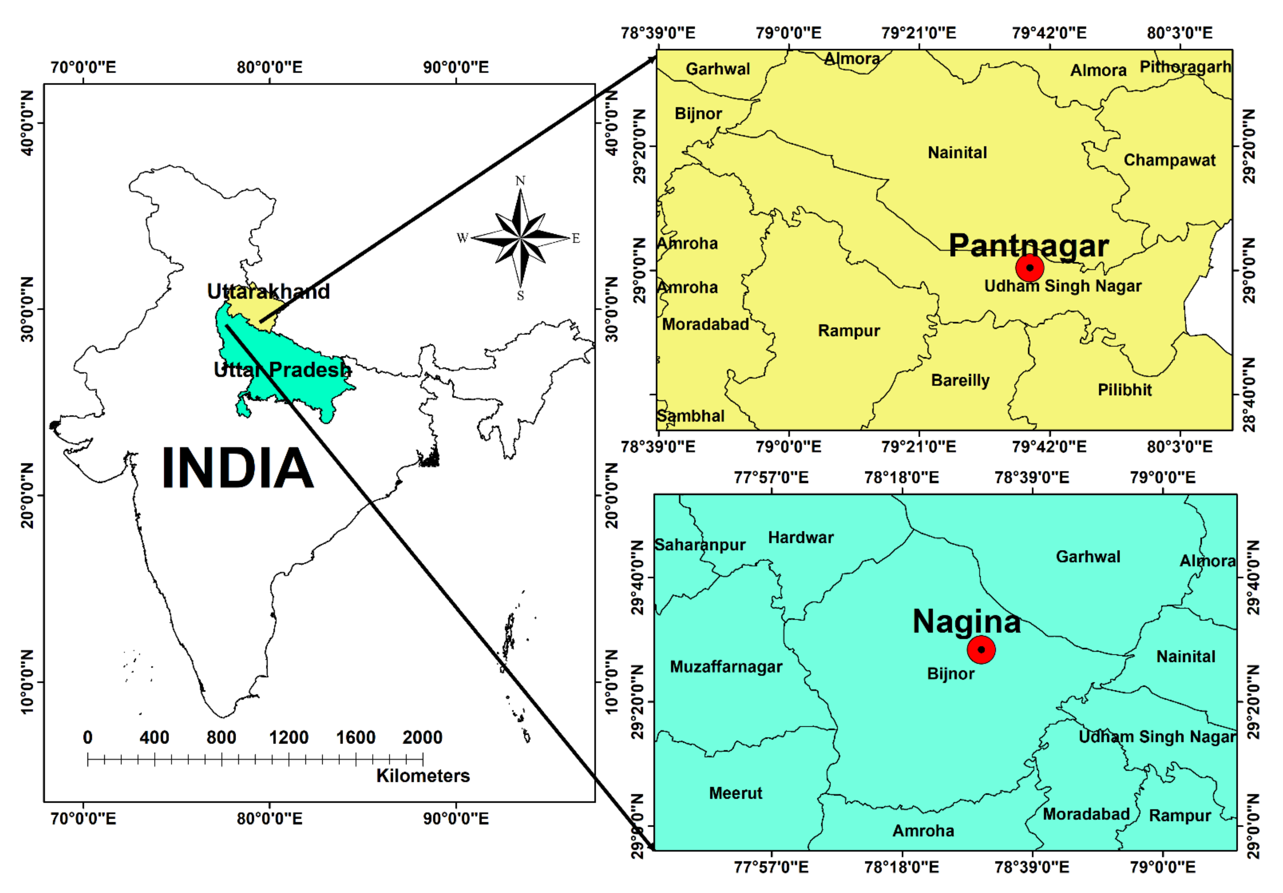
Figure 1. Location map of study sites.
Sustainability 14 05771 g001
Figure 2. The architecture of the SVM model.
Sustainability 14 05771 g002
Figure 3. Structure of the M5P model.
Sustainability 14 05771 g003
Figure 4. Typical structure of the RF model.
Sustainability 14 05771 g004
Figure 5. Heatmap of statistical indicators values produced by ML and empirical models corresponding to C-1 to C-3 input combinations in the validation phase at the Nagina station.
Sustainability 14 05771 g005
Figure 6. Heatmap of statistical indicators values produced by ML and empirical models corresponding to C-1 to C-3 input combinations in the validation phase at the Pantnagar station.
Sustainability 14 05771 g006
Figure 7. Comparison of observed (FAO-56 PM) against estimated ETo values by the ML and Valiantzas models corresponding to (a) C-1, (b) C-2, and (c) C-3 input combinations during the validation stage at Nagina station.
Sustainability 14 05771 g007
Figure 8. Comparison of observed (FAO-56 PM) against predicted ETo values by the ML and Valiantzas models corresponding to (a) C-1, (b) C-2, and (c) C-3 input combinations during the validation stage at Pantnagar station.
Sustainability 14 05771 g008
Figure 9. Taylor’s diagram of ML and empirical models corresponding to (a) C-1, (b) C-2, and (c) C-3 input combinations during the validation stage at Nagina station.
Sustainability 14 05771 g009
Figure 10. Taylor’s diagram of ML and empirical models corresponding to (a) C-1, (b) C-2, and (c) C-3 input combinations during the validation stage at Pantnagar station.
Sustainability 14 05771 g010
Table 1. Statistical and geographical information of study sites.
StationStatistical PropertiesClimatic VariablesGeographical Properties
T (°C)RH (%)u (m/s)Rs (MJ/m2/month)ETo (mm/month)Longitude (E)Latitude (N)Altitude (m)Climatic Data (Year)
NaginaMinimum10.90024.6000.2788.3001.14078°25′59″29°26′35″282.02009–2016
Maximum33.00088.0001.94625.0006.760
Mean22.99471.9651.04917.0893.572
Standard deviation6.41211.8910.4224.6111.573
Skewness−0.393−1.2350.210−0.0350.255
Kurtosis−1.2741.667−0.925−0.989−0.958
PantnagarMinimum11.45041.5000.5848.2001.24079°38′00″29°00′00″243.82009–2016
Maximum33.00086.5002.75224.7007.680
Mean23.60967.8391.41516.6343.831
Standard deviation6.20411.3030.5274.4131.692
Skewness−0.433−0.7210.375−0.0640.459
Kurtosis−1.255−0.473−0.435−0.818−0.629
Table 2. Formulas of empirical models used at study sites.
ModelEquationReference
V-1 E T o = 0.0393 R s T + 9.5 0.19 R s 0.6 φ 0.15 + 0.048 T + 20 1 R H 100 u 2 0.7 [31,32]
V-2 E T o = 0.0393 R s T + 9.5 0.19 R s 0.6 φ 0.15 + 0.078 T + 20 1 R H 100 [31,32]
V-3 E T o = 0.0393 R s T + 9.5 0.19 R s 0.6 φ 0.15 + 0.0061 T + 20 1.12 T T m i n 2 0.7 [31,32]
Note: T = mean air temperature (°C), u 2 = wind speed at 2 m height above ground (m/s), φ = latitude of site (rad), and T m i n = minimum temperature (°C).
Table 3. Different input combinations for the formulation of ML models at study sites.
CombinationInputsOutputML Models
C-1T, RH, u, RsEToSVM, M5P, RF
C-2T, RH, RsEToSVM, M5P, RF
C-3T, RsEToSVM, M5P, RF
Table 4. Formulas of different performance indicators.
EquationRangeReference
M A E = i = 1 N E T o e s t , i E T o o b s , i N (0 < MAE < ∞)[60,61]
R M S E = i = 1 N ( E T o o b s , i E T o e s t , i ) 2 N (0 < RMSE < ∞)[62,63]
E C = 1 i = 1 N ( E T o o b s , i E T o e s t , i ) 2 i = 1 N ( E T o o b s , i E T o o b s ¯ ) 2 (−∞ < EC < 1)[64,65]
C C = i = 1 N E T o o b s , i E T o o b s ¯     E T o e s t , i E T o e s t ¯   i = 1 N ( E T o o b s , i E T o o b s ¯ ) 2     i = 1 N ( E T o e s t , i E T o e s t ¯ ) 2               (−1 < CC < 1)[65,66]
W I = 1 i = 1 N ( E T o e s t , i E T o o b s , i ) 2 i = 1 N ( E T o e s t , i E T o o b s ¯ + E T o o b s , i E T o o b s ¯ ) 2 (0 < WI ≤ 1)[67,68]
Note: E T o p r e , i , and E T o o b s , i = estimated and observed monthly reference evapotranspiration values at an ith time step, N = number of observations. E T o o b s ¯ , and E T o p r e ¯ = mean of observed and predicted monthly reference evapotranspiration.
Publisher’s Note: MDPI stays neutral with regard to jurisdictional claims in published maps and institutional affiliations.