Demand Management for Resilience Enhancement of Integrated Energy Distribution System against Natural Disasters

Abstract

For energy sustainability, the integrated energy distribution system (IEDS) is an efficient and clean energy system, which is based on the coordinated operation of a power distribution network, a gas distribution network and a district heating system. In this paper, considering the damage of natural disasters to IEDS, a demand management strategy is proposed to improve resilience of IEDS and ensure stable operation, which is divided into three stages. In the first stage, the electricity, natural gas and thermal energy are co-optimized in the simulating fault state to develop the importance ranking of transmission lines and gas pipelines. In the second stage, the natural disasters are classified as surface natural disasters and geological natural disasters. According to the types of natural disasters, the demand management strategy includes semi-emergency demand management scheme and full-emergency demand management scheme in the electrical resilience mode and the integrated resilience mode, respectively. In the third stage, the non-sequential Monte-Carlo simulation and scenario reduction algorithm are applied to describe potential natural disaster scenarios. According to the importance ranking of transmission lines and gas pipelines, a demand management strategy is formulated. Finally, the proposed strategy is applied on an IEEE 33-bus power system and a 19-node natural gas system. Its effectiveness is verified by numerical case studies.

1. Introduction

With the development of society and economy, predatory energy consumption has caused environmental pollution [1] and energy crisis [2]. The integrated energy distribution system (IEDS) [3,4] takes full account of electricity, natural gas, heat and other forms of energy coupling. It can achieve the effect of energy mutual benefit according to the energy consumption characteristics of electricity, natural gas and heat. Hence, IEDS is an efficient and clean energy system.

On the other hand, frequent natural disasters have severely affected the energy system. In 2011, the Great East Japan Earthquake caused power outages in 8.71 million homes in the affected area [5]. In 2012, approximately 7.5 million customers suffered power outages in the Hurricane Sandy in New York and the disaster caused an economic loss of 65 billion US dollars [6]. Many typhoons from the Pacific will land in China every year. For example, Jiangsu Province was hit by a typhoon in 2016, which caused two 500-kV transmission lines, four 220-kV transmission lines, and eight 110-kV transmission lines to trip and left many customers without power [7]. In this regard, it is necessary and exigent to enhance the IEDS resilience. The IEDS resilience is derived from the extension of power system resilience, which can be defined as the ability to anticipate, resist, absorb and recover from disruptions caused by extreme natural disasters such as earthquakes and hurricanes [8].

At present, the previous studies mainly focused on power system resilience [9,10,11,12,13,14,15]. Two types of strategies can be adopted to enhance resilience: operational measures [9,10,11] and hardening measures [12,13,14,15]. The operational measures include scheduling flexible back-up resources [9], using decentralized control strategies [10] and altering network topology [11]. The study in [9] proposes dispatching mobile emergency generators to restore critical loads and improve power distribution system resilience. In [10], the networked micro-grids (MGs) are scheduled by a decentralized control strategy, which can improve power quality by supporting and interchanging electricity among the networked MGs. In [11], power grid reconfiguration is adopted in an active distribution system to reduce load demand response and improve power grid resilience. On the other hand, the hardening measures mean physically enhancing the infrastructure to reduce its susceptibility to disruptions [12], In [13], a tri-level defender-attacker-defender (DAD) model is proposed and its result can provide the system hardening decisions.

Due to the increasing interaction among the electricity distribution system, natural gas distribution system and district heating system, it is not suitable to consider power system resilience solely and it is necessary to consider integrated energy system resilience. However, the literature contains little research on IEDS resilience [14,15]. The study in [14] considers that the overhead power grid can be hardened by replacing fragile overhead transmission lines with underground natural gas pipelines and proposes a two-stage robust model to formulate this issue. Combined with the natural gas system, the DAD model is further expanded in [15] to accommodate electricity and gas storage facilities. The existing enhanced resilience methods in the aforementioned research are listed in

Table 1. The existing enhanced resilience methods.

System Types	References	Enhanced Resilience Methods
Power system	[9]	Scheduling flexible back-up resources
	[10]	Decentralized control strategy for MGs
	[11]	Grid reconfiguration
	[12]	Enhancing infrastructure
	[13]
Integrated energy system	[14]	Enhancing infrastructure
	[15]
	This paper	Demand management

.

Although the IEDS resilience has not been fully studied yet, there is much research focusing on the operation of integrated energy system [16,17,18,19]. In [16], an integrated framework based on the Newton-Raphson technique is proposed to solve the steady-state energy flow among electrical, natural gas, and district heating networks. Furthermore, the study in [17] proposes a coordinated optimal operation method of the regional energy internet, considering the combined cooling, heating and power (CCHP) units. The study in [18] proposes a robust day-ahead scheduling model for electricity and natural gas system, which minimizes the total cost including fuel cost, spinning reserve cost and cost of operational risk while ensuring the feasibility for all scenarios within the uncertainty set. In particular, the study in [19] proposes a novel linear method for Weymouth equation of natural gas system, which develops a more robust, flexible and tractable formulation of the integrated power and gas network.

The above research on the integrated energy system operation lay the foundation for IEDS resilience. Therefore, motivated by the aforementioned facts, this paper proposes a novel demand management strategy for improving the resilience of the power distribution network and gas distribution network in different types of natural disasters. The demand management strategy is divided into three stages. In the first stage, the critical transmission lines and gas pipelines are identified by co-optimizing electricity, natural gas and thermal energy under the assumptive fault. In other word, the importance ranking of transmission lines and gas pipelines are developed by simulating fault state. In the second stage, the natural disasters are classified as surface natural disasters (SNDs) and geological natural disasters (GNDs). The demand management strategy includes two modes. In the case of SNDs, the demand management strategy adopts the electrical resilience mode, in which the overhead transmission lines in power distribution system will be damaged, while the underground gas pipelines in gas distribution system still work without fault. In the case of GNDs, the demand management strategy adopts the integrated resilience mode, in which both overhead transmission lines and underground gas pipelines will be damaged. In the third stage, the non-sequential Monte-Carlo simulation and scenario reduction algorithm are applied to describe potential natural disaster scenarios. According to the importance ranking of transmission lines and gas pipelines, the demand management strategy is formulated. The advantages of the proposed strategy are demonstrated by numerical case studies.

The objective of the study is to propose a demand management strategy for resilience enhancement of IEDS against natural disasters and prove the effectiveness and practicality of this strategy. The major contributions of this paper are summarized as follows:

(1) Aiming at improving the IEDS resilience, this paper proposes a demand management strategy, which innovatively expands the traditional demand management in the power system.

(2) The demand management strategy includes semi-emergency demand management scheme and full-emergency demand management scheme in the electrical resilience mode and the integrated resilience mode, respectively. In the electrical resilience mode, gas distribution system can operate normally and play a role of energy storage to help power distribution system reduce demand response load. In the integrated resilience mode, the whole integrated energy system suffers damage and demand management is required.

(3) The demand management strategy is formulated in accordance with the importance of transmission lines and gas pipelines, taking into account the impact of the transmission grid and gas transmission network structure on demand management, which can increase the resilience of IEDS and reduce the economic subsidy cost of demand management.

The rest of this paper is organized as follows. The type of natural disasters, the stochastic approaches, and the framework of demand management strategy are discussed in Section 2. Then, Section 3 presents the scheduling model for the IEDS. In Section 4, numerical results are provided to validate the proposed strategy. Finally, Section 5 draws main conclusions in this paper.

2. The Demand Management Strategy for the IEDS under Natural Disasters

2.1. The Type of Natural Disasters

In this paper, natural disasters are divided into SNDs and GNDs according to whether the underground gas pipeline is destroyed or not. The SNDs include hurricane, typhoon and blizzard, while the GNDs include earthquake, landslide and mud-rock flow. The typical surface natural disaster and geological natural disaster are shown in Figure 1.

Because the overhead transmission lines are exposed to the environment, they are vulnerable to SNDs, such as typhoons and hurricanes. However, the underground gas pipelines have a certain resistibility to SNDs, so the gas distribution system can operate normally in the case of SNDs. Hence, the gas distribution system plays a role of energy storage to helps power distribution system improve resilience. In summary, the mode in which the overhead transmission lines are destroyed and the underground gas pipelines are not destroyed is called the electrical resilience mode.

On the other hand, both overhead transmission lines and underground gas pipelines may be damaged by the GNDs. In this case, the underground gas pipelines will be destroyed, and the gas distribution system also needs to be restored. Therefore, the mode in which the overhead transmission lines and the underground gas pipelines are destroyed is called the integrated resilience mode.

In this paper, the proposed demand management strategy can be applied to two types of natural disasters. The main difference between the two modes is whether the gas loads need to be reduced in the recovery process.

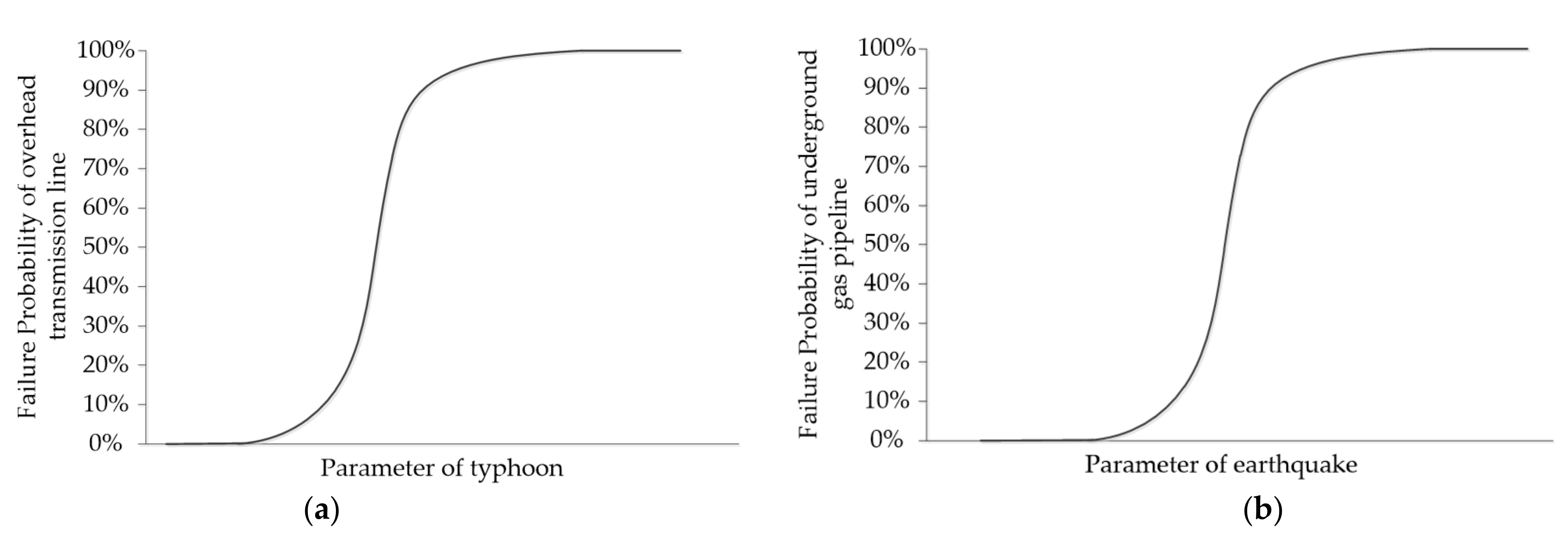
2.2. The Fragility Curves and Stochastic Approaches

The non-sequential Monte-Carlo simulation method generates many disaster scenarios with the random parameters of typhoon or earthquake. In order to get a typical disaster scenario, the scenario reduction algorithm is applied to reduce the number of samples. Then, as a calculation result of the scenario reduction algorithm, several main scenarios and their weights are derived. A detailed description of this algorithm can be found in [20].

The failure probabilities of the overhead transmission lines and underground gas pipelines in each simulated scenario are provided through their fragility curves, which express their failure probability as a function of the disaster parameter. The generic fragility curves of the overhead transmission lines and underground gas pipelines are shown in Figure 2 [8].

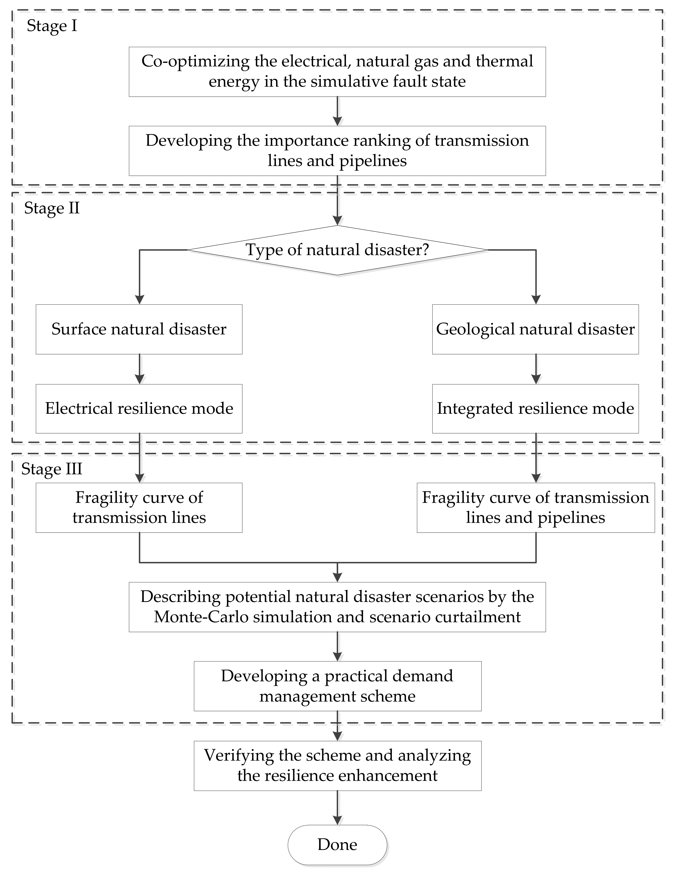
2.3. The Framework of the Demand Management Strategy

As noted earlier, the demand management strategy is divided into three stages and its framework is depicted in Figure 3.

The first stage is the pre-disaster stage, in which the power distribution system, gas distribution system and district heating system co-optimize under the assumptive fault to identify critical transmission lines and gas pipelines, which is formulated in Section 3. Then, the second stage is mainly to distinguish the modes of demand management strategy corresponding to different types of natural disasters. On this basis, the third stage generates the simulated scenarios and develops the demand management scheme.

3. Model Formulation

3.1. Objective Function

The goal of scheduling is to minimize the total operation cost of IEDS as shown in (1). Please refer to the Abbreviations for the explanation of the variables, indices, sets and parameters.

$$\begin{gathered} \min \{{\displaystyle \sum }_{s=1}^{N_s}{\lambda }_s({\displaystyle \sum }_{t=1}^T(\underset{i}{\underbrace{{\displaystyle \sum }_{i^{pe}\in {\delta }_{pe}\left(b\right)}{c}_t^p{p}_{i^{pe},t,s}^{pur}}}+\underset{\mathrm{ii}}{\underbrace{{\displaystyle \sum }_{i^{pe}\in {\delta }_{pe}\left(b\right)}{c}_t^q{q}_{i^{pe},t,s}^{pur}}}+\underset{\mathrm{iii}}{\underbrace{{\displaystyle \sum }_{i^{pg}\in {\delta }_{pg}\left(n\right)}{c}_t^f{f}_{i^{pg},t,s}^{pur}}}+\underset{\mathrm{iv}}{\underbrace{{\displaystyle \sum }_{i^{CHP}\in {\delta }_{CHP}\left(b\right)}{c}_{i^{CHP}}^q{q}_{i^{CHP},t,s}^{CHP}}} \\ +\underset{v}{\underbrace{{\displaystyle \sum }_{b=1}^{N_{bus}}{\pi }^p{p}_{b,t,s}^{demand}}}+\underset{\mathrm{vi}}{\underbrace{{\displaystyle \sum }_{b=1}^{N_{bus}}{\pi }^q{q}_{b,t,s}^{demand}}}+\underset{\mathrm{vii}}{\underbrace{{\displaystyle \sum }_{n=1}^{N_{node}}{\pi }^f{f}_{n,t,s}^{demand}}}+\underset{\mathrm{viii}}{\underbrace{{\pi }^h{h}_{t,s}^{demand}}}+\underset{\mathrm{ix}}{\underbrace{{\displaystyle \sum }_{i^w\in {\delta }_w\left(b\right)}{\kappa }_{i^w}^w{p}_{i^w,t,s}^{w,cut}}}))\} \end{gathered}$$

(1)

The goal of the optimization is to minimize operation cost. The operation cost includes 9 parts, which can be divided into 3 categories. The first category is purchasing cost, including active power purchased (i) from electricity transmission system, reactive power purchased (ii) from electricity transmission system, natural gas purchased (iii) from gas transmission system, reactive power purchased (iv) from combined heating and power (CHP) units. The second category is demand response cost, including active power load demand response (v), reactive power load demand response (vi), gas load demand response (vii), and heat load demand response (viii). The third category is penalty cost, including penalty cost of wind power curtailment (ix).

3.2. The Power Distribution System Constraints

The branch flow model is widely applied to compute the alternative current power flow of a power distribution system, but it is not suitable for optimization problems, because this model includes the power flow constraints, which is non-convex. For this difficulty, the second-order cone (SOC) relaxation is employed to relax the non-convex constraints in the branch flow model [21]. In detail, following the SOC relaxation method, the power flow equality constraints are replaced by inequality constraints and this modification still ensures the exactness, so the non-convex branch flow model is converted to the DistFlow model. Furthermore, the DistFlow model can be linearized to formulate microgrid operation constraints. In fact, the linear DistFlow model has been extensively used and justified in power distribution systems.

The linear DistFlow model gives constraints (2)–(13).

$$\begin{array}{l}{\displaystyle \sum _{i^{pe}\in {\delta }_{pe}(b)}{p}_{i^{pe},t,s}^{pur}}+{\displaystyle \sum _{\begin{array}{l}{i}^{le}\in {\delta }_{le}(b)\\ j^{ls}\in \mathcal{l}(i^{le})\end{array}}{p}_{i^{le}{j}^{ls},t,s}^l}+{\displaystyle \sum _{i^{CHP}\in {\delta }_{CHP}(b)}{p}_{i^{CHP},t,s}^{CHP}}+{\displaystyle \sum _{i^w\in {\delta }_w(b)}{p}_{i^w,t,s}^w}\\ ={\displaystyle \sum _{\begin{array}{l}{i}^{ls}\in {\delta }_{ls}(b)\\ j^{le}\in \mathcal{l}(i^{ls})\end{array}}{p}_{i^{ls}{j}^{le},t,s}^l}+{\displaystyle \sum _{i^{EHP}\in {\delta }_{EHP}(b)}{p}_{i^{EHP},t,s}^{EHP}}+p_{b,t,s}^{load}-p_{b,t,s}^{demand} \forall b,\forall t,\forall s\end{array}$$

(2)

$$\begin{array}{l}{\displaystyle \sum _{i^{pe}\in {\delta }_{pe}(b)}{q}_{i^{pe},t,s}^{pur}}+{\displaystyle \sum _{\begin{array}{l}{i}^{le}\in {\delta }_{le}(b)\\ j^{ls}\in \mathcal{l}(i^{le})\end{array}}{q}_{i^{le}{j}^{ls},t,s}^l}+{\displaystyle \sum _{i^{CHP}\in {\delta }_{CHP}(b)}{q}_{i^{CHP},t,s}^{CHP}}+{\displaystyle \sum _{i^w\in {\delta }_w(b)}{q}_{i^w,t,s}^w}\\ ={\displaystyle \sum _{\begin{array}{l}{i}^{ls}\in {\delta }_{ls}(b)\\ j^{le}\in \mathcal{l}(i^{ls})\end{array}}{q}_{i^{ls}{j}^{le},t,s}^l}+q_{b,t,s}^{load}-q_{b,t,s}^{demand} \forall b,\forall t,\forall s\end{array}$$

(3)

$$V_{i^{ls},t,s}-V_{j^{le},t,s}=\frac{p_{i^{ls}{j}^{le},t,s}^l{r}_{i^{ls}{j}^{le}}+q_{i^{ls}{j}^{le},t,s}^l{x}_{i^{ls}{j}^{le}}}{V_{base}} i^{ls}\in {\delta }_{ls}(b),j^{le}\in \mathcal{l}(i^{ls}),\forall t,\forall s$$

(4)

$$-{\overline{p}}_{i^{ls}{j}^{le}}^l\le p_{i^{ls}{j}^{le},t,s}^l\le {\overline{p}}_{i^{ls}{j}^{le}}^l i^{ls}\in {\delta }_{ls}(b),j^{le}\in \mathcal{l}(i^{ls}),\forall t,\forall s$$

(5)

$$-{\overline{q}}_{i^{ls}{j}^{le}}^l\le q_{i^{ls}{j}^{le},t,s}^l\le {\overline{q}}_{i^{ls}{j}^{le}}^l i^{ls}\in {\delta }_{ls}(b),j^{le}\in \mathcal{l}(i^{ls}),\forall t,\forall s$$

(6)

$$0\le p_{i^{pe},t,s}^{pur}\le {\overline{p}}^{pur} i^{pe}\in {\delta }_{pe}(b),\forall t,\forall s$$

(7)

$$0\le q_{i^{pe},t,s}^{pur}\le {\overline{q}}^{pur} i^{pe}\in {\delta }_{pe}(b),\forall t,\forall s$$

(8)

$${\underset{\_}{V}}_b\le V_{b,t,s}\le {\overline{V}}_b \forall b,\forall t,\forall s$$

(9)

$$0\le p_{b,t,s}^{demand}\le p_{b,t,s}^{load} \forall b,\forall t,\forall s$$

(10)

$$0\le q_{b,t,s}^{demand}\le q_{b,t,s}^{load} \forall b,\forall t,\forall s$$

(11)

$$p_{i^w,t,s}^w={\overline{p}}_{i^w,t,s}^w-p_{i^w,t,s}^{w,cut} i^w\in {\delta }_w(b),\forall t,\forall s$$

(12)

$$q_{i^w,t,s}^w=\tan (arccos({\varphi }_{i^w}))p_{i^w,t,s}^w i^w\in {\delta }_w(b),\forall t,\forall s$$

(13)

Specifically, (2) and (3) imply active power balance and reactive power balance, which means that the active (or reactive) power injection amount is equivalent to outflow amount at each bus. (4) is the DistFlow equation, which relates the active power and reactive power flows of a transmission line to the voltage magnitude of its two terminal buses. (5) and (6) denote active power limit and reactive power limit on overhead transmission lines, respectively. (7) and (8) refer to the active (or reactive) power purchasing limits. (9) gives voltage limit at each bus. (10) and (11) imply the load demand response of active power and reactive power, respectively. (12) and (13) describe power outputs of wind generators.

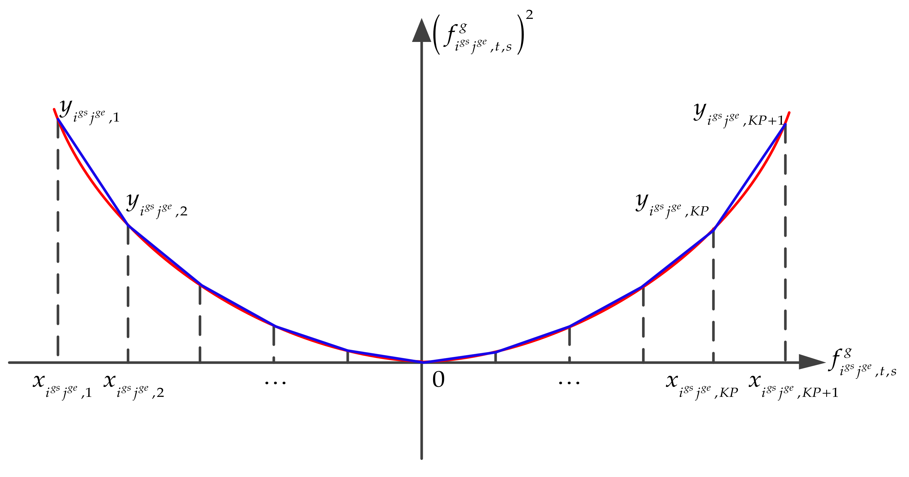
3.3. The Gas Distribution System Constraints

The operation constraints of the gas distribution system are shown in (14)–(19).

$$\begin{array}{l}{\displaystyle \sum _{i^{pg}\in {\delta }_{pg}(n)}{f}_{i^{pg},t,s}^{pur}}+{\displaystyle \sum _{\begin{array}{l}{i}^{ge}\in {\delta }_{ge}(n)\\ j^{gs}\in g(i^{ge})\end{array}}{f}_{i^{ge}{j}^{gs},t,s}^g}={\displaystyle \sum _{\begin{array}{l}{i}^{gs}\in {\delta }_{gs}(n)\\ j^{ge}\in g(i^{gs})\end{array}}{f}_{i^{gs}{j}^{ge},t,s}^g}\\ +{\displaystyle \sum _{i^{CHP}\in {\delta }_{CHP}(n)}{f}_{i^{CHP},t,s}^{CHP}}+{\displaystyle \sum _{i^{boi}\in {\delta }_{boi}(n)}{f}_{i^{boi},t,s}^{boi}}+f_{n,t,s}^{load}-f_{n,t,s}^{demand} \forall n,\forall t,\forall s\end{array}$$

(14)

$$-{\overline{f}}_{i^{gs}{j}^{ge}}^g\le f_{i^{gs}{j}^{ge},t,s}^g\le {\overline{f}}_{i^{gs}{j}^{ge}}^g i^{gs}\in {\delta }_{gs}(n),j^{ge}\in \mathcal{l}(i^{gs}),\forall t,\forall s$$

(15)

$$0\le f_{i^{pg},t,s}^{pur}\le {\overline{f}}^{pur} i^{pg}\in {\delta }_{pg}(n),\forall t,\forall s$$

(16)

$${\underset{\_}{z}}_n\le z_{n,t,s}\le {\overline{z}}_n \forall n,\forall t,\forall s$$

(17)

$$0\le f_{n,t,s}^{demand}\le f_{n,t,s}^{load} \forall n,\forall t,\forall s$$

(18)

$$f_{i^{gs}{j}^{ge},t,s}^g=K_{i^{gs}{j}^{ge}}\sqrt{\beta (z_{i^{gs},t,s},z_{j^{ge},t,s})(z_{i^{gs},t,s}^2-z_{j^{ge},t,s}^2)} i^{gs}\in {\delta }_{gs}(n),j^{ge}\in \mathcal{l}(i^{gs}),\forall t,\forall s$$

(19)

(14) denotes natural gas balance, which means that the natural gas flow injection amount is equivalent to amount at each node. (15) refers to gas flow limit in gas pipelines. (16) refers to the active natural gas purchasing limits. In order to avoid damage or malfunction of gas pipeline caused by too low or too high gas pressure, (17) gives gas pressure limit at each node. (18) implies load demand response of natural gas. (19) is the Weymouth equation, which relates gas flow in gas pipeline and pressure of its two terminal nodes. Specifically, the direction coefficient $\beta (z_{i^{gs},t,s},z_{j^{ge},t,s})$ describes the relationship between gas flow direction and gas pressure value at both ends of gas pipeline, which is denoted as follows:

$$\beta (z_{i^{gs},t,s},z_{j^{ge},t,s})=\left\{\begin{array}{l}1z_{i^{gs},t,s}\ge z_{j^{ge},t,s}\\ -1z_{i^{gs},t,s}<z_{j^{ge},t,s}\end{array}\right. i^{gs}\in {\delta }_{gs}(n),j^{ge}\in \mathcal{l}(i^{gs}),\forall t,\forall s$$

(20)

(20) denotes the fact that gas flow runs from higher pressure to lower pressure. Moreover, the Weymouth equation (19) can be rewritten as (21).

$${\left(f_{i^{gs}{j}^{ge},t,s}^g\right)}^2=\beta (z_{i^{gs},t,s},z_{j^{ge},t,s}){\left(K_{i^{gs}{j}^{ge}}\right)}^2\left(z_{i^{gs},t,s}^2-z_{j^{ge},t,s}^2\right) i^{gs}\in {\delta }_{gs}(n),j^{ge}\in \mathcal{l}(i^{gs}),\forall t,\forall s$$

(21)

Apparently, since gas flow is squared, its direction cannot connect to gas pressure value. In other words, the direction coefficient is useless in (21). For the flow direction problem, (21) is equivalently reformulated as (22)–(25) by the Big-M theory with additional binary variables [22].

$$-M\left(1-{\delta }_{i^{gs}{j}^{ge},t,s}\right)\le {\left(f_{i^{gs}{j}^{ge},t,s}^g\right)}^2-{\left(K_{i^{gs}{j}^{ge}}\right)}^2\left(z_{i^{gs},t,s}^2-z_{j^{ge},t,s}^2\right)\le M\left(1-{\delta }_{i^{gs}{j}^{ge},t,s}\right)i^{gs}\in {\delta }_{gs}(n),j^{ge}\in \mathcal{l}(i^{gs}),\forall t,\forall s$$

(22)

$$-M{\delta }_{i^{gs}{j}^{ge},t,s}\le {\left(f_{i^{gs}{j}^{ge},t,s}^g\right)}^2-{\left(K_{i^{gs}{j}^{ge}}\right)}^2\left(z_{i^{gs},t,s}^2-z_{j^{ge},t,s}^2\right)\le M{\delta }_{i^{gs}{j}^{ge},t,s} i^{gs}\in {\delta }_{gs}(n),j^{ge}\in \mathcal{l}(i^{gs}),\forall t,\forall s$$

(23)

$$-M\left(1-{\delta }_{i^{gs}{j}^{ge},t,s}\right)\le z_{i^{gs},t,s}-z_{j^{ge},t,s}\le M{\delta }_{i^{gs}{j}^{ge},t,s} i^{gs}\in {\delta }_{gs}(n),j^{ge}\in \mathcal{l}(i^{gs}),\forall t,\forall s$$

(24)

$$-M\left(1-{\delta }_{i^{gs}{j}^{ge},t,s}\right)\le f_{i^{gs}{j}^{ge},t,s}^g\le M{\delta }_{i^{gs}{j}^{ge},t,s} i^{gs}\in {\delta }_{gs}(n),j^{ge}\in \mathcal{l}(i^{gs}),\forall t,\forall s$$

(25)

It is worth mentioning that the quadratic terms in (22) and (23) are nonlinear, which makes the optimization model difficult to solve, so the quadratic terms are linearized by the piecewise linear approximation method. The gas pressure square magnitude (i.e.,$z_{i^{gs},t,s}^2$) in (19) can be directly replaced by a positive continuous variable $Z_{i^{gs},t,s}$. However, the same approach cannot be applied to tackle gas flow square magnitude, because the linear terms of gas flow are expressed in natural gas balance constraint (14) and gas pipelines limit constraint (15). Therefore, as an efficient piecewise linear approximation method, the incremental linearization method [19] is employed to deal with the nonlinearity of gas flow square magnitude, which is appropriate for mixed-integer linear programming.

The domain of gas flow in pipeline is $f_{i^{gs}{j}^{ge},t,s}^g\in \left[-{\overline{f}}_{i^{gs}{j}^{ge}}^g,{\overline{f}}_{i^{gs}{j}^{ge}}^g\right]$, which is denoted by (15). The domain $\left[-{\overline{f}}_{i^{gs}{j}^{ge}}^g,{\overline{f}}_{i^{gs}{j}^{ge}}^g\right]$ is divided into KP intervals by breakpoints $x_{i^{gs}{j}^{ge},k}$ as shown in (26):

$$-{\overline{f}}_{i^{gs}{j}^{ge}}^g=x_{i^{gs}{j}^{ge},1}\le x_{i^{gs}{j}^{ge},2}\le \cdots \le x_{i^{gs}{j}^{ge},k}\le \cdots \le x_{i^{gs}{j}^{ge},KP}\le x_{i^{gs}{j}^{ge},KP+1}={\overline{f}}_{i^{gs}{j}^{ge}}^g i^{gs}\in {\delta }_{gs}(n),j^{ge}\in \mathcal{l}(i^{gs})$$

(26)

$${\epsilon }_{i^{gs}{j}^{ge}}=x_{i^{gs}{j}^{ge},k+1}-x_{i^{gs}{j}^{ge},k} i^{gs}\in {\delta }_{gs}(n),j^{ge}\in \mathcal{l}(i^{gs}),k=1,2,\cdots ,KP-1$$

(27)

$$KP=\left[2{\overline{f}}_{i^{gs}{j}^{ge}}^g/{\epsilon }_{i^{gs}{j}^{ge}}\right] i^{gs}\in {\delta }_{gs}(n),j^{ge}\in \mathcal{l}(i^{gs})$$

(28)

The size of interval is calculated by (27) and the number of intervals is calculated by (28). Corresponding to each $x_{i^{gs}{j}^{ge},k}$, the ordinate value is calculated by $y_{i^{gs}{j}^{ge},k}=x_{i^{gs}{j}^{ge},k}^2$. Figure 4 shows the piecewise linearization of nonlinear function. The quadratic function (solid red line) is approximated by piecewise linear function (solid blue line).

Then, the linear terms of (22) and (23) are formulated by

$$\begin{array}{l}{\left(K_{i^{gs}{j}^{ge}}\right)}^2\left(Z_{i^{gs},t,s}-Z_{j^{ge},t,s}\right)=y_{i^{gs}{j}^{ge},1}+{\displaystyle \sum _{k=1}^{KP}\left(y_{i^{gs}{j}^{ge},k+1}-y_{i^{gs}{j}^{ge},k}\right){\mu }_{i^{gs}{j}^{ge},t,s,k}}\\ i^{gs}\in {\delta }_{gs}(n),j^{ge}\in \mathcal{l}(i^{gs}),\forall t,\forall s,k=1,2,\cdots ,KP-1\end{array}$$

(29)

$$\begin{array}{l}{f}_{i^{gs}{j}^{ge},t,s}^g=x_{i^{gs}{j}^{ge},1}+{\displaystyle \sum _{k=1}^{KP}\left(x_{i^{gs}{j}^{ge},k+1}-x_{i^{gs}{j}^{ge},k}\right){\mu }_{i^{gs}{j}^{ge},t,s,k}}\\ i^{gs}\in {\delta }_{gs}(n),j^{ge}\in \mathcal{l}(i^{gs}),\forall t,\forall s,k=1,2,\cdots ,KP-1\end{array}$$

(30)

$$0\le {\mu }_{i^{gs}{j}^{ge},t,s,k}\le 1 i^{gs}\in {\delta }_{gs}(n),j^{ge}\in \mathcal{l}(i^{gs}),\forall t,\forall s,\forall k$$

(31)

$${\mu }_{i^{gs}{j}^{ge},t,s,k+1}\le {\xi }_{i^{gs}{j}^{ge},t,s,k}\le {\mu }_{i^{gs}{j}^{ge},t,s,k} i^{gs}\in {\delta }_{gs}(n),j^{ge}\in \mathcal{l}(i^{gs}),\forall t,\forall s,k=1,2,\cdots ,KP-1$$

(32)

where ${\mu }_{i^{gs}{j}^{ge},t,s,k}$ and ${\xi }_{i^{gs}{j}^{ge},t,s,k}$ are auxiliary variables at kth interval of piecewise linear function. Constraints (32) ensures that there is at most one index k of an interval with $0<{\mu }_{i^{gs}{j}^{ge},t,s,k}<1$ and other indexes are equal to 0 or 1. Specifically, ${\mu }_{i^{gs}{j}^{ge},t,s,k+1}=0$, if ${\xi }_{i^{gs}{j}^{ge},t,s,k}=0$; ${\mu }_{i^{gs}{j}^{ge},t,s,k+1}=1$, if ${\xi }_{i^{gs}{j}^{ge},t,s,k}=1$.

From the above, the operation constraints of the gas distribution system consists of (14)–(19) and the nonlinear constraint (19) is reformulated by (22)–(25) and (29)–(32).

3.4. The District Heating System Constraints

The district heating system constraints consist of heat balance and operation of heat generating equipment, which includes CHP units, electrical heat pumps (EHPs) and boilers.

The heat balance constraint:

$${\displaystyle \sum _{i^{CHP}\in {\delta }_{CHP}(n)}{h}_{i^{CHP},t,s}^{CHP}}+{\displaystyle \sum _{i^{EHP}\in {\delta }_{EHP}(b)}{h}_{i^{EHP},t,s}^{EHP}}+{\displaystyle \sum _{i^{boi}\in {\delta }_{boi}(n)}{h}_{i^{boi},t,s}^{boi}}=h_{t,s}^{load}-h_{t,s}^{demand} \forall t,\forall s$$

(33)

$$0\le h_{t,s}^{demand}\le h_{t,s}^{load} \forall t,\forall s$$

(34)

The constraints (33) means that the heat generating amount is equivalent to heat demand amount in the district heating system. (34) implies load demand response of heat.

The CHP units constraints are as follows:

$${\underset{\_}{p}}_{i^{CHP}}^{CHP}\le p_{i^{CHP},t,s}^{CHP}\le {\overline{p}}_{i^{CHP}}^{CHP} i^{CHP}\in {\delta }_{CHP}(b),\forall t,\forall s$$

(35)

$${\underset{\_}{q}}_{i^{CHP}}^{CHP}\le q_{i^{CHP},t,s}^{CHP}\le {\overline{q}}_{i^{CHP}}^{CHP} i^{CHP}\in {\delta }_{CHP}(b),\forall t,\forall s$$

(36)

$$p_{i^{CHP},t,s}^{CHP}={\eta }_{i^{CHP}}^{CHP,ele}{f}_{i^{CHP},t,s}^{CHP} i^{CHP}\in {\delta }_{CHP}(b),\forall t,\forall s$$

(37)

$$h_{i^{CHP},t,s}^{CHP}={\eta }_{i^{CHP}}^{CHP,heat}{f}_{i^{CHP},t,s}^{CHP} i^{CHP}\in {\delta }_{CHP}(b),\forall t,\forall s$$

(38)

(35) and (36) denote output limit of CHP units, which means that active power and reactive power must be between the minimum output and maximum output. (37) and (38) imply power generation efficiency and heat production efficiency of CHP units, respectively.

The EHPs constraints are as follows:

$$0\le p_{i^{EHP},t,s}^{EHP}\le {\overline{p}}_{i^{EHP}}^{EHP} i^{EHP}\in {\delta }_{EHP}(b),\forall t,\forall s$$

(39)

$$h_{i^{EHP},t,s}^{EHP}={\eta }_{i^{EHP}}^{EHP}{p}_{i^{EHP},t,s}^{EHP} i^{EHP}\in {\delta }_{EHP}(b),\forall t,\forall s$$

(40)

(39) denotes power consumption limit of EHP. (40) refers to heat production efficiency of EHP.

The boilers constraints are as follows:

$$0\le f_{i^{boi},t,s}^{boi}\le {\overline{f}}_{ i^{boi}}^{boi}{i}^{boi}\in {\delta }_{boi}(n),\forall t,\forall s$$

(41)

$$h_{i^{boi},t,s}^{boi}={\eta }_{i^{boi}}^{boi}{f}_{i^{boi},t,s}^{boi} i^{boi}\in {\delta }_{boi}(n),\forall t,\forall s$$

(42)

(41) denotes natural gas consumption limit of boiler. (42) refers to heat production efficiency of boiler.

The proposed scheduling model of IEDS is a mixed integer linear programming (MILP), which can be solved with the solvers, such as CPLEX, GUROBI.

4. Numerical Results

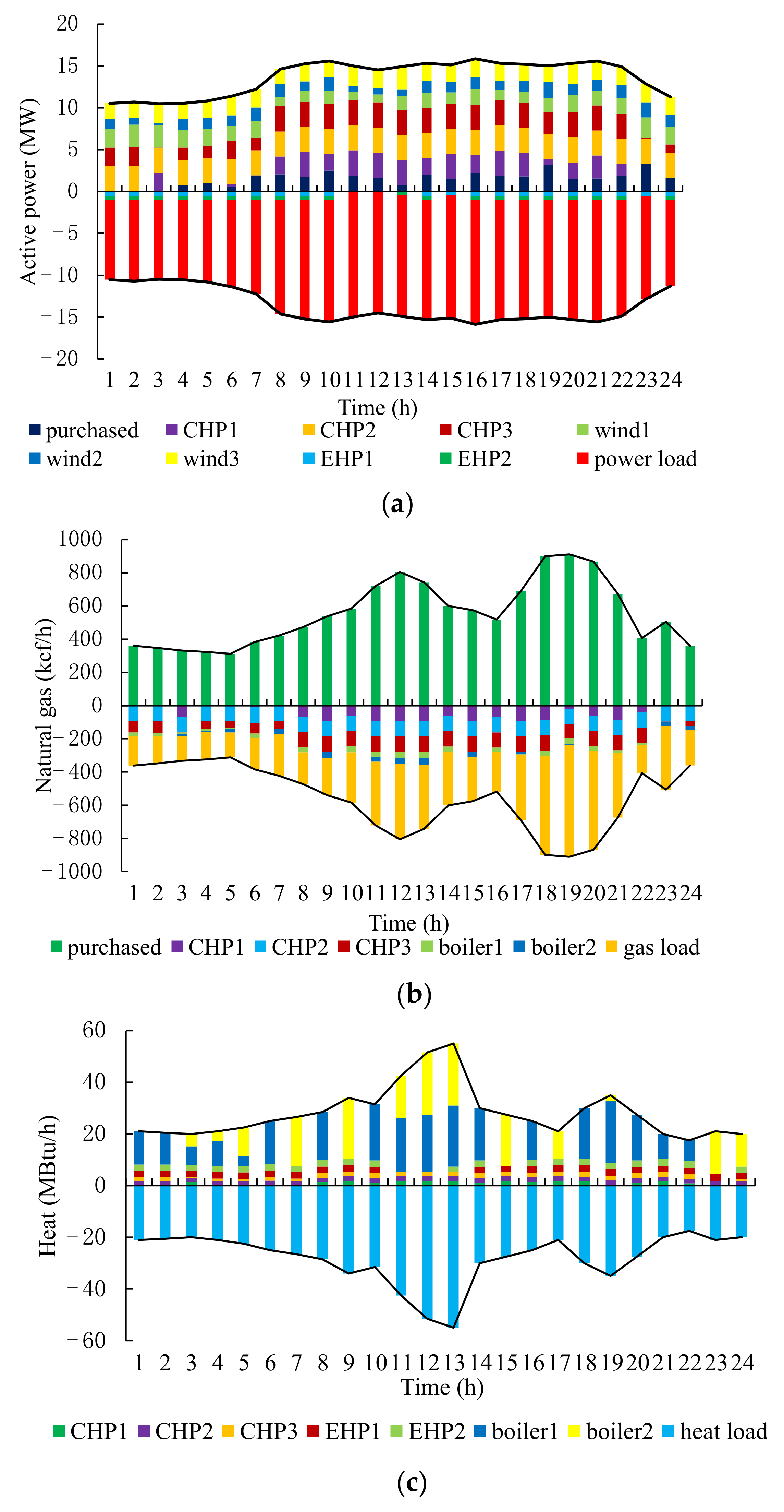
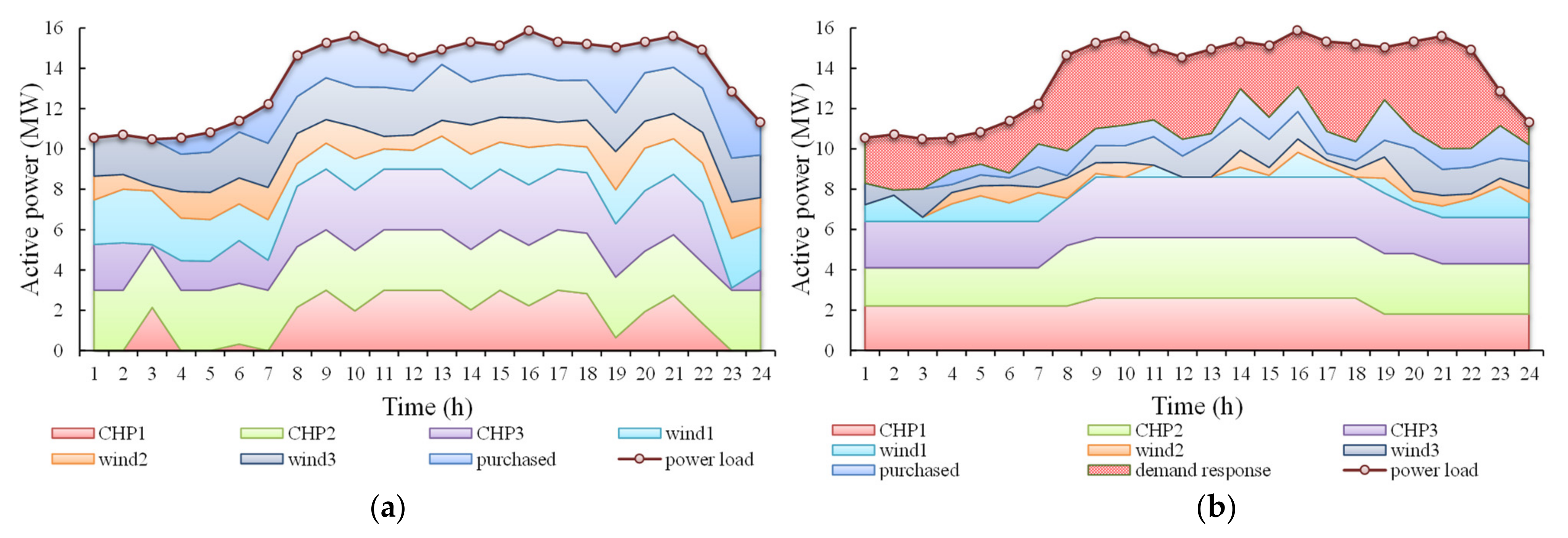
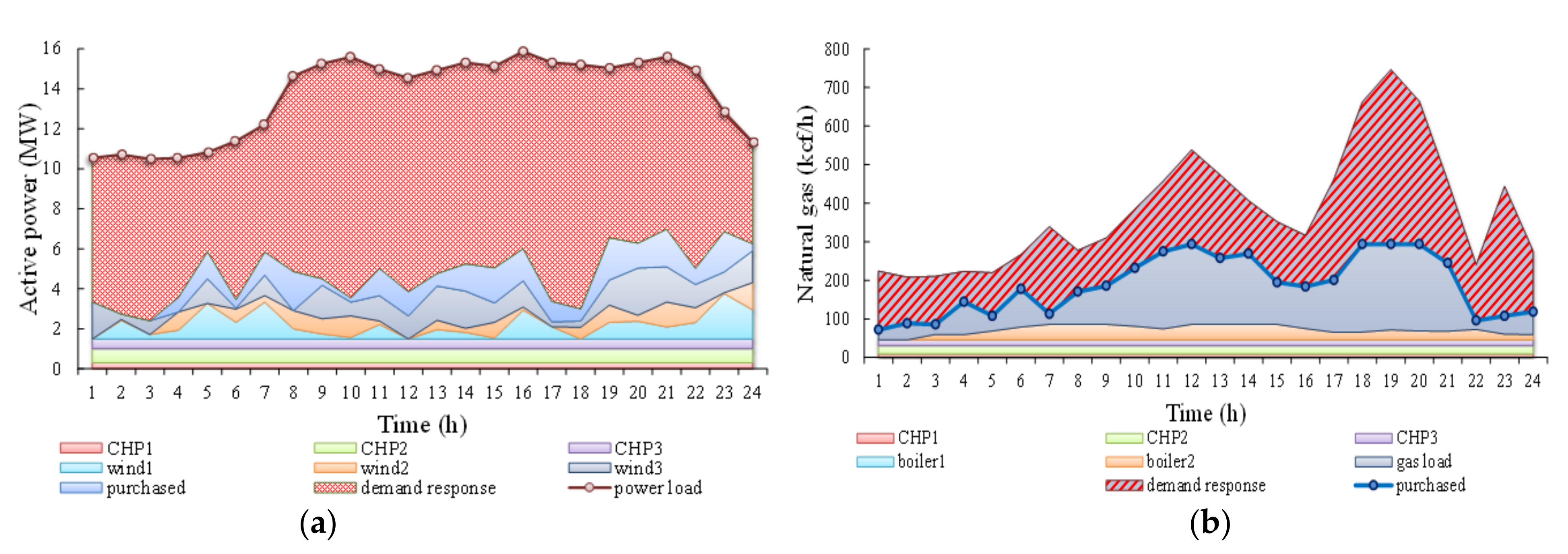
4.1. The Operation of IEDS

The proposed hardening strategy is examined on a test system, which consists of IEEE 33-bus power distribution system, 19-node gas distribution system and district heating system, shown in Figure 5. The numbers without brackets in Figure 5 represent the node number, and the numbers with brackets represent the line number.

As shown in Figure 5, there are three CHP units, two EHPs, two boilers and three wind generators. In fact, the three energy systems are geographically overlapping. For convenience, Figure 5 is a schematic diagram of the wiring of three systems.

First of all, in order to facilitate the explanation of the test system, the operation of IEDS is introduced in normal state, which is the basis of fault operation. The supply of active power load, gas load and heat load are shown in Figure 6.

As shown in Figure 6, the supply and demand of IEDS are balanced at each time slot in normal operation. However, if the overhead transmission lines or underground gas pipelines are broken, the energy supply will be restricted and load demand will not be met, so an effective demand management strategy is urgently needed to alleviate the tight supply of IEDS.

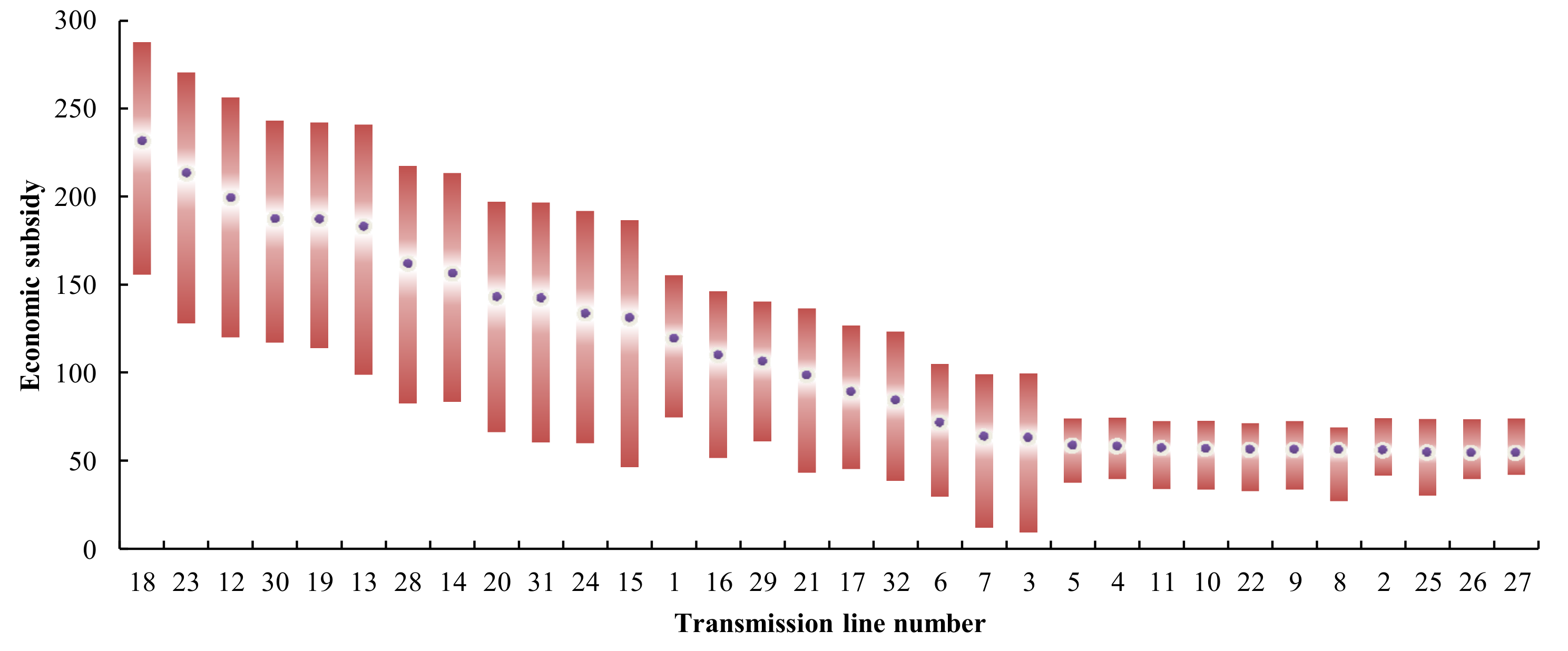
4.2. The Importance Ranking of Transmission Lines and Pipelines

After breaking transmission lines and pipelines, the amount of load demand response is calculated at each simulating fault state. This section calculates the economic subsidy caused by load demand response. The corresponding economic subsidy caused by the damaged transmission lines and pipelines is shown in

Table 2. The economic subsidy of the damaged transmission lines.

A	232.1 K	213.7 K	199.5 K	187.7 K	187.5 K	183.2 K	162.0 K	156.4 K	143.0 K	142.5 K	133.7 K	131.0 K
Line Number	18	23	12	30	19	13	28	14	20	31	24	15
B	119.4 K	109.9 K		106.4 K	98.5 K		88.9 K	84.2 K	71.4 K	63.5 K		62.8 K
Line Number	1	16		29	21		17	32	6	7		3
C	58.4 K	58.1 K	56.9 K	56.5 K	56.2 K		56.2 K	55.9 K	55.7 K	54.4 K	54.3 K	54.3 K
Line Number	5	4	11	10	22		9	8	2	25	26	27

and

Table 3. The economic subsidy of the damaged pipelines.

A	155.0 K		146.4 K		136.9 K		135.8 K		131.4 K	126.0 K
Pipeline Number	20		19		11		18		7	1
B	117.3 K	113.4 K	106.8 K	101.2 K	96.2 K	91.1 K	86.7 K	83.0 K	83.0 K	77.2 K	64.8 K
Pipeline Number	6	2	12	13	8	3	4	17	5	10	9
C	54.2 K				51.1 K				8.2 K
Pipeline Number	14				16				15

.

Then, according to the economic subsidy in each fault state, the importance of transmission lines and pipelines is ranked, which is divided into three levels. In the A-level and B-level, economic subsidy is greater than 120 K and 60 K, respectively. Economic subsidy less than 60 K is the C-level.

4.3. The Electrical Resilience Mode and Integrated Resilience Mode

In the electrical resilience mode, the surface natural disasters are simulated. In total, 100 fault scenarios are generated by non-sequential Monte-Carlo simulation, and then 5 main scenarios are obtained by scenario reduction algorithm, which are used to calculate the fault operation conditions caused by the surface natural disasters. The main scenario with the largest probability is 0.34. Transmission lines No. 6, 14, 17, 19, 29, and 30 have failed. After the failure, the power load cannot be fully supplied. Comparing the normal operation state, a demand response is required, as shown in Figure 7.

As shown in Figure 7, destruction of transmission lines results in an amount of power loads that cannot obtain electricity through outsourcing. The wind turbines are damaged due to natural disasters and the output decreases. At this time, the distribution network forms many small island grids, and CHP provides power supply to the island grids.

However, affected by the supply capacity of CHP, a certain amount of power load is still needed as a demand response resource to participate in demand management. This demand management scheme that considers the support of the natural gas system to the distribution network is called a semi-emergency scheme in this paper, and it is not necessary to use all demand response capabilities.

In the integrated resilience mode, the geological natural disasters are simulated. Similarly, 100 failure scenarios are generated and reduced to 5 main scenarios to analyze the operation of IEDS after geological natural disaster. The main scenario with the largest probability is 0.29. Transmission lines No. 7, 9, 14, 16, 20, 26, and 29 have failed. Gas pipelines No. 4, 8, 11, and 15 have failed. After the failure, not only can the power load not be fully supplied, but the natural gas is also unable to supply all the gas load due to the failure of some pipelines. The power load and gas load supply conditions are shown in Figure 8.

As shown in Figure 8, after the natural gas distribution network was destroyed by geological natural disasters, some gas pipeline failures caused a gap in natural gas supply. The red shaded part in Figure 8b is the amount of natural gas involved in gas load demand response, which is equal to the total gas load minus the largest purchased natural gas in each period.

In addition, due to the difficulty of gas supply, CHP’s ability to support power supply is extremely weak, so they all operate at a very low level of power generation. At this time, since the power load cannot get assistance from the natural gas system, almost all loads have to participate in demand management. This demand management scheme that does not consider natural gas support is called full-emergency scheme in this paper, and it is necessary to use all demand response capabilities.

It is worth mentioning that regarding the supply of heat load, in the electrical resilience mode, although pumps cannot provide heat due to insufficient power supply, gas can be used to provide sufficient heat through the boilers without causing heat load loss. In the integrated resilience mode, due to the failure of No. 8, 11, and 15 pipelines, No. 1 boiler cannot obtain gas for heating, and No. 2 boiler is used for heating, supplementally. Although part of the heat load is involved in demand response, it is not the focus of this paper and will not be analyzed in detail.

4.4. The Demand Management Strategy

From the above, the demand management strategy includes a semi-emergency demand management scheme and a full-emergency demand management scheme, according to the type of natural disaster. Moreover, the demand management strategy is based on the importance of lines and pipelines. As shown in Table 1 and Table 2, the failure of each transmission line and gas pipeline corresponds to a certain economic subsidy to the load participating in the demand response. According to the semi-emergency scheme and the full-emergency scheme, the upper and lower cost limits of the corresponding demand management for each failure transmission line and gas pipeline can be obtained, as shown in Figure 9 and Figure 10.

As shown in Figure 9 and Figure 10, according to the faults caused by natural disasters generated by non-sequential Monte-Carlo simulation, the economic subsidies for demand management caused by the failure of various transmission lines and gas pipelines fluctuate relatively widely. Therefore, the demand management strategy proposed in this paper can obtain the optimal demand management cost according to the failure situation, which can ensure that IEDS can not only improve the resilience, but also have a lower operating cost.

5. Conclusions

IEDS is an efficient, clean and sustainable energy system. However, increasingly frequent natural disasters pose a severe threat to the security of IDES. Hence, this paper studies demand management for IEDS to improve resilience against extreme events. The demand management strategy includes a semi-emergency demand management scheme and a full-emergency demand management scheme, according to the resilience mode. The strategy generation process is divided into three stages. In short, combined with component generic fragility curves, through the non-sequential Monte-Carlo simulation method and the scene reduction algorithm, the main scene of the failure caused by the natural disaster is simulated, and then according to the importance ranking of transmission line and gas pipeline the demand management economic subsidy costs under different failure situations are obtained. The main conclusions are summarized as follows:

(1) The proposed scheduling model of IEDS co-optimizes the electricity, natural gas and thermal energy in normal and failure operation state, which promotes efficient and sustainable energy consumption.

(2) This paper proposes a demand management strategy, which innovatively expands the traditional demand management in a power system. The demand management of the IEDS includes two parts: power demand management and gas demand management. This paper analyzes the economic subsidies for demand response in these two parts, respectively.

(3) The demand management strategy proposed in this paper can increase the resilience of IEDS and reduce the economic subsidy cost of demand management.

References

1. Wang, S.; Li, Y.; Haque, M. Evidence on the Impact of Winter Heating Policy on Air Pollution and Its Dynamic Changes in North China. Sustainability 2019, 11, 2728. [Google Scholar] [CrossRef] [Green Version]
2. Rashid, L.; Lin, L. Foreign Direct Investment in the Power and Energy Sector, Energy Consumption, and Economic Growth: Empirical Evidence from Pakistan. Sustainability 2019, 11, 192. [Google Scholar]
3. Ye, J.; Yuan, R. Integrated Natural Gas, Heat, and Power Dispatch Considering Wind Power and Power-to-Gas. Sustainability 2018, 9, 602. [Google Scholar] [CrossRef] [Green Version]
4. Wu, J.; Yan, J.; Jia, H. Integrated Energy Systems. Applied Energy 2016, 167, 155–157. [Google Scholar] [CrossRef]
5. Marnay, C.; Aki, H.; Hirose, K.; Kwasinski, A.; Ogura, S.; Shinji, T. Japan’s Pivot to Resilience: How Two Microgrids Fared after the 2011 Earthquake. IEEE Power Energy Mag. 2015, 13, 44–57. [Google Scholar] [CrossRef]
6. Che, L.; Khodayar, M.; Shahidehpour, M. Only Connect: Microgrids for Distribution System Restoration. IEEE Power Energy Mag. 2014, 12, 70–81. [Google Scholar]
7. Bie, Z.; Lin, Y.; Li, G. Battling the Extreme: A Study on the Power System Resilience. Proc. of the IEEE 2017, 105, 1253–1266. [Google Scholar] [CrossRef]
8. Mathaios, P.; Pierluigi, M. Modeling and Evaluating the Resilience of Critical Electrical Power Infrastructure to Extreme Weather Events. IEEE Systems Journal 2017, 11, 1733–1742. [Google Scholar]
9. Lei, S.; Wang, J.; Chen, C.; Hou, Y. Mobile Emergency Generator Pre-Positioning and Real-Time Allocation for Resilient Response to Natural Disasters. IEEE Trans. Smart Grid 2018, 9, 2030–2041. [Google Scholar] [CrossRef] [Green Version]
10. Wang, Z.; Chen, B.; Wang, J.; Chen, C. Networked Microgrids for Self-Healing Power Systems. IEEE Trans. Smart Grid 2016, 7, 310–319. [Google Scholar] [CrossRef]
11. Sergio, F.; Desta, Z.; Marco, R.; Carlos, M. Impacts of Optimal Energy Storage Deployment and Network Reconfiguration on Renewable Integration Level in Distribution Systems. Appl. Energy 2017, 185, 44–55. [Google Scholar]
12. Abdullahi, M.; Li, Y.; Stewart, M. Evaluating System Reliability and Targeted Hardening Strategies of Power Distribution Systems Subjected to Hurricanes. Reliab. Eng. Syst. Saf. 2015, 144, 319–333. [Google Scholar]
13. Lin, Y.; Bie, Z. Tri-level Optimal Hardening Plan for a Resilient Distribution System Considering Reconfiguration and DG Islanding. Applied Energy 2018, 210, 1266–1279. [Google Scholar] [CrossRef]
14. Shao, C.; Shahidepour, M.; Wang, X.; Wang, X.; Wang, B. Integrated Planning of Electricity and Natural Gas Transportation Systems for Enhancing the Power Grid Resilience. IEEE Trans. Power Syst. 2017, 32, 4418–4429. [Google Scholar] [CrossRef]
15. Cong, H.; He, Y.; Wang, X.; Jiang, C. Robust Optimization for Improving Resilience of Integrated Energy Systems with Electricity and Natural Gas Infrastructures. J. Mod. Power Syst. Clean Energy 2018, 6, 1066–1078. [Google Scholar] [CrossRef] [Green Version]
16. Amin, S.; Ali, R. An Integrated Steady-State Operation Assessment of Electrical. Natural Gas, and District Heating Networks. IEEE Trans. Power Syst. 2016, 31, 3636–3647. [Google Scholar]
17. Long, R.; Liu, J.; Shi, J.; Zhang, J. Coordinated Optimal Operation Method of the Regional Energy Internet. Sustainability 2017, 9, 848. [Google Scholar] [CrossRef] [Green Version]
18. Yao, L.; Wang, X.; Qian, T.; Qi, S.; Zhu, C. Robust Day-Ahead Scheduling of Electricity and Natural Gas Systems via a Risk-Averse Adjustable Uncertainty Set Approach. Sustainability 2018, 11, 3848. [Google Scholar] [CrossRef] [Green Version]
19. Carlos, M.; Pedro, S. Integrated Power and Natural Gas Model for Energy Adequacy in Short-Term Operation. IEEE Trans. Power Syst. 2015, 30, 3347–3355. [Google Scholar]
20. Dupacová, J.; GroWe-Kuska, N.; RoMisch, W. Scenario Reduction in Stochastic Programming an Approach Using Probability Metrics. Mathe. Program. 2003, 3, 493–511. [Google Scholar] [CrossRef]
21. Ding, T.; Lin, Y.; Li, G.; Bie, Z. A New Model for Resilient Distribution Systems by Microgrids Formation. IEEE Trans. Power Syst. 2017, 32, 4145–4147. [Google Scholar] [CrossRef]
22. He, C.; Wu, L.; Liu, T.; Shahidehpour, M. Robust Co-Optimization Scheduling of Electricity and Natural Gas Systems via ADMM. IEEE Trans. Sustain. Energy 2017, 8, 658–670. [Google Scholar] [CrossRef]
Figure 1. The typical surface natural disaster and geological natural disaster. (a) Satellite cloud picture of "Sangmei" typhoon; (b) Satellite telemetry picture of Wenchuan Earthquake.
Sustainability 14 00005 g001
Figure 2. The generic fragility curves. (a) The fragility curve of overhead transmission line under typhoon; (b) The fragility curve of underground gas pipeline under earthquake.
Sustainability 14 00005 g002
Figure 3. The framework of the demand management strategy.
Sustainability 14 00005 g003
Figure 4. The piecewise linearization of nonlinear function.
Sustainability 14 00005 g004
Figure 5. The integrated energy distribution system.
Sustainability 14 00005 g005
Figure 6. The supply of load in normal state. (a) The supply of active power load; (b) The supply of gas load; (c) The supply of heat load.
Sustainability 14 00005 g006
Figure 7. The power load supply situation. (a) The power load supply situation in normal operation state; (b) The power load supply situation in failure operation state.
Sustainability 14 00005 g007
Figure 8. The power load and gas load supply situation. (a) The power load supply situation in failure operation state; (b) The gas load supply situation in failure operation state.
Sustainability 14 00005 g008
Figure 9. The economic subsidy of power demand response.
Sustainability 14 00005 g009
Figure 10. The economic subsidy of gas demand response.
Sustainability 14 00005 g010