Article

Germany’s Agricultural Land Footprint and the Impact of Import Pattern Allocation

1
Öko-Institut e.V., Rheinstraße 95, 64295 Darmstadt, Germany
2
Center for Environmental Systems Research, University of Kassel, Wilhelmshöher Allee 47, 34109 Kassel, Germany
3
Institute of Economic Structures Research (GWS), Heinrichstr. 30, 49080 Osnabrück, Germany
*
Author to whom correspondence should be addressed.
Sustainability 2022, 14(1), 105; https://doi.org/10.3390/su14010105
Submission received: 27 November 2021 / Revised: 17 December 2021 / Accepted: 20 December 2021 / Published: 23 December 2021

Abstract

:
Footprints are powerful indicators for evaluating the impacts of a country’s bioeconomy on environmental goods, both domestic and abroad. We apply a hybrid approach combining a multi-regional input-output model and land use modelling to compute the agricultural land footprint (aLF). Furthermore, we added information on land-use change to the analysis and allocated land conversion to specific commodities. Using Germany as a case study, we show that the aLF abroad is 2.5 to 3 times larger compared to impacts within the country. When allocating land conversion of natural and semi-natural land-cover types in 2005 and 2010 to import increases by Germany, conversion rates were found to be 2.5 times higher than for the global average. Import increases to Germany slowed down in 2015 and 2020, reducing land conversion attributed to the German bioeconomy as well. Our results indicate that looking at a static import pattern is not sufficient to draw a realistic picture of the land footprint of a country. For a more detailed assessment that also considers temporal dynamics and impacts of biomass use and trade, our newly developed set of indicators also captures changes of import patterns over time. The case study shows that our enhanced land footprint provides clear and meaningful information for policymakers and other stakeholders.

1. Introduction

Biomass is the central basis for human life. It is used as food and feed but also for material and energy uses. However, the steadily increasing global consumption of biomass has negative impacts on numerous environmental goods and ecosystem functions [1,2,3]. The concept of bioeconomy (BE) encompasses agriculture, forestry, and fisheries. It aims to avoid negative impacts of biomass uses and to promote positive ones [4,5,6], especially in the context of the overarching sustainable development goals (SDGs) [7,8]. To ensure that the sustainability claim of the BE does not remain an empty phrase, it is important to monitor and document its impacts in an adequate way [9,10].
Such BE monitoring initiatives are in progress. The Joint Research Centre (JRC), e.g., works on indicators derived from the objectives of the EU bioeconomy strategy [11,12]. The Food and Agricultural Organization (FAO) has developed a methodology to assist countries and stakeholders in developing and monitoring a sustainable BE, including the selection of relevant indicators at the territorial and the product level [13]. The footprint methodology is an established approach to account for environmental impacts of human consumption both domestically and in other world regions via biomass trade. Footprint studies cover a wide range of topics such as water [14], greenhouse gas emissions [15], and land appropriation. The land footprint of a country typically determines the amount of agricultural and forested land occupied to produce the biomass consumed within that country (e.g., [16,17,18]). Bruckner et al. [19] conclude in their review on land-flow accounting methods that combining elements from environmental-economic accounting (e.g., economic input-output tables) and physical accounting (e.g., agricultural production data) is most suitable for a robust and transparent assessment of land footprints associated with global biomass flows.
In Germany, a first overview on essential traits and trends of the German BE in the national and international context has been provided by Bringezu et al. [20]. Building on that work, Bringezu et al. [21] provided a comprehensive analysis of past and projected resource and climate footprints of the German BE. This covers economic, social, and environmental impacts, including the use of agricultural and forestry biomass, value added, employment, greenhouse gas emissions, water withdrawals, and impacts from agricultural land use.
Earlier work from Fischer et al. [22] for Germany and the EU28 tracked food and non-food products from the production area to the consumer. They highlighted the increasing land demand of livestock-based diets compared to crop-based diets and the growing importance of the non-food sector using data covering the period from 2000 to 2010.
Up to now, most land-footprint analyses have concentrated on the amount of land occupation and neglected the contribution of different drivers to the conversion and loss of natural ecosystems (e.g., increasing agricultural activities in exporting regions). Specifically for agricultural land use, the conversion of natural and semi-natural land is the most important impact. As well, other aspects including habitat fragmentation and isolation as well as intensification and overexploitation have negative impacts on ecosystem functions and biodiversity [23,24,25,26]. These negative impacts include soil erosion and loss of soil fertility [27], changes in precipitation patterns [28], and greenhouse gas emissions [29].
In order to overcome this research gap, we have developed the enhanced agricultural land footprint (aLF) as a new method to provide a more comprehensive picture on the pressures on land resources caused by biomass consumption, especially in exporting regions. It accounts for both land occupation and land conversion associated with a country’s domestic consumption and export use considering cropland and grassland as the main land use categories. A first application is described in Bringezu et al. [21] where we embedded the aLF in a comprehensive monitoring of the German BE. This article gives a detailed description of the aLF method. Further, we apply the new method in a case study for assessing the global agricultural footprint of the German BE. We focus on three main questions:
(i)
How much agricultural land is used globally for the German bioeconomy and for which crops in which region of the world?
(ii)
To what extent are natural and semi-natural land areas converted to agricultural land due to the German bioeconomy?
(iii)
How much do changes of import patterns affect the results when including them in the calculation of aLF?

2. Materials and Methods

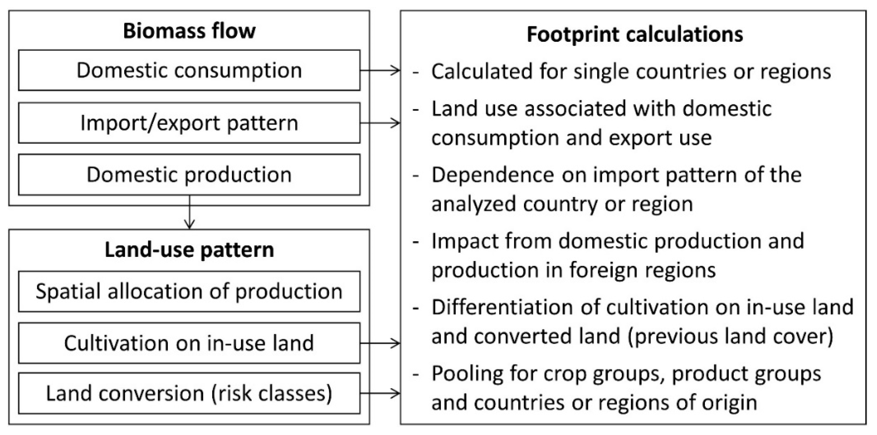
2.1. Overview of the Footprint Method

The footprint method introduced in this article combines global economic modelling and global land use modelling (Figure 1), following three steps:
  • Biomass flows between countries/regions are derived from the multi-regional input-output (MRIO) model that is based on EXIOBASE.
  • Domestic crop production of each country/region serves as input to the global land use model LandSHIFT [30]. LandSHIFT calculates the spatial pattern of agricultural land use (cropland, grassland) and additional conversion of natural and semi-natural land to agriculture.
  • The footprint calculation is carried out for a single country or region based on the results of the MRIO model and LandSHIFT.
The analysis considers domestic consumption of biomass and biomass exports due to consumption abroad as an important part of domestic value added of the country or region under analysis. Furthermore, the change in import patterns is included in the footprint analysis. The results allow for an aggregation at different levels: domestic production and production in foreign regions, land in use and land converted to cropland or grassland, differentiated by previous land cover, crop groups, product groups, and countries or regions of origin.
Our study builds on the bioeconomy definition used by the German BE policy [31] that includes the sectors agriculture, forestry and fishery; biomass-using manufacturing sectors; wood-based construction; biobased energy production; and restaurant services. BE is studied here as a part of the whole economy. For selected bio-based products, the complete life-cycle is analyzed. According to EXIOBASE, we include the crop classes paddy rice, wheat, cereal grains nec (not elsewhere classified), plant-based fibers, oil seeds, vegetables/fruits/nuts, sugar cane/sugar beet, and crops nec. In addition, soy bean and oil palm (part of oil crops), cotton (part of plant-based fibers) and fodder crops were modeled separately. Further, we distinguish 44 countries and 5 “rest-of-the-world” regions (see details below and in appendices in [21]).

2.2. Biomass Flows

The MRIO model with global coverage is based on EXIOBASE 3.4, released in July 2018, which covers the years from 1995 to 2011. Based on a variety of statistical sources, stretching from SNA data by EUROSTAT to bio-physical data by FAOSTAT, this historical database has been now-casted for the years from 2012 to 2018. To project the monetary as well as the (bio-) physical spheres of the MRIO model up to 2020 again a variety of sources has been applied: The per capita crop and per capita livestock demand are projected to follow the current trends as formulated in SSP2 [32,33]. Socio-economic and GDP trends have been taken from UN and OECD calculations respectively [34,35]. For Germany, the development of a long-term trend scenario until 2030 was based on statements of various German public institutions [36]. The two inhouse models PANTA RHEI and GINFORS helped to transfer the business-as-usual pathway into environmentally extended-IO model results on a national, multinational, and global level (see further details in [21]).
By analyzing the international supply chains, this updated and projected MRIO model for the years from 1995 to 2020 allows to trace back any national final demand to the biomass flows contained directly and indirectly, differentiated for originating countries/regions.

2.3. Global Land-Use Patterns

The spatial allocation of cropland and grassland was simulated with the land-system model LandSHIFT [30,37]. The model operates on a global raster with a cell size of 5 arc min (=9 × 9 km at the Equator). Information on biomass productivity used for identifying suitable cells for agriculture were provided by the vegetation model LPJmL [38]. LandSHIFT calculates land-use maps for the years between 1995 and 2020 by merging remote sensing data on land cover [39,40] with national statistical data from FAOSTAT [41] on crop cultivation and grazing [21].

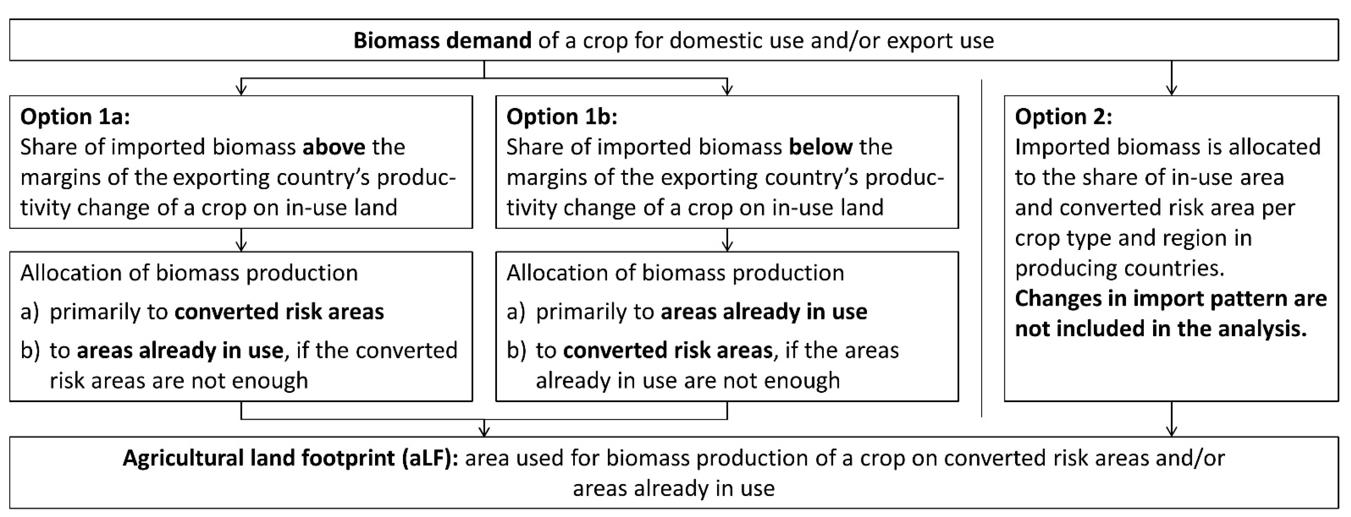
2.4. Footprint Calculations

The agricultural land footprint (aLF) of a country includes cropland and grassland areas utilized to produce commodities consumed domestically or exported which are partly or fully made from biomass. In order to calculate the aLF for a specific country, biomass flows and global land-use patterns were combined to determine the spatial extent and location of crop cultivation for domestic biomass production and imports. Global aLF is the sum of global land use driven by the biomass demand of the world’s population.
The agricultural land footprint considers traits of the occupied area to estimate footprint impacts on ecosystem services and biodiversity through habitat loss. The ecosystem areas associated with habitat loss from conversion into agricultural land were compiled into nine risk area classes: (1) primary forest, (2) biodiverse forest, (3) biodiverse grassland, (4) other biodiverse land fusing information on biodiversity with land cover, (5) peatland, (6) wetlands, (7) forest, (8) unused grassland not used for grazing by LandSHIFT, and (9) used grassland (see references in [21]). Areas that remain in agricultural use, as cropland or as grassland, and conversion of settlements are assumed to have a much lower impact on ecosystem services and biodiversity. Further, established protected areas were excluded from conversion to agricultural land.
The conversion of land is calculated for five-year periods as the rate of complete risk area conversion. This rate is influenced by changes in productivity in the country of origin and by changes in imports of the importing country. In cases where imports increase proportionally with the exporting country’s production on land in use (e.g., due to yield increase), no conversion is allocated to the footprint of the importing country’s BE. If growth rates of imports exceed those of productivity, additional land for agricultural cultivation is established through conversion of risk areas and allocated to imports of the importing country (see Option 1a and 1b in Figure 2).

2.5. Case Study Germany

In our case study, the aLF is calculated as the agricultural land used for biomass production for the domestic consumption and export use of the German BE. For comparison, the aLF is also computed as a global average. The aLF is expressed as area used or area used per person. We calculated the aLF for Germany as the sum of all crop groups and regions as well as disaggregated by regions, crop groups, and product groups, applying Option 1a and 1b in Figure 2.
To analyze the effect of changes in import patterns, the allocation of land use was also calculated without accounting for these changes (Option 2 in Figure 2). In this case, the share of area in use and risk area converted by crop type and region in producing countries was directly allocated to the imported biomass. Our study includes four combinations:
  • Analysis related to import changes (ric) and domestic use (aLFdom, ric);
  • Analysis related to import changes (ric) and export use including re-export (aLFexp, ric);
  • Analysis not related to import changes (not-ric) and domestic use (aLFdom, no-ric);
  • Analysis not related to import changes (not-ric) and export use including re-export (aLFexp, not-ric).

3. Results

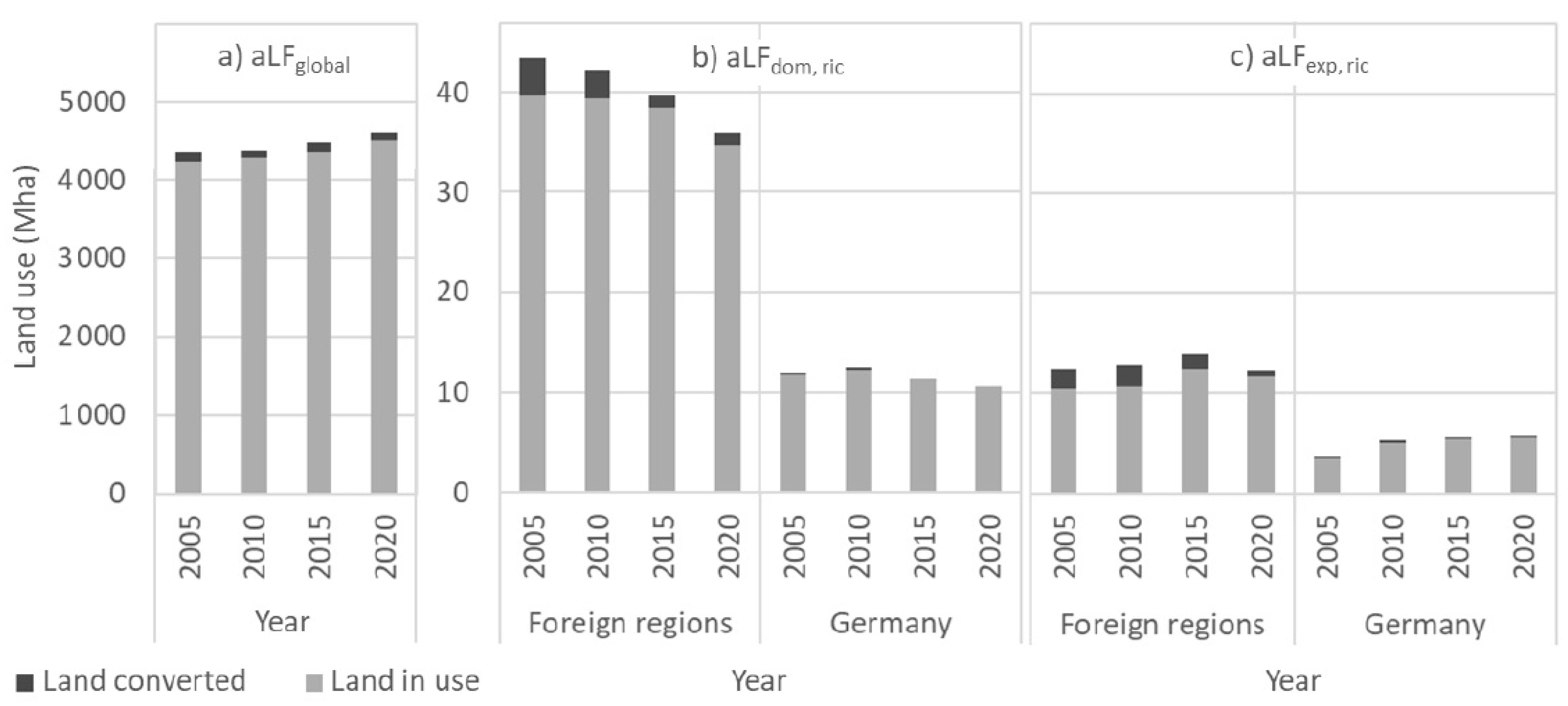
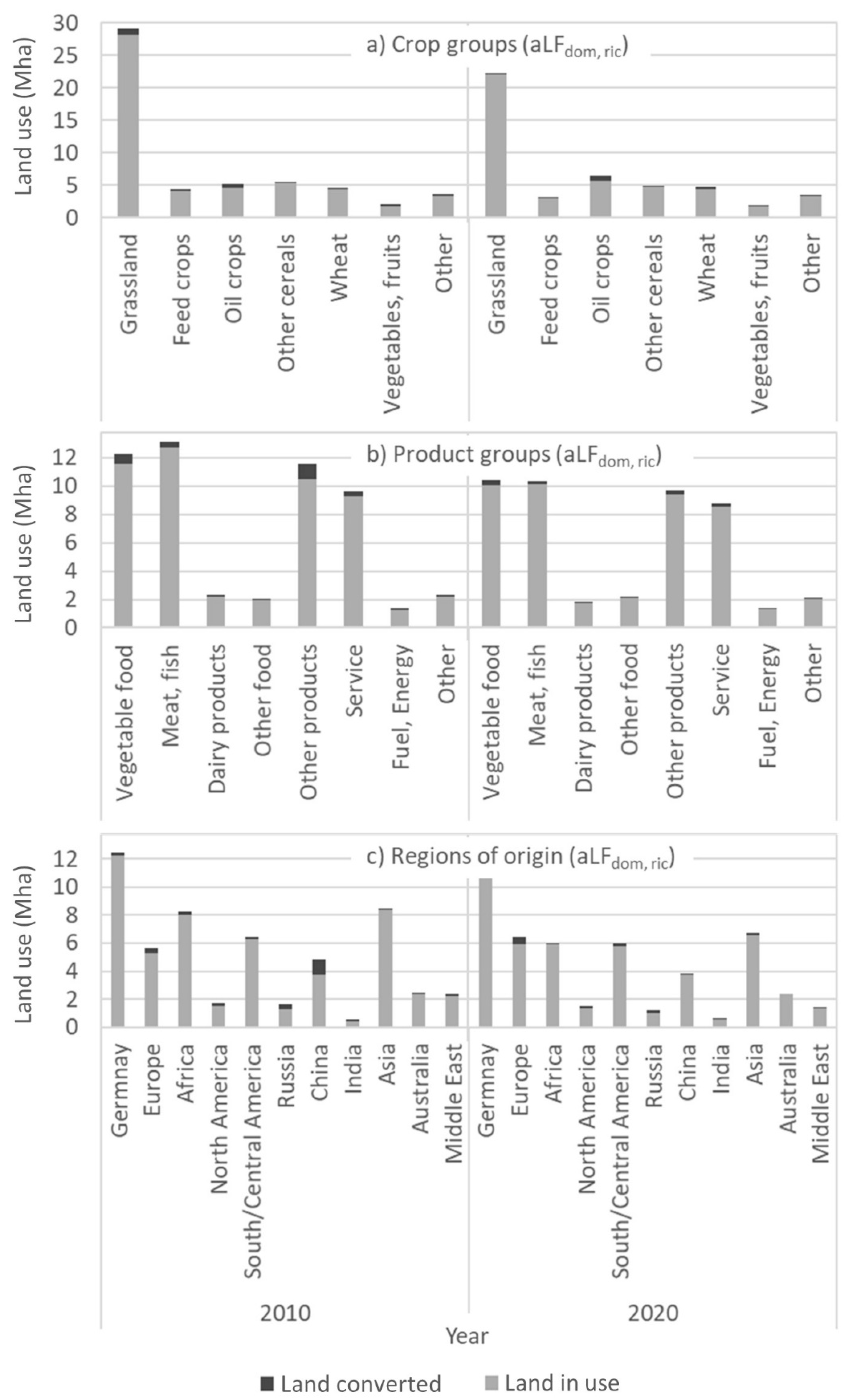
3.1. Land Used by the German Bioeconomy

As shown in Figure 3a, the agricultural land used to meet global biomass consumption is projected to increase from 4.36 billion ha in 2005 to 4.61 billion ha in 2020. The majority of the required land is land already in use, while about 20 Mha annually (93 to 115 Mha over each five-year period) additional land is newly converted. In contrast, German consumption is projected to gradually occupy less agricultural land until 2020 (Figure 3b). In particular, this is the case for agricultural land in regions that export biomass to Germany (−17% from 2005 to 2020), while the decrease of land for agricultural production in Germany is less pronounced (−11%; Figure 3b). German exports account for a smaller share of the aLF compared to German domestic consumption (Figure 3c). The area of newly converted land is decreasing over time, both for German domestic consumption and export use.
The aLF clearly shows how the German BE relies on a high demand for land abroad. The agricultural area in Germany occupies about 17 Mha for domestic consumption and export use. But there are 56 Mha in other world regions in 2005 and 48 Mha in 2020 (Figure 3b,c) supplying BE goods for Germany. Thus, German BE land requirements in foreign regions are about 3 times higher than domestic land use.
For the time periods 2010 (including from 2006 to 2010) and 2020 (including from 2016 to 2020), Figure 4 shows land use differentiated by crop groups, product groups and regions of origin. The shares of land converted of total land use are again relatively low compared to total land used for biomass production (see also Figure 3b). In addition to production in Germany and Europe, biomass is produced to a large extent in Asia, Africa, and South/Central America (Figure 4c). Within the German BE, biomass is primarily used for food production as vegetable food, meat and fish, dairy products and other food (Figure 4b). The total use of biomass for food is even larger as the group of other products and services include also food uses, such as canteen meals and hotel services. Grassland and feed crops for livestock dominate land use for crops with more than 60% in 2010 and almost 55% in 2020 (Figure 4a).

3.2. Land Converted by the German Bioeconomy

Globally, conversion of risk areas due to German consumption of agricultural products fluctuates between 19 and 23 Mha/a from 2005 to 2020 (Figure 5a). This corresponds to a per capita value of 27 to 34 m2/(person*a). In most cases, used grassland, unused grassland and forest areas are affected. Particularly sensitive areas such as primary forest and highly biodiverse land categories are converted much less with about 0.7 Mha/a and 1 m2/(person*a), respectively.
However, in the past land conversion driven by German domestic consumption showed higher values of 0.74 Mha/a (90 m2/(person*a)) in 2005 and 0.57 Mha/a (71 m2/(person*a)) in 2010 (Figure 5b). At that time, the conversion rate per capita was about 2.5 times higher than the global mean in 2005 and 2010 and conversion occurred almost exclusively in regions abroad. Moreover, between 2001 and 2010, land conversion of particularly sensitive areas like biodiverse forests, biodiverse grasslands and wetlands was significantly higher compared to global patterns (Figure 5a,b). In Germany, only a comparably small amount of used grassland was converted to cropland. In the following decade, however, land use change related to consumption in Germany decreased significantly and reached values of 0.27 Mha/a (31 m2/(person*a); Figure 5b). A similar pattern can also be observed for German exports and re-exports (Figure 5c) with a land conversion rate in foreign regions of about 0.40 Mha/a in 2005 and 2010 decreasing to 0.10 Mha/a in 2020.

3.3. Allocation of Changes of Import Patterns

The calculation of Germany’s aLF considers changes of the import pattern related to the German domestic and export use of agricultural products (Option 1 in Figure 2). If changes in import patterns are not considered (Option 2 in Figure 2), land conversion allocated to the German BE changes significantly. In 2005 and 2010 we see that less land conversion, especially in foreign regions, is assigned to consumption in Germany (Figure 5d). For German export use, the differences between the two approaches are even more pronounced (Figure 5e). Furthermore, if import changes are ignored, considerably less conversion of particularly sensitive areas is detected compared to the analysis related to import changes (Figure 5d compared to Figure 5b,e compared to Figure 5c).

4. Discussion

The production of agricultural commodities for domestic and foreign markets occupies land and drives land conversion, while the locations of consumption and production are often separated geographically. Environmental footprints aim to visualize impacts of consumption and related trade on different environmental dimensions such as GHG emissions, biomass, land use and water use. They can serve as an important indicator for bioeconomy monitoring that aims at fostering a more sustainable development within planetary boundaries (e.g., [9,42]) with a focus on specific commodities, countries, or sectors [20,21,22].
Our analysis combines MRIO data on biomass flows and global land use modelling to assess changes in land use presumably triggered by changes in consumption, agricultural production and global trade. The modelled results can be compared with other backward-looking assessments based on the combination of trade statistics and satellite data (e.g., [43]). In contrast to other analyses that put specific commodities into perspective [44], or focus on a specific type of land use change (e.g., deforestation [45]), this paper analysis the whole spectrum of conversions across different land use categories related to the BE in Germany. Earlier work with a focus on Germany included a higher level of detail for agricultural commodities but was less detailed regarding the quality of land use data and land-use changes [22].

4.1. Land Used by the German Bioeconomy

Three general observations can be made regarding the aLF of the BE in Germany. The first observation is that the aLF abroad is 2.5 to 3 times larger than the aLF in Germany. This is the case for domestic use and somewhat less pronounced for export use. The total agricultural area associated with the BE in Germany, as domestic use and export use, amounts to 65 to 71 Mha, with about 15 to 17 Mha of agricultural land in Germany and 48 to 56 Mha of agricultural land abroad. This clearly documents the strong dependency of German BE from agricultural land abroad.
Fischer et al. [22] also report high values of land use abroad serving the demand for agricultural products in Germany. In 2010, one third of the German demand for agricultural commodities was met domestically, two thirds from abroad. In the case of grassland use, land use abroad was about three times higher than domestic grassland use. Their estimate of land occupied in Germany domestically of 12 Mha of arable land and 4.5 Mha of grassland corresponds with the results of this study. For land occupied abroad for imports to Germany for domestic consumption in 2010, we computed about 42 Mha, and Fischer et al. a slightly lower amount of 39 Mha. However, the share of cropland and grassland differ. In our results the virtual imports are 40% cropland and 60% grassland, whereas Fischer et al. reports 62% cropland and 38% grassland. These differences are probably a result of the allocation procedure of grassland for feeding livestock in producing countries or regions, but also depend on the underlying assumptions regarding crop yields, the selection of production sites, especially in larger regions, and the release version of the EXIOBASE database applied in the two studies.
It should also be emphasized that high shares of 55% (2020) to 60% (2010) in the aLF of domestic consumption can be allocated to the consumption of animal products (grassland, feed crops). For this share of land use, the consumption of meat plays a significantly greater role than the consumption of dairy products. Comparable shares were mentioned in [28], also using a hybrid approach model, stressing the power of MRIO in combination with land use modelling to relate consumption patterns to crop production.
The second observation is that the aLF abroad for domestic use decreases from 43 Mha in 2005 to 36 Mha in 2020. This effect can be explained by increasing crop yields in exporting countries in combination with a comparable low increase of imports by Germany for domestic use [20,21], see also [22]. The trend of a decreasing aLF becomes particularly clear in regions of origin such as Asia or Africa. For re-exports, the aLF remains more or less constant, as improvements due to crop yield increases achieved abroad are offset by an increase in the absolute quantity for re-exports. At the same time, at the global level the development of the aLF shows the opposite pattern: land use by the BE increases by 6% from 2005 to 2020 (0.3% per year). This is due to the fact that consumption per person and global population increase to a greater extent than crop yields, cf. [21].
The third observation relates to our finding that the German BE was associated with a high conversion of sensitive ecosystems to arable land in exporting regions, especially in the years between 2005 and 2010. This observation is discussed in more detail in the next section.

4.2. Land Converted by the German Bioeconomy

Bracco et al. [10] reviewed territorial and product-level indicators from various bioeconomy monitoring approaches. They identified a lack of consideration of import patterns as a major shortcoming in monitoring approaches. Our approach overcomes this shortcoming. It combines data on imports of the consuming country with data on conversion in the country of origin for assessing the impact of the BE on the loss of natural and semi-natural ecosystems. The aLF indicator is applicable for all countries and regions covered in the underlying data. We show that for Germany domestic land use changes related to the BE were rather small. This is due to national laws and regulations preventing sensitive areas from being converted to agricultural land. An exception is the conversion of grassland to arable land, particularly before 2010 as a result of an increased cultivation of bioenergy substrates [46]. This conversion was prevented through restrictions of grassland conservation introduced by ‘greening measures’ under the EU’s common agricultural policy (CAP) in 2015 [47].
In 2005 and 2010, already a large area share abroad served to fulfil biomass demand in Germany, and biomass imports increased further. The calculated aLF documents this development and allocates converted sensitive areas in producer countries to German imports. In 2005 and 2010, per-capita land conversion abroad allocated to Germany is 2.5 times higher than the global average. In particular sensitive areas, such as biodiverse land, unused grassland and forest, are more affected than at global average. Growth of imports to Germany slowed down in 2015 and 2020, reducing land conversion attributed to the German bioeconomy compared to the global average. Land categories most affected by conversion were used grasslands and, to a smaller degree highly biodiverse areas, wetlands and unused grassland.
Global trade shifts environmental burdens (i.e., loss of biodiversity and ecosystem functions) associated with the German BE to geographically distant regions [48]. With the aLF, we present an indicator for assessing these losses quantitatively. There are limitations to the interpretation of these results related to the quality of data that need to be acknowledged. For example, the conversion of biodiverse forest can be associated with stronger negative effects on biodiversity than the conversion of forest with lower biodiversity value. The actual impact of the loss of sensitive areas (e.g., with high biodiversity) also depends on the region of origin. In tropical regions the loss of such areas can result in stronger negative impacts compared to areas in other regions [49]. This is due to the underlying data that provide a consistent layer of information regarding biodiversity across regions but do not capture the specific value of an area from a regional perspective. Another example relates to the risk of losing soil fertility through erosion that is significantly higher on steep slopes compared to flat terrain. Adding such a level of detail for more detailed assessments of risks to soil fertility would require a higher resolution of modelling and land allocation. Bringezu et al. [21] provided an example on how the method described in this article can be applied also to assess the water footprint of the BE through the integration of climate and land-use data at watershed level. The methodological approach of the aLF presented her can thus be adapted also for an assessment of other ecosystem functions.

4.3. Allocation of Changes of Import Patterns

To understand the sensitivity of the aLF to different allocation schemes of changes of import patterns, the indicator was calculated with (Option 1) and without covering changes of import patterns (Option 2). Option 2 resulted in significantly less land conversion allocated to the German BE and also in less sensitive land use types affected, compared to Option 1. The difference is more pronounced if import increases are higher. However, if imports remain stable or even decrease, the allocated land conversion is assumed to decrease to zero under Option 1. The sensitivity analysis shows that neglecting the change of import patterns leads to inaccurate results. This is because import patterns are a key driver of land-use change, as we computed in the aLF. In the case that a qualitative change is integrated in the footprint (e.g., change of species richness, change of soil fertility or change of carbon stock), the change of import patterns should be included in the calculation as well (or at least its impact should be tested).
The presented aLF enables us to assess the magnitude of land use in connection with biomass use in a country. As the aLF also considers land conversion, it additionally allows for an assessment of the quality of land use change. Therefore the indicator provides an approach to document the extent of the loss of sensitive areas domestically and abroad that is related to the development of the BE in a country.

5. Conclusions

For monitoring the bioeconomy’s environmental footprint on domestic land use and abroad, there is the need for ready-to-use indicators that provide clear and meaningful information for policymakers and other stakeholders.
We present the agricultural land footprint (aLF) as an approach that combines global trade data and modelling of historic land-use, and it allocates biomass use and trade to observed land use and land conversion. The indicator provides a quantitative estimate of land use and land conversion of specific commodities caused by biomass use. We illustrate the approach by using a case study of the German bioeconomy and highlighting Germany’s responsibility for the conversion of natural and semi-natural land in exporting countries between 2005 and 2010 and its decrease until 2020.
Our results show that the current import pattern itself is not sufficient to draw a realistic picture of the land footprint of a country. Therefore, our indicator additionally captures changes of import patterns to better assess dynamics and impacts of biomass use and trade. The methodological approach of the aLF presented in this article can be applied to any country and region covered in EXIOBASE. It can be adapted also for an assessment of other ecosystem functions, such as water or soil fertility.

Author Contributions

Conceptualization, K.J.H., F.W. and H.B.; methodology, K.J.H., F.W. and H.B.; validation, K.J.H., F.W. and H.B.; formal analysis, M.D. and C.L.; investigation, K.J.H.; data curation, F.W. and R.S.; writing—original draft preparation, K.J.H., S.G., H.B. and R.S.; visualization, S.G. All authors have read and agreed to the published version of the manuscript.

Funding

This research was funded by the German Federal Ministry of Education and Research (BMBF) within the framework of the SYMOBIO project (number 031 B0281A).

Institutional Review Board Statement

Not applicable.

Informed Consent Statement

Not applicable.

Data Availability Statement

The data presented in this study are available on request from the corresponding author.

Acknowledgments

We thank all our colleagues for the inspiring collaboration in the SYMOBIO project, in particular our coordinator Stefan Bringezu from CESR/University of Kassel.

Conflicts of Interest

The authors declare no conflict of interest. The funders had no role in the design of the study; in the collection, analyses, or interpretation of data; in the writing of the manuscript; or in the decision to publish the results.

References

  1. IPBES. Global Assessment Report on Biodiversity and Ecosystem Services of the Intergovernmental Science-Policy Platform on Biodiversity and Ecosystem Services; Brondizio, E.S., Settele, J., Díaz, S., Ngo, H.T., Eds.; IPBES Secretariat: Bonn, Germany, 2019. [Google Scholar]
  2. WBGU. Landwende im Anthropozän: Von der Konkurrenz zur Integration. Berlin. 2020. Available online: https://www.wbgu.de/fileadmin/user_upload/wbgu/publikationen/hauptgutachten/hg2020/pdf/WBGU_HG2020_ZF.pdf (accessed on 22 November 2021).
  3. Moore, J.C. The re-imagining of a framework for agricultural land use: A pathway for integrating agricultural practices into ecosystem services, planetary boundaries and sustainable development goals. Ambio 2021, 50, 1295–1298. [Google Scholar] [CrossRef]
  4. European Commission. A Sustainable Bioeconomy for Europe: Strengthening the Connection between Economy, Society and the Environment: Updated Bioeconomy Strategy; European Commission: Brussels, Belgium, 2018. [Google Scholar]
  5. Meyer, R. Bioeconomy Strategies: Contexts, Visions, Guiding Implementation Principles and Resulting Debates. Sustainability 2017, 9, 1031. [Google Scholar] [CrossRef] [Green Version]
  6. Kuosmanen, T.; Kuosmanen, N.; El-Meligli, A.; Ronzon, T.; Gurria, P.; Iost, S.; M’Barek, R. How Big Is the Bioeconomy? Reflections from an Economic Perspective; Publications Office of the European Union: Luxembourg, 2020. [Google Scholar]
  7. Heimann, T. Bioeconomy and SDGs: Does the bioeconomy support the achievement of the SDGs? Earth’s Future 2019, 7, 43–57. [Google Scholar] [CrossRef] [Green Version]
  8. Linser, S.; Lier, M. The contribution of sustainable development goals and forest-related indicators to national bioeconomy progress monitoring. Sustainability 2020, 12, 2898. [Google Scholar] [CrossRef] [Green Version]
  9. O’Brien, M.; Wechsler, D.; Bringezu, S.; Schaldach, R. Toward a systemic monitoring of the European bioeconomy: Gaps, needs and the integration of sustainability indicators and targets for global land use. Land Use Policy 2017, 66, 162–171. [Google Scholar] [CrossRef]
  10. Bracco, S.; Calicioglu, O.; Gomez San Juan, M.; Flammini, A. Assessing the Contribution of Bioeconomy to the Total Economy: A Review of National Frameworks. Sustainability 2018, 10, 1698. [Google Scholar] [CrossRef] [Green Version]
  11. Giuntoli, J.; Robert, N.; Ronzon, T.; Sanchez Lopez, J.; Follador, M.; Girardi, I.; Barredo Cano, J.; Borzacchiello, M.; Sala, S.; M’Barek, R.; et al. Building a Monitoring System for the EU Bioeconomy; Publications Office of the European Union: Luxembourg, 2020; ISBN 978-92-76-15385-6. [Google Scholar]
  12. Kilsedar, C.E.; Wertz, S.; Robert, N.; Mubareka, S. Implementation of the EU Bioeconomy Monitoring System Dashboards: Status and Technical Description as of December 2020; Publications Office of the European Union: Luxembourg, 2021; ISBN 978-92-76-28946-3. [Google Scholar]
  13. Bracco, S.; Tani, A.; Çalıcıoğlu, Ö.; Gomez San Juan, M.; Bogdanski, A. Indicators to Monitor and Evaluate the Sustainability of Bioeconomy. Overview and a Proposed Way Forward. Rome. 2019. Available online: https://www.fao.org/3/ca6048en/CA6048EN.pdf (accessed on 22 November 2021).
  14. ISO 14046:2014. Environmental Management—Water Footprint—Principles, Requirements and Guidelines; International Organization for Standardization: Geneva, Switzerland, 2014. [Google Scholar]
  15. ISO 14067:2018. Greenhouse Gases—Carbon Footprint of Products—Requirements and Guidelines for Quantification; International Organization for Standardization: Geneva, Switzerland, 2018. [Google Scholar]
  16. Giljum, S.; Wieland, H.; Lutter, S.; Bruckner, M.; Wood, R.; Tukker, A.; Stadler, K. Identifying priority areas for European resource policies: A MRIO-based material footprint assessment. J. Econ. Struct. 2016, 5, 17. [Google Scholar] [CrossRef] [Green Version]
  17. Bruckner, M.; Häyhä, T.; Giljum, S.; Maus, V.; Fischer, G.; Tramberend, S.; Börner, J. Quantifying the global cropland footprint of the European Union’s non-food bioeconomy. Environ. Res. Lett. 2019, 14, 45011. [Google Scholar] [CrossRef]
  18. Liobikiene, G.; Chen, X.; Streimikiene, D.; Balezentis, T. The trends in bioeconomy development in the European Union: Exploiting capacity and productivity measures based on the land footprint approach. Land Use Policy 2020, 91, 104375. [Google Scholar] [CrossRef]
  19. Bruckner, M.; Giljum, S.; Fischer, G.; Tramberend, S. Review of Land Flow Accounting Methods and Recommendations for Further Development; German Environment Agency: Dessau-Roßlau, Germany, 2017. [Google Scholar]
  20. Bringezu, S.; Banse, M.; Ahmann, L.; Bezama, N.A.; Billig, E.; Bischof, R.; Blanke, C.; Brosowski, A.; Brüning, S.; Borchers, M.; et al. Pilotbericht zum Monitoring der Deutschen Bioökonomie; Center for Environmental Systems Research (CESR), Universität Kassel: Kassel, Germany, 2020. [Google Scholar]
  21. Bringezu, S.; Distelkamp, M.; Lutz, C.; Wimmer, F.; Schaldach, R.; Hennenberg, K.J.; Böttcher, H.; Egenolf, V. Environmental and socioeconomic footprints of the German bioeconomy. Nat. Sustain. 2021, 4, 775–783. [Google Scholar] [CrossRef]
  22. Fischer, G.; Tramberend, S.; Bruckner, M.; Lieber, M. Quantifying the Land Footprint of Germany and the EU Using a Hybrid Accounting Model; Umweltbundesamt: Dessau-Roßlau, Germany, 2017. Available online: https://www.umweltbundesamt.de/sites/default/files/medien/1410/publikationen/2017-09-06_texte_78-2017_quantifying-land-footprint.pdf (accessed on 22 November 2021).
  23. Hennenberg, K.J.; Dragisic, C.; Haye, S.; Hewson, J.; Semroc, B.; Savy, C.; Wiegmann, W.; Fehrenbach, H.; Fritsche, U.R. The power of bioenergy-related standards to protect biodiversity. Conserv. Biol. 2010, 24, 412–423. [Google Scholar] [CrossRef] [PubMed]
  24. Pereira, H.M.; Navarro, L.M.; Martins, I.S. Global biodiversity change: The bad, the good, and the unknown. Annu. Rev. Environ. Resour. 2012, 37, 25–50. [Google Scholar] [CrossRef] [Green Version]
  25. Kehoe, L.; Romero-Muñoz, A.; Polaina, E.; Estes, L.; Kreft, H.; Kuemmerle, T. Biodiversity at risk under future cropland expansion and intensification. Nat. Ecol. Evol. 2017, 1, 1129–1135. [Google Scholar] [CrossRef] [PubMed]
  26. Hasan, S.S.; Zhen, L.; Miah, M.G.; Ahamed, T.; Samie, A. Impact of land use change on ecosystem services: A review. Environ. Dev. 2020, 34, 100527. [Google Scholar] [CrossRef]
  27. Borrellia, P.; Robinsonc, D.A.; Panagosd, P.; Lugatod, E.; Yangb, J.E.; Alewella, C.; Wueppere, D.; Montanarellad, L.; Ballabiod, C. Land use and climate change impacts on global soil erosion by water (2015–2070). Proc. Natl. Acad. Sci. USA 2020, 117, 21994–22001. [Google Scholar] [CrossRef] [PubMed]
  28. Wierik, S.A.T.; Cammeraat, E.L.H.; Gupta, J.; Artzy-Randrup, Y.A. Reviewing the impact of land use and land-use change on moisture recycling and precipitation patterns. Water Resour. Res. 2021, 57, e2020WR029234. [Google Scholar] [CrossRef]
  29. Lamb, W.F.; Wiedmann, T.; Pongratz, J.; Andrew, R.; Crippa, M.; Olivier, J.G.J.; Wiedenhofer, D.; Mattioli, G.; Al Khourdajie, A.; House, J.; et al. A review of trends and drivers of greenhouse gas emissions by sector from 1990 to 2018. Environ. Res. Lett. 2021, 16, 73005. [Google Scholar] [CrossRef]
  30. Schaldach, R.; Koch, J.; der Beek, T.A.; Kynast, E.; Flörke, M. Current and future irrigation water requirements in pan-Europe: An integratedanalysis of socio-economic and climate scenarios. Glob. Planet. Chang. 2012, 94–95, 33–45. [Google Scholar] [CrossRef]
  31. Bundesministerium für Ernährungund Landwirtschaft. Fortschrittsbericht zur Nationalen Politikstrategie Bioökonomie. 2016. Available online: https://www.bmel.de/SharedDocs/Downloads/DE/Broschueren/Fortschrittsbericht-Biooekonomie.pdf;jsessionid=AA46C39D03E7ECE32D237152034228EC.live842?__blob=publicationFile&v=2 (accessed on 22 November 2021).
  32. Riahi, K.; Van Vuuren, D.P.; Kriegler, E.; Edmonds, J.; O’neill, B.C.; Fujimori, S.; Bauer, N.; Calvin, K.; Dellink, R.; Fricko, O.; et al. The Shared Socioeconomic Pathways and their energy, land use, and greenhouse gas emissions implications: An overview. Glob. Environ. Chang. 2017, 42, 153–168. [Google Scholar] [CrossRef] [Green Version]
  33. O’Neill, B.C.; Kriegler, E.; Ebi, K.L.; Kemp-Benedict, E.; Riahi, K.; Rothman, D.S.; van Ruijven, B.J.; van Vuuren, D.P.; Birkmann, J.; Kok, K.; et al. The roads ahead: Narratives for shared socioeconomic pathways describing world futures in the 21st century. Glob. Environ. Chang. 2017, 42, 169–180. [Google Scholar] [CrossRef] [Green Version]
  34. United Nations. World Population Prospects 2019: Volume I: Comprehensive Tables. 2019. Available online: https://population.un.org/wpp/Publications/Files/WPP2019_Volume-I_Comprehensive-Tables.pdf (accessed on 22 November 2021).
  35. Dellink, R.; Chateau, J.; Lanzi, E.; Magné, B. Long-term economic growth projections in the Shared Socioeconomic Pathways. Glob. Environ. Chang. 2017, 42, 200–214. [Google Scholar] [CrossRef]
  36. Lutz, C.; Becker, L.; Ulrich, P.; Distelkamp, M. Sozioökonomische Szenarien als Grundlage der Vulnerabilitätsanalysen für Deutschland: Teilbericht des Vorhabens “Politikinstrumente zur Klimaanpassung”, Dessau-Roßlau. 2019. Available online: https://www.umweltbundesamt.de/sites/default/files/medien/1410/publikationen/2019-05-29_cc_25-2019_soziooekonomszenarien.pdf (accessed on 22 November 2021).
  37. Schaldach, R.; Alcamo, J.; Koch, J.; Kölking, C.; Lapola, D.M.; Schüngel, J.; Priess, J.A. An integrated approach to modelling land-use change on continental and global scales. Environ. Modell. Softw. 2011, 26, 1041–1051. [Google Scholar] [CrossRef]
  38. Bondeau, A.; Smith, P.; Zaehle, S.; Schaphoff, S.; Lucht, W.; Cramer, W.; Gerten, D.; Lotze-Campen, H.; Müller, C.; Reichstein, M.; et al. Modelling the role of agriculture for the 20th century global terrestrial carbon balance. Glob. Chang. Biol. 2007, 13, 679–706. [Google Scholar] [CrossRef]
  39. CCI. ESA Climate Change Initiative—Land Cover Led by UCLouvain. 2017. Available online: http://maps.elie.ucl.ac.be/CCI/viewer/download.php (accessed on 22 November 2021).
  40. ESA. Land Cover CCI Product User Guide Version 2. 2017. Available online: Maps.elie.ucl.ac.be/CCI/viewer/download/ESACCI-LC-Ph2-PUGv2_2.0.pdf (accessed on 22 November 2021).
  41. FAO. FAOSTAT Database Collections. Rome. 2020. Available online: http://faostat.fao.org (accessed on 31 January 2020).
  42. Egenolf, V.; Bringezu, S. Conceptualization of an indicator system for assessing the sustainability of the bioeconomy. Sustainability 2019, 11, 443. [Google Scholar] [CrossRef] [Green Version]
  43. Winkler, K.; Fuchs, R.; Rounsevell, M.; Herold, M. Global land use changes are four times greater than previously estimated. Nat. Commun. 2021, 12, 2501. [Google Scholar] [CrossRef]
  44. Henders, S.; Persson, U.M.; Kastner, T. Trading forests: Land-use change and carbon emissions embodied in production and exports of forest-risk commodities. Environ. Res. Lett. 2015, 10, 125012. [Google Scholar] [CrossRef]
  45. European Commission. The Impact of EU Consumption on Deforestation: Comprehensive Analysis of the Impact of EU Consumption on Deforestation; European Commission: Brussels, Belgium, 2013; ISBN 9789279289262. [Google Scholar]
  46. Lüker-Jansa, N.; Simmering, D.; Otte, A. The impact of biogas plants on regional dynamics of permanent grassland and maize area—The example of Hesse, Germany (2005–2010). Agr. Ecosyst. Environ. 2017, 241, 24–38. [Google Scholar] [CrossRef]
  47. Umweltbundesamt. Projektionsbericht 2021 für Deutschland: Gemäß Artikel 18 der Verordnung (EU) 2018/1999 des Europäischen Parlaments und des Rates vom 11. Dezember 2018 über das Governance-System für die Energieunion und für den Klimaschutz, zur Änderung der Verordnungen (EG) Nr. 663/2009 und (EG) Nr. 715/2009 des Europäischen Parlaments und des Rates sowie §10 (2) des Bundes-Klimaschutzgesetzes. 2021. Available online: https://www.bmu.de/fileadmin/Daten_BMU/Download_PDF/Klimaschutz/projektionsbericht_2021_bf.pdf (accessed on 22 November 2021).
  48. Dorninger, C.; von Wehrden, H.; Krausmann, F.; Bruckner, M.; Feng, K.; Hubacek, K.; Erb, K.; Abson, D.J. The effect of industrialization and globalization on domestic land-use: A global resource footprint perspective. Glob. Environ. Chang. 2021, 69, 102311. [Google Scholar] [CrossRef]
  49. Brooks, T.M.; Mittermeier, R.A.; Da Fonseca, G.A.B.; Gerlach, J.; Hoffmann, M.; Lamoreux, J.F.; Mittermeier, C.G.; Pilgrim, J.D.; Rodrigues, A.S.L. Global biodiversity conservation priorities. Science 2006, 313, 58–61. [Google Scholar] [CrossRef] [Green Version]
Figure 1. Overview of footprint method.
Sustainability 14 00105 g001
Figure 2. Illustration of allocation rules calculating the agricultural land footprint (aLF) in relation to import changes of a country (Option 1a and 1b) and without this relation (Option 2).
Sustainability 14 00105 g002
Figure 3. Agricultural land footprint due to agricultural land use: (a) global consumption; (b) German domestic consumption (dom); and (c) German exports (exp). ric = analysis related to import changes.
Sustainability 14 00105 g003
Figure 4. Agricultural land footprint for German domestic consumption (dom) due to agricultural land use in 2010 and 2020 disaggregated for (a) crop groups; (b) product groups; (c) regions of origin. ric = analysis related to import changes. The data correspond to Figure 3b.
Sustainability 14 00105 g004
Figure 5. Agricultural land footprint (aLF) due to land conversion. (a) Global consumption; (b) German domestic consumption (aLFdom, ric) and (c) Germany’s exports and re-exports (aLFexp, ric), with ric = analysis related to import changes; (d) German domestic consumption (aLFdom, no-ric) and (e) Germany’s exports and re-exports (aLFexp, no-ric), with no-ric = analysis not related to import changes.
Sustainability 14 00105 g005
Publisher’s Note: MDPI stays neutral with regard to jurisdictional claims in published maps and institutional affiliations.

