Abstract
Urban Built Environments (UBE) are increasingly prone to SLow-Onset Disasters (SLODs) such as air pollution and heatwaves. The effectiveness of sustainable risk-mitigation solutions for the exposed individuals’ health should be defined by considering the effective scenarios in which emergency conditions can appear. Combining environmental (including climatic) conditions and exposed users’ presence and behaviors is a paramount task to support decision-makers in risk assessment. A clear definition of input scenarios and related critical conditions to be analyzed is needed, especially while applying simulation-based approaches. This work provides a methodology to fill this gap, based on hazard and exposure peaks identification. Quick and remote data-collection is adopted to speed up the process and promote the method application by low-trained specialists. Results firstly trace critical conditions by overlapping air pollution and heatwaves occurrence in the UBE. Exposure peaks (identified by remote analyses on the intended use of UBEs) are then merged to retrieve critical conditions due to the presence of the individuals over time and UBE spaces. The application to a significant case study (UBE in Milan, Italy) demonstrates the approach capabilities to identify key input scenarios for future human behavior simulation activities from a user-centered approach.
1. Introduction
It is common to confuse a rapid-onset disaster with a SLow-Onset Disaster (SLOD) or to misinterpret the evidence of SLODs with the actual disaster. For instance, mistakenly identifying air pollution or increasing temperature SLODs as the presence of smog or the surge of heatwaves. Thus, it is necessary to acknowledge the SLODs characteristics that differentiate them from any other disaster type, as described by Siegele [1], based on their temporal scale, intensity and frequency:
- these disasters vary in temporal scale; while rapid-onset disasters unfold “almost instantly”, slow-onset disasters can be predicted much further in advance and unfold over months or even years. Moreover, slow-onset disasters are strongly related to the effects of the man-made climate change dynamics; also,
- SLODs vary in impact type. Rapid-onset disasters tend to create their disruption through the immediate/short-term physical impacts, whereas slow-onset disasters do not emerge from a single and distinct event but emerges gradually over time and can typically create crises through the economic and social impacts of the disaster.
Given the burden that a SLOD can generate, the ease of prediction, and their intertwined effect, suitable solutions shall be designed and planned. Additionally, on the basis of these tangled effects, Salvalai et al. [2] indicated increasing temperatures and air pollution among the SLODs of greater importance to assess in the mid/long term. As a result of the strong evidence on average air pollutants, concentration increase and larger heatwave intensity and frequency within urban areas; and additionally, their considerable correlation with the rest of SLODs (e.g., glacial retreat, ocean acidification). That is:
- The maximum air temperature surpasses by larger deltas the average maximum temperatures registered for that context (intensity); or, the recurrence in which this air temperature excess occurs is higher (frequency) [3,4].
- The amount of harmful particulate matter and/or gases found in the air of our surroundings has increased above the established healthy standards [5].
Hence, sustainable solutions to SLODs are needed and these should be based on a holistic approach focusing in parallel on the hazard-related issues, the Built Environment features (related to physical vulnerability), and the population-related parameters (social vulnerability and exposure). For hazard-related issues, climatologic, and remote sensing studies are relevant input sources and references for understanding the hazard events’ probability of occurrence, their potential intensity, and their plausible trends [6]. Numerous studies on the characteristics of the built environment that modifies the urban, meso, and micro-climates have been performed to plan urban development strategies that attempt to avoid augmenting the impact of increasing temperatures and air pollution on population (mainly related to natural-based solutions) [7,8,9]. However, as SLODs unfold over a lengthy timespan, citizens’ exposure is commonly considered fixed and few research works have studied the SLODs risk related to the human behavior dynamics within the built environment. More in specific, citizens’, and demographic groups, movement, or presence within certain spaces to better associate the SLODs intensity/frequency peaks and citizen’s social vulnerability and exposure [10].
Simulation-based approaches are highly relevant in this context to analyze and reveal the interactions between the environmental conditions, the Built Environment (BE), and the users. Different approaches are applied to the simulation of human behavior outdoors depending on the environmental conditions [11]. For instance, the studies of Melnikov et al. [12] and Liang et al. [13] focus respectively on the urban heat and weather conditions as urban stressors, considering climate change and urban heat island which represent a high risk to human health and wellbeing. Melnikov et al. provide an agent-based modeling approach to simulate the influence of increasing temperatures and adverse climate conditions within BE on peoples’ choices in their motion. Pedestrians tend to adapt their walking speed to minimize environmental stimulation, or to find refuge within indoor public spaces. Other works are directly focused on the evaluation of human exposure to environmental stressors through an agent-based model by simulating agents individually and continuously using a novel approach based on an analysis of the daily routines of individuals [14]. For instance, studies such as the one performed by Briggs et al. [15] monitored the individual exposure to air pollution especially to PM10 and PM2.5 during their daily journey to go to work. The main aim of these previous works was to bring interesting data as input to human behavior prediction models. However, the simulation is considered as the new horizons which enable to jointly combine individual’s vulnerability and their presence in the BE; an assessment approach towards which designers and city planners should steer towards. In fact, strategies and design solutions (e.g., planting roadside trees) to mitigate pedestrians’ exposure and vulnerability, and to improve human health and comfort conditions, have been proposed and verified also through computational fluid dynamics models by Amorim et al. and Borrego et al. [16,17].
Nevertheless, the simulation of the dynamics of such conditions (hazard, exposure, and vulnerability) need a clear definition of the input scenarios. This work has focused on structuring a framework for identifying and providing hazard and exposure-related input scenarios for simulating urban contexts. The main challenges addressed were:
- SLODs are in essence complex and are influenced by a large number of factors and actors. Additionally, a primary source of their consequences can’t be determined, as their development is interconnected.
- Modeling SLODs require an extensive computation/machine time [18]. Since they unfold over time and in parallel, increasing temperatures and air pollution behavior should be modeled/studied together for, at least, a mesoscale area, under a transient regime, considering building operation performances, and built surface, pollutant sources, wind pattern, and greening behavior.
- Increasing temperatures and air pollution intertwined unfolding process can be measured, data gathered can be processed and studied to understand and infer their past and projected development. However, not many accessible and reliable data sources are widely spread.
- For SLODs, it is complex, but necessary, to account for and discern between Vulnerability and Exposure. It requires splitting Vulnerability into physical (regarding the BE) and social vulnerability (regarding the population).
- ○
- Physical vulnerability might skew the climate data collected when in situ measurements are not available. It is considered as the inherent morphological and physical characteristics of the BE that modifies the hazard, generating a specific micro-climate.
- ○
- More complex and time-dependent is the Social vulnerability. Which, according to Villagràn [19], can include human-related factors such as physical features of individuals (e.g., age, gender, disabilities, difficulties in motion [20], health fragility [21,22]), their psychological and behavioral aspects (e.g., culture, socioeconomic status of the household [23]), since these elements influence the individuals’ and communities’ response towards the damaging effects of the considered hazard (e.g., susceptibility, disaster preparedness, coping capacity).
Exposure is focused on the human presence (e.g., the total number of people, overcrowding conditions). Which could be either considered as the crowding conditions indoor, outdoor, or both; the latter would require a definition on how to weigh their actual degree of exposure to the studied hazard.
- Constructing citizens’ time-dependent crowding levels is onerous, but these are needed for determining accurately the SLODs risk. Influencing factors useful to trace their crowding level profile have to be collected. However, very few studies are aimed at individuating such aspects. Additionally, in line with the contribution necessity, the inquiring strategies should be based on open data [24] and low time-consumption. Thus, remote sensing strategies and online tools are desirable to directly obtain mainly data on BE elements extension, inhabitants’ and users’ habits [25].
Therefore, to meet the aim of this work, these challenges are assessed by defining a robust methodology able to collect and integrate SLOD hazard and exposure peaks in urban BE towards the identification and definition of input scenarios for simulation purposes against SLODs. In addition, to test its applicability, this framework was tested on a relevant case study (Milan, Italy), and the results obtained on the useful and narrowed input scenarios for simulation are presented.
From the challenges mentioned beforehand, the proposed methodology: (1) does not model simultaneously the SLODs interconnected effect, neither its relation to the physical vulnerability, but directly assesses experienced and surveyed real conditions; (2) provides guidelines for data sources and data type to access and collect, to locate useful and unrestricted databases; (3) integrates a procedure for rapidly identifying multi-hazard arousal; (4) establishes a procedure to account for inhabitants evidence-based vulnerability for SLODs risk assessment; (5) structures a method for retrieving and composing a daily trend of crowding levels to account for exposure; and, (6) proposes a way of computing the single and multiple SLODs risk level.
2. Methods
The work is organized into three methodological phases: (1) distinguish the SLODs arousal peaks (air pollution and heatwaves), as in Section 2.1; (2) identify the exposure peaks from derived typical exposure conditions within the BE, as in Section 2.2; (3) distinguish critical combined SLODs hazard-exposure conditions as relevant input scenarios for simulations, as in Section 2.3. Lastly, the methodology is then applied to a case study in a representative area of the city of Milan, Italy (Section 2.4).
2.1. SLOD Peaks Identification
This procedure follows the methodology proposed by Blanco Cadena et al. [26], which, in brief, comprises: (1) identification of possible, and/or accessible, weather and air quality data sources from the site, or in its proximity; (2) hourly data processing to understand the arousal of critical heat stress and poor air quality excess; (3) superposition of heat stress and poor air quality levels to recognize the moments of coexisting peaks; and, (4) averaging the number of hours of TRUE parallel arousal of SLODs peak intensity for the desired analysis period, to delineate a daily profile.
Hazard peaks identification necessitates a well-equipped measuring station or a capable sensors network to capture sufficient data and a reference standard/guideline for comparing estimated heat stress and air quality level with established comfortable and healthy ranges. Open-source databases and international, or regional, regulations are preferred. The required steps are hereby described thoroughly and graphically resumed in Figure 1:
- Identify what type of data is available on the area of interest and what are the locations of weather and air pollution concentration sensors. Multiple sensor locations shall be avoided as environmental conditions might vary significantly from one measuring site to the other. The type of data gathered should be sufficient for estimating hourly the outdoor heat stress (e.g., Universal Thermal Comfort Index (UTCI) [27] or RiskT [26] could be used), and outdoor degree of air quality (e.g., Air Quality Index (AQI) [28]). When there is missing data, on-site measuring campaigns are preferred, or properly adjusted weather files can be utilized (MeshkinKiya and Paolini [29] have proposed a strategy for building energy modeling).
- After identifying the databases to enquire, sufficient data for the analysis shall be collected, at least one year/season value (comprising the period of interest) should be stored and processed. Computing for each timestep (i.e., hour) the peak heat stress and peak air quality decay (for each pollutant studied, and its combination); then, these obtained values are compared with the desired level of safety (e.g., moderate/strong heat stress for heat stress and unhealthy/unhealthy for sensitive groups for air pollution) to determine if the peak exists (TRUE = 1) or not (FALSE = 0).
- Depending on the type of analysis required (multi-hazard or single hazard) the synergic effect is verified by comparing both Booleans for each hour (i) of the year (or i hazard_1 i hazard_2 … i hazard_n).
- Having hourly Boolean data for n-years/n-seasons, these are grouped by time (e.g., 08:00) regardless of the date. Then, an average is computed for each of the 24-h that compose a day.
- These average values are then plotted to delineate the daily profile of the mean frequency risk arousal of each of the 24-h of the day.

Figure 1.
SLODs multiple-hazard risk daily profile definition workflow.
Figure 1.
SLODs multiple-hazard risk daily profile definition workflow.

2.2. Exposure Peaks Identification
Exposure peaks identifications necessitate the estimation of the hosted population in the studied area. The workflow proposed in this study (graphically resumed in Figure 2) is mainly based on remote data collection from open access sources. Databases available on the web are preferred to accelerate the data collection operations and boost the applicability of the entire workflow at the BE scale.
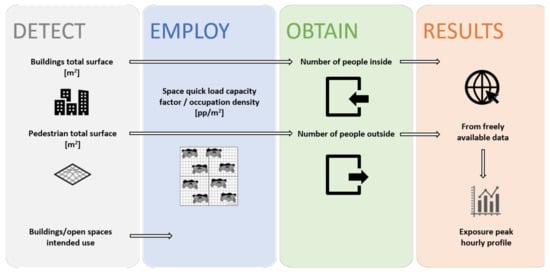
Figure 2.
General operational framework representation for peak exposure detection.
People exposed to SLODs were considered as those who were either inside or outside buildings. Given the nature of the SLODs, unfolding over months or even years, they act on people which are repeatedly exposed to unfavorable conditions; such as residents, frequent visitors, and/or workers of the commercial establishments in the area, who are constantly coming into and out of the studied area. Moreover, outdoor heat stress and air quality are directly affecting indoor temperature and air pollution. To quantify these number of people exposed, four main steps are identified and described as follows:
- Detect the buildings’ intended use in the studied area. Hence, where available, GIS tools could support and facilitate the labeling process. Then, in locations where such information is not present, tools like Google Maps application [30] offer maps where indications related to public facilities are freely available (e.g., offices, schools, hospitals, homeless centers, theatres). Additionally, this same tool offers for each public facility and commercial activities, further information; for example, its denomination, the address, and opening times. Furthermore, the Google Street view application [31] can be employed to detect punctually buildings that host more than one activity or different intended use; for example, economic activities placed at the ground level of inspected buildings, while upper levels host private dwellings. Hence, it can be assumed that the remaining built volume where no activities open to the public are observed constitutes the residential part of the BE. Further verifications can be performed by one-site surveying.
- Estimate the maximum admissible occupancy (in terms of the number of people) of indoor environments for all the previously detected buildings intended use. To reach this goal, national/regional/local occupancy density guidelines can be employed (e.g., housing, fire safety, energy modeling regulations) which prescribe for each intended use a direct load capacity factor (e.g., load capacity factor from the Italian fire safety regulations, see Table 1). Load capacity factors are commonly given in terms of the assumed number of people per square meter (pp/m2). Later, the total area of each intended use is calculated and multiplied for the corresponding factor to obtain the maximum admissible occupancy for a specific place (or determined area), which when reached can be assumed as a critical peak of exposure.
 Table 1. Simplified occupant load factors for different intended use are reported referred to Italian fire safety regulations.
 - From a practical point of view, the extension area for each building can be determined with a remote data collection approach. This is possible through the use of GIS tools, or thanks to tools such as “Map Area Calculator” on CalcMaps [32]. The latter requires delineating the planar covered area of the studied element (e.g., buildings covered area) visualized on the map which returns an estimated area cover. Building floors are then counted individually through Street View visualization. The planar covered area is multiplied for the evinced number of floors related to a specific building function, in such a way, each intended use extension is sized.
- Estimation of the study area inhabitants. To do so, population census data can be used to quantify the population by using municipal scale data as representative of the number of exposed people within the case study. Census data provides sufficient demographic information, including a diversification by different age ranges and occupations. However, inhabitants cannot be considered inside their dwelling for all day; that is, certain age ranges are expected to be working (i.e., working-age group) and attending education facilities outside the studied area. Therefore, making use of statistically constructed building occupancy profiles, such as the ones used for building energy performance computation [33], it is possible to obtain the schedules in which most likely workers and students are expected to be outside. Hence, the present methodology supposes the subdivision of hosted inhabitants and occupied schedules in the following way:
- toddlers and elders, or retired, residents spend most of their time at home or in their home surroundings (24 h presence);
- young people, in specific students, spend school hours (between 08:00 and 13:00) at schools, away from the studied area (unless it hosts education facilities) and the remaining time they are considered to stay at home; and,
- adults are expected to spend their working time away from home (between 08:00 and 18:00).
Seasonal and weekday/non-working day variations are not considered, including these would be out of the scope of this work. Each percentage of these three citizens’ typology is associated in proportion to the total number of the resident within the case study esteemed by multiply the residential surface for the related occupation density factor. - Similar consideration can be also traced for estimating the occupancy of the remaining functions of indoor spaces. However, a deeper focus based on the subdivision of people presence variance during the day can be done from additional online available data. For instance, Google Maps [30], provides additional information such as the working days and opening times. Following such data for each hour of the day, it is possible to include a more precise estimation of the actual number of occupants present for each of the non-residential functions reducing the potential overestimation of people considered within the analyzed BE.
- Additionally, the occupation of outdoor pedestrian areas (computed from the remaining area after subtracting, from the total area, the spaces occupied by buildings and carriageways) that casually move through the case study portion is assumed constant during the surveyed opening hours of the non-residential functions found within the area of study.
Nevertheless, the basic estimation of the number of occupants inside the intended uses according to the previous steps constitutes an unlikely condition as it is expressed as the maximum probable occupancy. Thus, after obtaining the maximum probable occupancy the daily exposure profile can be further adjusted with the adoption of an additional weighting factor for a more precise daily variation of citizens’ presence (as the ones given by ISO 17772 [33] for residential and popular times for commercial spaces).
2.3. Critera for Peaks Merging
After the multi-hazard risk arousal and exposure peaks have been constructed as daily profiles (having one value per hour), their superimposition is possible sharing the x-axis (i.e., Hour of the day [h]). This would permit a direct qualitative comparison of the temporal domain in which the multi-hazard existence is more likely, and the exposure has been proven high.
Moreover, if the collected data is sufficient, it will be possible to differentiate the degree of exposure by demographic groups, allowing to spot those at higher risk exposure to support decision-making on intervention plans and strategies. On the other hand, identifying the buildings of the studied zone which generate higher exposure (i.e., crowding sources), provides additional information on crowding sources to deploy targeted and efficient mitigation solutions.
On the other hand, for quantitative integration of hazard and exposure data, in order to obtain a simplified but unified degree of risk (R), the online multi-criteria decision method of Analytic Hierarchy Process (AHP) was utilized [46]. This allows to introduce of the individual vulnerability (V) based on the demographic groups present in the analyzed area, by splitting the exposure (E) into the present groups and providing each of them a weight (w) to this presence based on their susceptibility to such hazard (increasing temperatures (h) and air pollution (p)); see Equations (1) and (2). Then, these are multiplied by the weighted peak frequency of the respective hazard to obtain the degree of risk (R) for such SLOD type or its combination; see Equations (3)–(5).
where expe is meant to have the normalized exposure of elders; exptd is the normalized exposure of toddlers; expad: adults exposure; freqp is the hazard frequency probability for severe air pollution; freqh is the hazard frequency probability for severe heat stress; V&Ep is the Vulnerability and Exposure degree obtained for air pollution; V&Eh is the Vulnerability and Exposure degree obtained for heat stress; wp_e is the weight-related to air pollution vulnerability associated to elders; wp_td is the weight-related to air pollution vulnerability associated to toddlers; wp_ad is the weight-related to heat stress vulnerability associated to adults; wh_e is the weight-related to heat stress vulnerability associated to elders; wh_td is the weight-related to heat stress vulnerability associated to toddlers; wh_ad is the weight-related to heat stress vulnerability associated to adults; wp is the weight related to the criticality of air pollution hazard; wh is the weight related to the criticality of heat stress hazard.
V&Ep = wp_e × expe + wp_td × exptd + wp_ad × expad
V&Eh = wh_e × expe + wh_td × exptd + wh_ad × expad
Rp = freqp × V&Ep
Rh = freqh × V&Eh
Rmhz = wh × Rh + wp × Rp
Finally, for the estimation of the multi-hazard risk (Rmhz), the values obtained for increasing temperatures (Rh) and air pollution (Rp) are multiplied. These values are then plotted to unveil and understand which timeframe is associated with the highest risk for each demographic group in the analyzed area.
2.4. Case Study Presentation
Following the analysis done by Salvalai et al. [10], Milan (Italy) is a representative case study to assess the contemporaneous phenomena of increasing temperatures and air pollution hazards on a densely populated metropolis; and at a smaller scale, the geographical Local Identity Unit (NIL) of Città Studi.
Italy, and in particular the northern part of the country, has been labeled on the Emergency Events Database (EM-DAT) [47] as an “extreme temperature affected country” and the European Environment Agency (EEA) [6] has reported a 0.3–0.35 °C average annual temperature increase trend for the same area. In addition, for the matching region, the World Health Organization (WHO) [48] reported annual mean concentrations of particulate matter (i.e., PM2.5) that go beyond healthy limits, being worse for the city of Milan.
In this context, the SLODs risk in Milan is worsened by the population density it holds. Milan is within the most populated region in Italy (i.e., Lombardy). The city of Milan itself hosts approximately 3.5 million people [49].
From available datasets on the Municipality of Milan’s website [50], it was deduced by [10] that the Città Studi area is characterized by high population density with heterogeneous infrastructure and BE typologies. It was described as a rather distinct area, in which:
- An average concentration of susceptible population can be found (adults over 65 and toddlers below 5 years old represent 22.3%), in fact, two home cares are located near the boundary limits and more than 20 educational institutes are hosted.
- one reliable data source for monitoring air quality is within the boundary limits (Milano—Pascal Città Studi) and one more adjacent was found for supervising both air quality and weather fluctuations (Milano—via Juvara).
- It can be assumed as a low heat and pollutant management area given its low greenery area coverage (15.4%), fairly high built surface area (29.4%), and volume coverage.
A narrower area was delineated as a representative portion of the identified NIL (see Figure 3), to simplify the analysis and enable data collection and processing. This narrowed site hosts a significant number of residents; it contains different urban BE types with busy roads (such as piazza, Piazzale, and urban canyon), holds potential crowding points (two schools, one nearby university, a sports center, a theatre, and a religious building), has a nearby waterbody and embedded greenery.
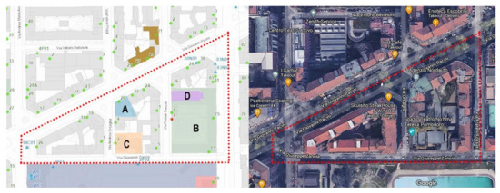
Figure 3.
Delineated case study area (dotted red line) with the identification of public facilities to compute exposure. A comparison is given between the results obtained through GIS tools (left side) and Google Maps (right side); Civic numbers in the GIS visualization are also provided in correspondence of the green points for both public buildings and private dwellings. The GIS map is available at Comune di Milano Geoportale [51] and was furtherly elaborated by the authors.
3. Results
3.1. SLOD Peaks Identification
These results are a more granular analysis of what has been already presented in Blanco Cadena et al. [26], by utilizing larger time-series datasets to better estimate the likelihood of synergic SLODs arousal during the day.
For the selected case study, data were extracted from the regional environmental monitoring institution ARPA Lombardy Agency [52], which shares openly its environmental monitoring measurement database, making it possible to retrieve air quality and weather data from Milano Pascal Città Studi and Milano v. Juvara stations (stations that are 600 m and 1.03 km, respectively, from the center of the narrowed site). These data were collected and elaborated for the 2015–2019 time period, prioritizing yearly data completeness and recentness.
Unfortunately, there was not a single station equipped with both air quality and weather sensors to gather data from. However, both enquired stations are relatively close from one to another, they are located within similar urban contexts, with low green area coverage and mid-high built density. Thus, data collected is expected to have similar trends and show sufficient evidence that this portion of the city has reduced heat and pollution management capacity.
3.1.1. Heat Stress Estimation
Data gathered from the weather station Milano v. Juvara was incomplete to compute the UTCI; that is, not sufficient information was surveyed to estimate mean radiant temperature. Therefore, the extent of the heat stress on citizens was computed for outdoors and walking pedestrians using RiskT [26] (employing only air temperature, solar radiation, wind speed, and relative humidity), assuming that they will be exposed to the effect of direct solar radiation and diminished air velocity (warmer sensation). The weighting factors were maintained as:
- tdb-air = 0.4 for temperatures above 26 °C;
- tdb-air = −0.4 for temperatures below 18 °C;
- Itot = 0.3 for irradiation over 300 W/m2;
- RH = 0.15 for values below 30% or above 70%; and
- Va = 0.15 for values below 2 m/s.
Using these settings, RiskT was computed summing the weights for every monitored hour from 1 January 2015 00:00 to 31 December 2019 23:00 (44124 h screened) to determine the existence of heat stress (heat risk = TRUE if RiskT > 0.5). From which, only 438 (<1%) were found to have at least one missing datum; thus, it was reasonable not to perform any data completion. A description of the weather dataset is presented in Table 2.
Table 2.
Studied weather dataset description summary.
Air temperature peaks were registered over a 5-year period at 38 °C, while global horizontal radiation reached 952 W/m2 as a maximum registered value. On RiskT, variance is high (std = 0.32) but there were times in which all the parameters were measured at an uncomfortable range. Categorizing RiskT, more than 5000 h were reported having a hazardous heat stress condition during the analysis period, which represents approximately 12% of the collected data.
Then, the discrete 0 (FALSE) and 1 (TRUE) values of heat risk were grouped and averaged by each of the 24 h of a single day to establish the frequency in which heat risk hazard arise (freqh). These showed peaks of frequency arousal between 10:00 and 18:00, with the maximum frequency probability during the 15:00 and 16:00 h. These probability values were summarized together with the ones obtained for air quality in Table 3.
Table 3.
Frequency probability profile data of heat (freqh), pollution (freqp), and multi-hazard risk (freqmhz) for those hours of the day considered with more human activity.
3.1.2. Determining Air Quality Condition
Air quality sensors were found scarcely diffuse within the city of Milan, likewise, their latency was limited. Sufficient data was only found for particulate matter (i.e., PM10, PM2.5), ammonia (NH3), and ozone (O3). Air quality was expressed as AQI, based on healthy exposure limit values for 8-h average and the 8 h moving average of air pollutant concentration. Finally, the air pollution distress (pollution risk = TRUE) was set to AQI > 100, which is the limited exposure of demographic groups that are sensitive to such substances (toddlers and elders) [28].
The AQI was also screened for the same analysis period; but, more than 13,000 h had at least one missing datum. Nevertheless, as done for heat stress no data completion process was performed given that: AQI is determined as the maximum value from the air pollutants concentration; for which O3 is the most representative, having the largest mean value (in consequence, largest mean AQI) and it is the one with the least missing values (approximately 2%). A detailed description of the weather dataset is presented in Table 4.
Table 4.
Studied air quality dataset description summary.
Similar to what was encountered on RiskT, the AQI variance is high (std = 40.53). Over a 5-year period, for Milan an average value of AQI near a risky threshold limit is serious (AQI = 87.08), and a maximum value that doubles the suggested minimum 8-h exposure is severe. Moreover, the fact that more than 33% (14,576 h) of the time citizens, if present, were exposed to poor air quality demands urgent mitigation measures.
Then, as reported in Table 3, the hourly frequency probability of pollution hazard risk (freqp) in a typical day was computed, resulting in a high likelihood of arousal from 15:00 onwards and a maximum peak of such likelihood at 19:00 h. In fact, sufficient evidence was collected to assume that in this area polluted air at night hours was common for the selected analyzed period.
3.1.3. Synergic Heat and Air Pollution Distress
As the high likelihood of critical hazard arousal was found to coincide, it was relevant to identify the frequency with which both hazards are present simultaneously, as this timeframe would be crucial for whoever is both vulnerable and exposed.
Heating risk and pollution risk condition Boolean were multiplied to obtain only those cases in which both risks were synergic. Hence, within the selected analysis period, more than 2000 h (4.91%) were found to be under the synergic critical effect of heat and air pollution. These hazardous events were found to coincide more frequently (freqmhz) at 16:00, but with a high likelihood (>0.09) of arousal between 14:00 and 18:00.
The above is clearly visible in Figure 4, where the frequency of poor air quality (AQ) conditions is higher in the early and late hours of the day; while the heat stress conditions are more marked slightly after midday. Nevertheless, their aggregated effect and risk (Agg. risk) is significant in the afternoon.
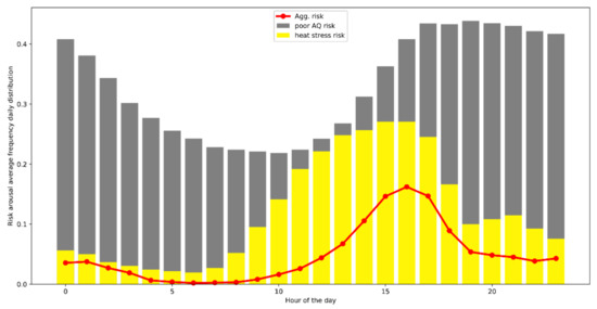
Figure 4.
SLODs risk hazard frequency probability profile superposition. Differentiating between air pollution distress (poor AQ risk), heat stress, and their aggregated hazard risk (Agg. risk) arousal frequency.
3.2. Exposure Peaks Identification
The methodological framework presented in Section 2.2 is applied to the specific case study presented in Section 2.4. Firstly, the buildings intended uses are evaluated mainly through Google Maps and the Street View tools. A further verification about the reliability of collected data from online tools was also performed thanks to the availability of the Milan Municipality of an open-source GIS portal. Figure 3 shows within the study area the presence of four main public activities: a homecare center for young mothers, a school with different grades of instruction, a theatre with 250 seats, and finally the church of Santa Maria Assunta. Additionally, only through the employment of such tools was it possible to determine the presence of additional small commercial activities at the ground level of several buildings, not documented in the GIS database. Especially, commercial places were detected such as local shops, restaurants, bars, and other specific activities which could attract citizens such as a bank, a travel agency, and private professional studies (e.g., doctors and dentists). The remaining buildings (that in the GIS visualization from Figure 3 are grey) constitute the private dwellings each one identified by their own civic number; while in Google Maps such private function is not punctually specified, it can be indirectly deduced by screening the are throughout Street View.
Then, the required geometrical features of buildings were surveyed in order to determine the maximum crowd conditions (i.e., floor areas). Table 5 associates each building with its number of floors, their planar area extension, the total usable area, their corresponding load capacity factor, and the total estimation of people present in the number of people (pp).
Table 5.
Buildings geometrical and occupancy features: the total area covered by each building’s intended use; their occupancy load capacity factor; and, the maximum occupancy capacity (maximum number of people [pp]), esteemed by multiplying maximum load capacity factor (pp/m2) and the total area of each building.
Starting from the evaluation of the total number of people that can be simultaneously present in the case study area, additional assumptions lead to estimate a reduced number of people in a specific hour of the day in order to reach a more representative and realistic scenario of the ordinary conditions; for instance, the analysis was carried out only for working days, so to consider people leaving for work and visitors coming into non-residential functions. The total maximum number of people of the delineated area is easily obtained by summing the partial estimates for each building of Table 5; only for residential intended use, the maximum number of inhabitants is estimated at 1380. Further information about the hosted inhabitants demographics in the case study area were retrieved from census data according to Section 2.2. From such data, proportions for age-related group ranges for the Milan Municipality (representative of the case study urban tissue) are utilized.
Italy considers 15 to 64-year-old citizens as falling into the working age group and, in Milan during 2020, more than 60% of youngsters (15–24-year-old range) were still studying [53]; thus, <5 years old were considered as toddlers, 5–24 years old inhabitants were considered as students, 25 to 64 were considered workers and >65 were considered as elders. Results show a population composed of 22.3% of toddlers and elders, 60.3% of adult workers, and 17.4% by students. Hence, it would be reasonable to assume that from 1380 inhabitants, 308 are toddlers and elders, 832 adult workers, and 240 students who live in this delineated BE portion. Withal, an hourly profile in terms of the number of residents was defined considering the previously established schedules per resident type; see Table 6.
Table 6.
Results related to the individuals’ presence in the studied area (exposure peak) is offered hour by hour highlighting only the “Residents” component, the “visitors” component, by summing each component with the number of people along the streets in “Total”, and a “Ratio” computed by normalizing each value by the maximum obtained “Total” occupancy.
Successively, the same hourly profile was traced for non-residents (e.g., visitors) that comprehend all the individuals that could potentially populate the studied area for working, studying, and/or enjoying the facilities, private shops, and restaurants (see Table 4). Thanks to the collected opening and popular times of all these commercial establishments, the occupancy profile can be discretized and weighted by the hour.
The exposure peaks estimated so far concern only the total sum of residents and non-residents indoors (“Total” in Table 6); thus, the number of pedestrians passing through the open spaces of the studied area for each hour is missing. Then, pedestrians along the streets are assumed constant at 38 ppl (given the pedestrian lanes’ area extension) during the time that commercial establishments were found to be open during the day (from 7 a.m. to 12 p.m.). All these results allow us to delineate the hourly profile of working days of exposure for the Milan case study graphically visualized in Figure 5.
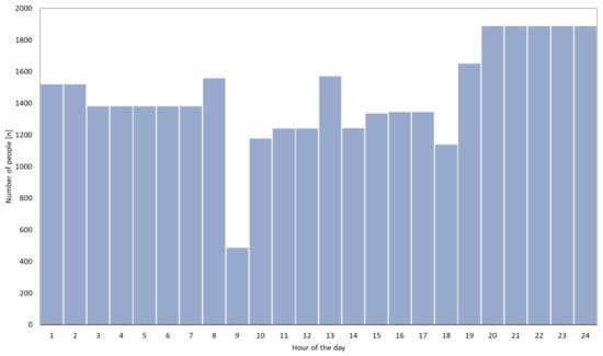
Figure 5.
Exposure peak hourly profile including the occupation dynamics of the considered demographic groups (i.e., elders, adult workers, students, and toddlers).
The obtained profile in Figure 6 is characterized by a high number of people present early in the morning and at night. This represents people at and returning to their own dwellings and the visitors that would populate restaurants and bars still open in the area. Such exposure peaks are clearly related to the hosted function of buildings in the studied spaces. However, a high concentration of people in public buildings and social functions is exhibited, frequenting near economic activities such as shops or bars, and restaurants. Although the exposure peak is lower than the previously described situation, also in such conditions, increasing values of people are registered during morning hours especially in the second part of the morning (e.g., 10 a.m. to 1 p.m.); or, when the students are back from school and non-residential functions begin to open (i.e., from 15:00 to 17:00).
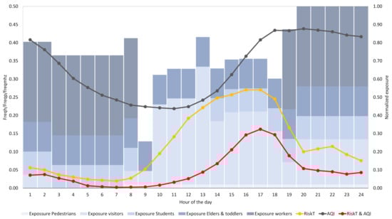
Figure 6.
Qualitative superposition of exposure peaks and hazard frequency probability of arousal.
3.3. Input Scenarios for Simulation
The input scenarios for studying the human behavior analysis, in specific, their interaction with the environment and the BE shall be selected based on the risk level found for such input scenarios. From a rapid qualitative assessment on Figure 6, and considering the assumptions of residents behavior dynamics (i.e., occupation profiles), one can note how late on the evening and early in the morning residents of such delineated region are at a high risk of air pollution SLOD; while late in the afternoon, students and regular visitors would be more at risk of suffering from increasing temperatures SLOD, and from a conjoint effect of both.
Moreover, the AHP methodology is applied to introduce vulnerability together with exposure to enable an estimate of the risk an inhabitant of the delineated area would be subjected to. To do so, the susceptibility of the studied demographic groups were established based on their mortality risk increase when exposed to extreme heat events and high air pollution conditions compare to a control group. However, as there is no information on how diverse pedestrians and visitors are they were weighted equally to the adults to avoid additional overestimation of the risk. Sufficient evidence has shown that elders and toddlers are similarly susceptible when subjected to such conditions. In fact, elders have been reportedly found to be 1.24 and 1.20 more susceptible than healthy adults to heatstroke and respiratory disease respectively [54,55]. Hence, using the online tool offered by Goepel [46] it was possible to obtain:
- wp_e = wp_td = 0.75
- wh_e = wh_td = 0.75
- wp_ad = 0.25
- wh_ad = 0.25
Then, comparing the Emergency Events Database (EM-DAT) [47] on heatwave deceases for the previous years and the corresponding number for attributed or related deceases to air pollution in Europe [56], it was found that they are on an approximate 1:10 ratio. Thus, the following weights were allocated to compute the overall multi-hazard analysis employing Equations (3) and (4).
- wp = 0.9
- wh = 0.1
Finally, it was possible to lay down a daily risk profile for each SLOD type and one regarding their conjoint effect. These are compared in Figure 7.
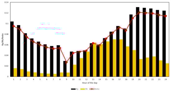
Figure 7.
Estimation of SLODs risk daily profiles. Comparison between heat-related (Rh), air pollution-related (Rp), and multi-hazard risk (Rmhz).
Given the severe impact of air pollution, most of Rmhz trend is driven by the trend of SLOD air pollution. Nevertheless, just after midday, the heat-related risk (Rh) is as significant as the one reported for air pollution. It is noteworthy that the highest risk value is reported for late hours during the day, in which most residents would be present in the studied area.
Therefore, analyzing both Figure 6 and Figure 7 for the analyzed area, relevant input scenarios for people behavior and BE interaction modeling considering environmental stressors any of the environmental and exposure conditions of the period between 13:00 and 17:00 would be good for considering both heat and polluted air including diverse demographics. Another relevant input scenario could be the study of night hours, although most of the residents are meant to be resting and the visitors are significantly reduced.
4. Discussion
A flexible and easily applicable procedure for assessing the daily fluctuation of each SLOD and the combination of critical SLODs risk has been proposed; and, its applicability has been tested for studying the SLODs risk condition of a specific, but relevant, case study in the City of Milan, Italy.
The work allowed to adjust and refine the steps presented for the methodology, identifying possible gaps or challenges that researchers and designers must face when assessing the BE actual and future conditions (analyses can be done as well with future, forecasted, climatic data).
For the specific case study, the procedure allows for unveiling how severe the risk is at which residents of such neighborhood have been and would probably be subjected to in the future. In particular, the overall risk and the air pollution risk are stronger at night (Rp > Rmhz > 0.1). This can generate healthy affections and others. Meanwhile, visitors and students are more prone to suffer the effects of both heat-related and air pollution SLOD affections by midday.
The fact that the impact of air pollution was established as dominant (i.e., 1 to 9 ratio), undermines the significant burden caused by increasing temperatures, especially with the previously mentioned air temperature trends, this is likely to change.
The methodology presents itself as relevant for any type of human behavior analysis, and in particular its interactions with the BE. It does provide information on what type of environmental stressors to include, as well as, sufficient data on the number of people the simulation should consider (e.g., agents), the demographic groups to employ, and the time in which these simulations should be performed.
Methodology Limitations and Further Work
The methodology has been laid down to enable a multi-hazard SLOD risk analysis with limited information and utilizing open-source tools. However, in certain locations available data could be even more restrained resulting in higher variance:
- no environmental data in the surrounding studied area;
- no specific data on the features of the BE without the possibility of on-site survey (or impractical due to area extension); and,
- no demographic information of the site.
For the methodology used to estimate hazards, two locations were used for collecting data (i.e., Milano v. Juvara and Milano Pascal Città Studi) which might differ from the actual site micro-climatic conditions. RiskT, and not UTCI, heat stress indicator was used, which accounts for the indirect effect of the BE features on the augmented heat perception of the actual position a person can be located.
Meanwhile, in relation to the methodology proposed for estimating exposure, and in particular for the presented case study, the use of load capacity factors overestimates the potential real number of people present in the studied area. The presence of visitors in non-residential functions can be further refined by collecting data on the relative value of occupation given by the location’s popular times. Or, if sufficient data is available from census data, more precise values can be used to compute the real number of people exposed to the hazard; presenting the values as a relative/normalized proportion, reduces this uncertainty.
For the holistic risk estimation, and the peaks merging, a more detailed study is foreseen to properly identify the vulnerability weighting factors specifically for toddlers and students with respect to the adults. This is planned to be refined by digging deeper in the literature about the differences in the homeostatic capacity of the human body and its differences in age, this was not considered as it exceeds the scope of the present work.
Nevertheless, the proposed methodology represents a useful tool to be used when there is scarce information available of the studied area. It does not require complex computation techniques or machines to rapidly estimate the risk hourly.
Being able to define critical hazard-exposure scenarios from input data, the proposed methodology could analyze potential future risk conditions, or compare actual with previously experienced circumstances, by manipulating the information used for the analysis. That is, modifying input climate data (surveyed climate or forecasted climate change scenarios) and demographic data (past, actual, or future trends on occupancy and/or demographics). In addition, the proposed framework would be also capable of defining risk scenarios under extraordinary social conditions, or measures (e.g., lockdowns and curfews), that affect the occupancy trends by adjusting accordingly the weights of the space occupancy profiles.
5. Conclusions
Urban BEs are increasingly prone to SLODs, such as air pollution and heatwaves. The effectiveness of risk-mitigation solutions should be defined and tested by considering critical scenarios. Combining environmental conditions, exposed users’ presence, and vulnerability, and behaviors is a paramount task to support decision-makers in risk assessment.
Evidence has shown how people living in the BE are highly at risk of SLODs, and especially within highly urbanized areas that have reduced green area coverage and intense pollutants emission/concentration. It is a fact that in the last decade hospital admissions and deceases, related to reduced air quality and/or increased air temperatures, have raised [54,55]. Hence, designers that influence the BE should analyze the current BE features and the evolution of the environmental conditions to enact effective mitigation strategies.
The current methodology identifies hazard frequency probability, exposure levels, and the extent of vulnerability based on available data of demographic groups and literature findings. In addition, it provides suggestions on which type of data to access and which tools to use to gather it (even in the case of absence).
For instance, for the case study in which the methodology has been applied, it was possible to individuate single-hazard and multi-hazard risk for a representative portion of the city. Exposure was computed from functional occupation density and the extent of the function’s physical space. Vulnerability was introduced by means of weights based on the fragility of certain demographic groups, and hazard was provided by estimating the frequency of the existence of critical conditions. As an outcome, it was possible to communicate that residents are constantly exposed at night to hazardous air pollution concentrations even when indoor; meanwhile young adults, visitors, and elders are exposed to both critical heat stress conditions during the day and unhealthy air quality at night.
The applicability and robustness of the framework have also been proven by being flexible with the type of heat stress or air quality criteria; the ease of data collection for exposure, vulnerability, and hazard; and also, the possibility of utilizing different input data for comparing past, present and predicted conditions (e.g., climate change, demographic change, social trends).
Author Contributions
Conceptualization, J.D.B.C., M.L., G.S. and E.Q.; methodology, J.D.B.C., G.S. and M.L.; validation, J.D.B.C., G.S. and E.Q.; formal analysis, J.D.B.C., M.L.; investigation, J.D.B.C. and M.L.; resources, G.S. and E.Q.; data curation, J.D.B.C. and M.L.; writing—original draft preparation, J.D.B.C. and M.L.; writing—review and editing, J.D.B.C., G.S., E.Q. and M.D.; visualization, J.D.B.C. and M.L.; supervision, G.S. and E.Q.; project administration, G.S. and E.Q.; funding acquisition, G.S. and E.Q. All authors have read and agreed to the published version of the manuscript.
Funding
This research was funded by the MIUR (the Italian Ministry of Education, University, and Research) Project BE S2ECURe—(make) Built Environment Safer in Slow and Emergency Conditions through behavioUral assessed/designed Resilient solutions (Grant number: 2017LR75XK).
Institutional Review Board Statement
Not applicable.
Informed Consent Statement
Not applicable.
Data Availability Statement
Publicly available datasets were analyzed in this study. Utilized ata can be found in the following links: https://www.arpalombardia.it/Pages/Temi-Ambientali.aspx (accessed on 4 November 2020); http://dati.istat.it/ (accessed on 4 November 2020); http://dati.comune.milano.it/ (accessed on 4 November 2020); and, https://geoportale.comune.milano.it/ (accessed on 4 November 2020).
Conflicts of Interest
The authors declare no conflict of interest.
References
- Siegele, L. Loss and Damage: The Theme of Slow Onset Impact; Germanwatch: Berlin, Germany, 2012; Volume 1, pp. 1–20. [Google Scholar]
- Salvalai, G.; Moretti, N.; Blanco Cadena, J.D.; Quagliarini, E. Slow Onset Disaster Events Factors in Italian Built Environment Archetypes. In Sustainability in Energy and Buildings 2020; Littlewood, J., Ed.; Springer: Singapore, 2021; pp. 333–343. [Google Scholar]
- Robinson, P.J. On the Definition of a Heat Wave. J. Appl. Meteorol. 2001, 40, 762–775. [Google Scholar] [CrossRef]
- Meehl, G.A. More Intense, More Frequent, and Longer Lasting Heat Waves in the 21st Century. Science 2004, 305, 994–997. [Google Scholar] [CrossRef] [PubMed]
- Guerreiro, C.B.B.; Foltescu, V.; de Leeuw, F. Air quality status and trends in Europe. Atmos. Environ. 2014, 98, 376–384. [Google Scholar] [CrossRef]
- EEA. Observed Annual Mean Temperature Change from 1960 to 2019 (Left Panel) and Projected 21st Century Change Under Different Emissions Scenarios (Right Panels) in Europe. Available online: https://www.eea.europa.eu/data-and-maps/figures/trends-in-annual-temperature-across-1 (accessed on 31 March 2020).
- Jamei, E.; Rajagopalan, P.; Seyedmahmoudian, M.; Jamei, Y. Review on the impact of urban geometry and pedestrian level greening on outdoor thermal comfort. Renew. Sustain. Energy Rev. 2016, 54, 1002–1017. [Google Scholar] [CrossRef]
- Kumar, P.; Abhijith, K.V.; Barwise, Y. Implementing Green Infrastructure for Air Pollution Abatement: General Recommendations for Management and Plant Species Selection; University of Surrey: Guildford, UK, 2019. [Google Scholar] [CrossRef]
- Barwise, Y.; Kumar, P. Designing vegetation barriers for urban air pollution abatement: A practical review for appropriate plant species selection. NPJ Clim. Atmos. Sci. 2020, 3, 1–19. [Google Scholar] [CrossRef]
- Salvalai, G.; Enrico, Q.; Blanco Cadena, J.D. Built environment and human behavior boosting Slow-onset disaster risk. In Proceedings of the Heritage 2020, Coimbra, Portugal, 8–10 July 2020; pp. 199–209. [Google Scholar]
- Yıldız, B.; Çağdaş, G. Fuzzy logic in agent-based modeling of user movement in urban space: Definition and application to a case study of a square. Build. Environ. 2020, 169. [Google Scholar] [CrossRef]
- Melnikov, V.R.; Krzhizhanovskaya, V.V.; Lees, M.H.; Sloot, P.M.A. The impact of pace of life on pedestrian heat stress: A computational modelling approach. Environ. Res. 2020, 186, 109397. [Google Scholar] [CrossRef] [PubMed]
- Liang, S.; Leng, H.; Yuan, Q.; Wang, B.W.; Yuan, C. How does weather and climate affect pedestrian walking speed during cool and cold seasons in severely cold areas? Build. Environ. 2020, 175, 106811. [Google Scholar] [CrossRef]
- Yang, L.; Hoffmann, P.; Scheffran, J.; Rühe, S.; Fischereit, J.; Gasser, I. An Agent-Based Modeling Framework for Simulating Human Exposure to Environmental Stresses in Urban Areas. Urban Sci. 2018, 2, 36. [Google Scholar] [CrossRef]
- Briggs, D.J.; de Hoogh, K.; Morris, C.; Gulliver, J. Effects of travel mode on exposures to particulate air pollution. Environ. Int. 2008, 34, 12–22. [Google Scholar] [CrossRef]
- Amorim, J.H.; Valente, J.; Cascão, P.; Rodrigues, V.; Pimentel, C.; Miranda, A.I.; Borrego, C. Pedestrian exposure to air pollution in cities: Modeling the effect of roadside trees. Adv. Meteorol. 2013, 2013. [Google Scholar] [CrossRef]
- Borrego, C.; Valente, J.; Amorim, J.H.; Rodrigues, V.; Cascão, P.; Miranda, A.I. Modelling of tree-induced effects on pedestrian exposure to road traffic pollution. WIT Trans. Built Environ. 2012, 128, 3–13. [Google Scholar] [CrossRef]
- Bisson, M. Simulazione del microclima urbano di Milano mediante il software ENVI-met. In Studio degli Effetti dell’Inserimento di Aree Verdi sulla Sollecitazione Termica degli Edifici; Politecnico di Milano: Milan, Italy, 2010. [Google Scholar]
- De León, J.C.V. Vulnerability: A Conceptual and Methodological Review; UNU Institute for Environment and Human Security: Bornheim, Germany, 2006. [Google Scholar]
- D׳Orazio, M.; Quagliarini, E.; Bernardini, G.; Spalazzi, L.; D’Orazio, M.; Quagliarini, E.; Bernardini, G.; Spalazzi, L. EPES–Earthquake pedestrians’ evacuation simulator: A tool for predicting earthquake pedestrians׳ evacuation in urban outdoor scenarios. Int. J. Disaster Risk Reduct. 2014, 10, 153–177. [Google Scholar] [CrossRef]
- Delfino, R.J.; Tjoa, T.; Gillen, D.L.; Staimer, N.; Polidori, A.; Arhami, M.; Jamner, L.; Sioutas, C.; Longhurst, J. Traffic-related air pollution and blood pressure in elderly subjects with coronary artery disease. Epidemiology 2010, 21, 396–404. [Google Scholar] [CrossRef]
- Barrow, M.W.; Clark, K.A. Heat-related illnesses. Am. Fam. Physician 1998, 58, 749. [Google Scholar]
- Koks, E.E.; Jongman, B.; Husby, T.G.; Botzen, W.J.W. Combining hazard, exposure and social vulnerability to provide lessons for flood risk management. Environ. Sci. Policy 2015, 47, 42–52. [Google Scholar] [CrossRef]
- Capgemini Institute; European Commission. Creating Value through Open Data: Study on the Impact of Re-Use of Public Data Resources; European Union: Luxembourg, 2015; ISBN 9789279527913. [Google Scholar]
- Happle, G.; Fonseca, J.A.; Schlueter, A. Context-specific urban occupancy modeling using location-based services data. Build. Environ. 2020, 175, 106803. [Google Scholar] [CrossRef]
- Blanco Cadena, J.D.; Moretti, N.; Salvalai, G.; Quagliarini, E.; Re Cecconi, F.; Poli, T. A New Approach to Assess the Built Environment Risk under the Conjunct Effect of Critical Slow Onset Disasters: A Case Study in Milan, Italy. Appl. Sci. 2021, 11, 1186. [Google Scholar] [CrossRef]
- Calculating UTCI Equivalent Temperature. Available online: http://www.utci.org/utci_poster.pdf (accessed on 4 November 2020).
- U.S. Environmental Protection Agency. Guidelines for the Reporting of Daily Air Quality–The Air Quality Index (AQI); Office of Air Quality Planning and Standards: Triangle Park, NC, USA, 2006.
- MeshkinKiya, M.; Paolini, R. Preparing Weather Data for Real-Time Building Energy Simulation. arXiv 2020, arXiv:2011.09733. [Google Scholar]
- Google. Google Maps. Available online: https://www.google.it/maps?hl=en (accessed on 4 November 2020).
- Google. Google Street View. Available online: https://www.google.it/streetview/ (accessed on 4 November 2020).
- CalcMaps. Map Area Calculator. Available online: https://www.calcmaps.com/it/map-area/ (accessed on 26 January 2021).
- ISO. Energy Performance of Buildings—Indoor Environmental Quality—Part 1: Indoor Environmental Input Parameters for the Design and Assessment of Energy Performance of Buildings; ISO: Geneva, Switzerland, 2017. [Google Scholar]
- Dipartimento dei Vigili del Fuoco. Approvazione di Norme Tecniche di Prevenzione Incendi; Ministero dell’Interno: Rome, Italy, 2015.
- Dipartimento dei Vigili del Fuoco. Criteri Generali di Sicurezza Antincendio e Per la Gestione Dell’emergenza Nei Luoghi di Lavoro; Ministero dell’Interno: Rome, Italy, 1998.
- Dipartimento dei Vigili del Fuoco. Regolamento Contenente Norme di Sicurezza Antincendio per gli Edifici Storici e Artistici Destinati a Musei, Gallerie, Esposizioni e Mostre; Ministero dell’Interno: Rome, Italy, 1992.
- Dipartimento dei Vigili del Fuoco. Regolamento Concernente Norme di Sicurezza Antincendio per gli Edifici di Interesse Storico-Artistico Destinati a Biblioteche ed Archivi; Ministero dell’Interno: Rome, Italy, 1995.
- Dipartimento dei Vigili del Fuoco. Approvazione della Regola Tecnica di Prevenzione Incendi per la Progettazione, Costruzione ed Esercizio dei Locali di Intrattenimento e di Pubblico Spettacolo; Ministero dell’Interno: Rome, Italy, 1996.
- Dipartimento dei Vigili del Fuoco. Modifiche ed Integrazioni al Decreto del Ministro dell’Interno 19 Agosto 1996 Relativamente agli Spettacoli e Trattenimenti a Carattere Occasionale Svolti all’Interno di Impianti Sportivi, Nonche’ all’Affollamento delle Sale da Ballo e Discoteche; Ministero dell’Interno: Rome, Italy, 2001.
- Dipartimento dei Vigili del Fuoco. Modifica al Decreto 19 Agosto 1996, Concernente l’Approvazione della Regola Tecnica di Prevenzione Incendi per la Progettazione, Costruzione ed Esercizio dei Locali di Intrattenimento e di Pubblico Spettacolo; Ministero dell’Interno: Rome, Italy, 2012.
- Dipartimento dei Vigili del Fuoco. Norme di Prevenzione Incendi Per l’Edilizia Scolastica; Ministero dell’Interno: Rome, Italy, 1992.
- Dipartimento dei Vigili del Fuoco. Modalita’ di Trasmissione dei Bilanci e dei Dati Contabili degli Enti Territoriali e dei Loro Organismi ed Enti Strumentali alla Banca Dati delle Pubbliche Amministrazioni; Ministero dell’Interno: Rome, Italy, 2016.
- Dipartimento dei Vigili del Fuoco. Norme di Sicurezza per la Costruzione e l’Esercizio degli Impianti Sportivi; Ministero dell’Interno: Rome, Italy, 1996.
- Dipartimento dei Vigili del Fuoco. Modifiche ed Integrazioni al Decreto Ministeriale 18 Marzo 1996, Recante Norme di Sicurezza per la Costruzione e l’Esercizio degli Impianti Sportivi; Ministero dell’Interno: Rome, Italy, 2005.
- Dipartimento dei Vigili del Fuoco. Approvazione della Regola Tecnica di Prevenzione Incendi per la Progettazione, Costruzione ed Esercizio delle Attivita’ Commerciali con Superficie Superiore a 400 mq; Ministero dell’Interno: Rome, Italy, 2010.
- Goepel, K.D. Implementation of an Online Software Tool for the Analytic Hierarchy Process (AHP-OS). Int. J. Anal. Hierarchy Process 2018, 10. [Google Scholar] [CrossRef]
- D. Guha-Sapir EM-DAT, CRED/UCLouvain, Brussels, Belgium. Available online: www.emdat.be (accessed on 15 November 2020).
- World Health Organization. Monitoring Health for the SDGs; WHO: Geneva, Switzerland, 2019. [Google Scholar]
- ISTAT Statistiche Istat. Available online: http://dati.istat.it/ (accessed on 16 January 2020).
- Comune di Milano Portale Open Data|Comune di Milano. Available online: http://dati.comune.milano.it/ (accessed on 16 January 2020).
- Comune di Milano Geoportale. Available online: https://geoportale.comune.milano.it/MapViewerApplication/Map/App?config=%2FMapViewerApplication%2FMap%2FConfig4App%2F477&id=ags (accessed on 2 December 2020).
- ARPA Lombardia Dati e Indicatori. Available online: https://www.arpalombardia.it/Pages/Ricerca-Dati-ed-Indicatori.aspx# (accessed on 25 March 2020).
- Fioni, A.; Signorelli, A.; Cesare, V.; Verona, A.; Vaia, R.; Sgambetterra, V. Il Lavoro a Milano; CGIL: Milan, Italy, 2020. [Google Scholar]
- Wang, X.Y.; Barnett, A.G.; Yu, W.; FitzGerald, G.; Tippett, V.; Aitken, P.; Neville, G.; McRae, D.; Verrall, K.; Tong, S. The impact of heatwaves on mortality and emergency hospital admissions from non-external causes in Brisbane, Australia. Occup. Environ. Med. 2012, 69, 163–169. [Google Scholar] [CrossRef] [PubMed]
- Sharma, G.; Goodwin, J. Effect of aging on respiratory system physiology and immunology. Clin. Interv. Aging 2006, 1, 253–260. [Google Scholar] [CrossRef] [PubMed]
- EEA. Air Quality in Europe—2020 Report; Publications Office of the European Union: Luxembourg, 2020; ISBN 978-92-9480-292-7. [Google Scholar]


Publisher’s Note: MDPI stays neutral with regard to jurisdictional claims in published maps and institutional affiliations. |
© 2021 by the authors. Licensee MDPI, Basel, Switzerland. This article is an open access article distributed under the terms and conditions of the Creative Commons Attribution (CC BY) license (https://creativecommons.org/licenses/by/4.0/).