Evaluation and Influencing Factors of Industrial Pollution in Jilin Restricted Development Zone: A Spatial Econometric Analysis

Abstract

Winning the battle against pollution and strengthening ecological protection in all respects are vital for promoting green development and building a moderately prosperous ecological civilization in China. Using the entropy weight method, this paper establishes and evaluates a comprehensive industrial pollution index that contains and synthesizes six major industrial pollutants (wastewater, COD, waste gas, SO₂, NO_x, and solid waste) in the 2006–2015 period. Subsequently, this paper studies the spatiotemporal characteristics and influencing factors of industrial pollution via the Moran index and spatial econometric analysis. The empirical results indicate that (1) the temporal evolution of the industrial pollution index is characterized by an overall trend of first decreasing and then increasing. (2) The industrial pollution index of each county has certain geographical disparities and significant spatially polarized characteristics in 2006, 2009, 2012, and 2015. (3) The Moran test shows that there is a relatively significant spatial autocorrelation of the industrial pollution index among counties and that the geographical distribution of the industrial pollution index tends to show clustering. (4) Spatial regression models that incorporate spatial factors better explain the influencing factors of industrial pollution. The economic development level, technological progress, and industrialization are negatively correlated with industrial pollution, while population density and industrial production capacity are positively correlated. (5) Consequently, as relevant policy recommendations, this paper proposes that environmental cooperation linkage mechanisms, environmental protection credit systems, and green technology innovation systems should be established in different geographical locations to achieve the goals of green county construction and sustainable development.

1. Introduction

Over recent decades, the reform and opening up have produced remarkable contributions to economic growth that have achieved an unprecedented extraordinary leap from primary industrialization to industrial modernization at a large scale and at a rapid rate. However, the issue of environmental quality deterioration has become pressing and has inevitably resulted in a series of deep-seated contradictions and problems, arousing great concern from academics, government departments, and the general public [1]. The growing problem of environmental pollution is evolving into a bottleneck that is hindering China’s economic and social development. Simultaneously, industrial pollution stands out as one of the most crucial issues due to rapid industrial activities. Statistics show that industrial pollution accounts for approximately 70% of total environmental pollution, and the industrial production sector has become one of the major causes of environmental deterioration in the process of economic production. Industrial pollution triggers a series of remarkable negative impacts that not only adversely restrict sustainable development but also impose considerable pressure on ecological and environmental quality, which further poses an increasing threat to environmental security and public health [2,3]. To address environmental degradation and eliminate its negative effects, the Chinese government has made strenuous efforts to achieve a sustainable future by proposing an array of aggressive reduction policies, such as industry access lists, the closure of highly polluting factories, and environmental regulations. China has also officially provided enormous financial support for controlling industrial pollution. For instance, in 2015, a total of 77.368 billion yuan was invested to curb the increase in industrial pollution, constituting a growth rate of approximately 60% compared to the 2006 investment level of 48.395 billion yuan according to the statistics in the China Environmental Statistics Yearbook. Moreover, the Chinese government has formulated and launched pollution control targets based on which major environmental pollutants will be greatly reduced and the quality of the ecological environment will be improved as a whole in 2020 and be improved thoroughly in 2035. Currently, however, the reduction effects are not as positive as intended, and industrial pollution remains to be resolutely controlled to win the tough battle of pollution prevention in China. Therefore, a comprehensive and systematic investigation of the spatiotemporal characteristics and influencing factors of industrial pollution is essential to take effective environmental protection measures.

A restricted development zone is one of the key types of zones among the national major function-oriented zones, and restricted development zones are effective in optimizing the spatial pattern of national land space caused by the industrial layout and disorderly development [4,5]. Based on the orientations of development, large-scale, high-intensity industrialization, and urbanization are restricted to maintain and improve the supply capacity of agricultural products and ecological products. Restricting development inside a restricted development zone does not mean that economic growth is restricted or prohibited to protect the ecological security and food security in a region; rather, such restriction emphasizes the development degree of industrial activities and urbanization activities so that the ecological red line and resource supply are not compromised. In general, restricted development zones are areas with a weak resource carrying capacity and fragile ecological environmental systems. Furthermore, in such zones, ecological environmental protection policies must be implemented, and industrial development and the industrial layout must be strictly restricted to prevent effects on the ecological environment. From the perspective of the new regionalism, accumulating regional wealth is key to cultivating regional competitive advantages and enhancing regional sustainable development capabilities. Restricted development zones are economically underdeveloped areas that are facing huge economic development pressure. However, this type has a fragile ecological environment and a prominent contradiction between man and land. Various scholars focus on developed hot spot areas, such as megacities, major cities, and provincial capital cities in China, while scholars seldom pay attention to the former underdevelopment regions. This paper studies the state of industrial pollution of restricted development zone, which will help enrich relevant research content. The implementation of restricted development zones policy can affect the transformation of the regional economic development model to a certain extent, thereby affecting industrial pollution. Besides, it can optimize the spatial pattern of the country, force economic transformation and development, and promote the effective decoupling of pollution and the economy. We choose the restricted development zone as our research area, which is more typical and specific than other types of zones. Accordingly, studying the characteristics of the spatiotemporal evolution and confirming the influencing factors of industrial pollution hold great practical significance for preventing and managing environmental pollution risks in the context of the construction of the restricted development zone of Jilin Province (JRDZ).

The remainder of this paper is composed of five sections. Section 2 briefly reviews the relevant literature on industrial pollution. Section 3 introduces the study area, methodology and variables. Section 4 examines the empirical calculation results of the industrial pollution index and interprets the driving mechanism of industrial pollution. Section 5 draws relevant conclusions and proposes corresponding policy suggestions.

2. Literature Review

Numerous studies in the disciplines of geography and economics have extensively explored different industrial pollution emissions from different perspectives. Mainstream research on industrial pollution emissions mainly focuses on the status of industrial pollution [6,7], industrial pollution emission treatment [8,9,10], the assessment of industrial pollution emissions [11,12], regional differences in industrial pollution emissions [13,14], and the driving mechanisms of industrial pollution emissions from different regional scales, basically forming an important analytical framework that contains assessments and formation mechanisms. Specifically, the literature on assessments of industrial pollution emissions is usually conducted to judge the pollution status of current regional development. Unlike previous studies applying a single environmental pollutant indicator, such as SO₂, PM_2.5, or air pollution [15,16,17], these studies simultaneously consider or integrate various pollutants into a comprehensive index, since a pollution emissions index with a single pollution indicator may fail to comprehensively explain some aspects of industrial pollution when comprehensively showing the environmental pollution status of a certain area. In terms of the methodology of industrial pollution emission assessments, a variety of methods are applied in existing studies, most of which can be divided into the entropy weight method [18], the logarithmic mean Divisia index (LMDI) method, and data envelopment analysis (DEA) [19].

Following this research on assessments of industrial pollution, another research stream focuses on the driving factors of industrial pollutants. Numerous studies on the factors of environmental quality have frequently conducted theoretical investigations of socioeconomic influencing factors. In particular, the most representative and influential theoretical propositions are the environmental Kuznets curve (EKC) and the Porter hypothesis, stating that economic growth and environmental quality follow an inverted N- or U-shaped pattern; that is, there is nonlinear causality. With respect to empirical studies, for instance, Tachie et al. confirmed that trade openness, energy consumption, and urbanization escalated pollution emissions in the EU-18 [20]. He proved that foreign direct investment (FDI) exerted a slight impact on industrial SO₂ emissions since the emission increase resulting from the effect of FDI on the economy counteracted the emission reduction resulting from the influence of FDI on environmental regulation [21]. He proved that the current capital–labor abundance ratio and the income level contributed to the density of industrial SO₂ emissions [22]. Sanchez and Stern investigated the potential drivers of both industrial and nonindustrial greenhouse gas emissions and found that the area of forest per capita and population density were key factors [23]. He et al. verified that among the mechanisms linking urbanization and industrial SO₂ emissions, an increase in urbanization was likely to exacerbate industrial SO₂ emissions, and abatement policies should accommodate the pace of urbanization [24]. Zhou et al. found that facilitating local governments was beneficial to the development of pollution-intensive industries [25]. Jiao et al. pointed out that technology improvements, investment in technology-intensive industries and consumption of the service industry strongly drove SO₂ emissions growth [26]. Li et al. explored industrialization and urbanization as factors of pollutant emissions and identified per capita GDP, nonagricultural industries, and urban residents’ per capita consumption as the greatest direct factors of pollutant emissions [27]. Zhu et al. examined the dynamic causality between PM_2.5 and economic activities and concluded that foreign trade contributed more than economic development, the industrial structure, and FDI to PM_2.5 [28]. Chen et al. investigated the influence of industrial restructuring on haze pollution and argued that an industrial structure dominated by heavy industry exacerbated haze pollution [29]. Liu et al. proposed a drivers-pressures-state-impact-response framework to examine the critical socioeconomic influencing factors of SO₂ emissions in China at the city level and found that the urbanization process, the industrial structure, industrial land-use intensity, and government policies affected SO₂ emissions [30].

Overall, while prior research has offered references for the various influencing factors that impact industrial pollution, knowledge gaps in the discipline remain to be addressed. In this context, inspired by previous research, this paper attempts to make a potential contribution to the literature in three respects: the spatial scale, the research area, and research methods. (I) Specifically, from the spatial scale perspective, prior research on the spatiotemporal characteristics and influencing factors of industrial pollution has investigated the spatial dynamics of industrial pollutants at the entire national level, the regional level, the provincial level, or the prefecture level, and it has seldom explored industrial pollution at a finer scale (the county level). To the extent that data are available, this study is the first to extend the coverage of previous studies to the county level of the research unit. (II) While most existing studies have focused on hot spot areas (megacities, major cities, provincial capital cities, and East China), no studies have investigated China’s underdeveloped restricted development zones. Focusing on a restricted development zone, this paper presents the differences in the spatiotemporal changes in industrial pollutants among counties, which makes it possible to better assess the status of industrial pollution. (III) Furthermore, in terms of research methods, the research units of existing studies on industrial pollution have generally been regarded as independent individual units based on traditional econometric methods, and they have seldom taken into account the possible spatial effects of neighboring geographical units. Thus, this paper tests the spatial autocorrelation of industrial pollutants by employing the Moran index, and it explores the driving mechanism that influences industrial pollution by conducting spatial econometric analysis, effectively addressing the issue of the potential spatial effects of counties.

Based on the above potential and substantive contributions, we first conduct research on the difference in spatiotemporal variation over the ten-year period from 2006 to 2015 based on the simultaneous assessment of six pollutant emissions. Subsequently, socioeconomic influencing factors such as the economic level, industrialization, urbanization, technology, and population density are generated to explain the variation in industrial pollution. Then, we investigate spatial autocorrelation and influencing factors to identify the spatial autocorrelation effect of the industrial pollution index. Third, we adopt different spatial econometric methods to estimate the significant influencing factors of the dynamics of industrial pollution over time and across space. Finally, we propose suggestions for the mitigation of future industrial pollution in the counties in the JRDZ based on the conclusions drawn above.

3. Study Area, Methodology and Variable Selection

3.1. Study Area

Jilin Province is located in Northeast China. This paper takes the JRDZ as its empirical study area. The JRDZ covers 41 counties, representing 87.23% of all counties in the province, and it covers a land area of 161,969 km², accounting for more than 86.43% of the jurisdiction of the province according to the Major Function-Oriented Zone draft of China and Jilin Province. In 2015, the population of the JRDZ was 18.713 million, accounting for 70.3% of the provincial Jilin, and the gross national product (GDP) of Jilin Province reached 808.319 billion yuan, accounting for over 57.48% of provincial GDP. Due to incomplete data, the Shuangyang District and Jiutai District of Changchun City and the Dongchang District of Tonghua City are not included in the study area. Additionally, since Jiangyuan County was merged into the municipal districts of Baishan City in 2006, this paper merged the data of Jiangyuan County into those of the municipal districts of Baishan City. Therefore, this paper chooses information from 37 counties due to the accessibility of statistical data covering the 2006–2015 sample period. Figure 1 displays a map of the study area.

3.2. Data Sources

This paper evaluates the industrial pollution and its influential factors at the county level by employing a panel dataset composed of 37 counties during the 2006–2016 period. Based on data availability, original socioeconomic data were mostly compiled from the Jilin Statistical Yearbook, the China City Statistical Yearbook for 2007–2016 published by the Jilin Statistics Bureau and the National Bureau of Statistics of China, and the Ecology and Environment Department of Jilin Province.

3.3. Variable Selection

This paper selects eight potential driving factors of industrial pollution, which are divided into explained variables and explanatory variables, to examine the balanced panel data for the JRDZ over the 2006–2015 period.

3.3.1. Explained Variable: The Industrial Pollution Index

This investigation establishes an industrial pollution index that is calculated based on a variety of industrial pollutant indicators. The industrial pollution index is a dimensionless index for describing and measuring industrial pollution that simultaneously integrates several criteria pollutants and represents the comprehensive status of industrial pollution [31]. Based on the availability and comprehensive requirements of the data, a conventionally used strategy including water, gas, and solid pollution emissions is adopted to obtain the industrial pollution index. This paper employs wastewater emissions and COD emissions to represent water pollution, waste gas emissions, SO₂ emissions, and NO_x emissions to reflect air pollution, and solid waste pollutants to indicate solid pollution. Industrial pollution here refers to the environmental pollution by the waste gases, wastewater, and solid emissions emitted during industrial production. It is noteworthy that in this study the focus is on industrial pollution in the production process and therefore PM_2.5 data are not taken into account.

3.3.2. Explanatory Variable Selection

Considering previous studies and data accessibility, we choose eight key potential influential driving factors of industrial pollution. The explanatory variables are as follows:

(1) The economic development level (EDL). Grossman and Krueger [32] conducted empirical work on whether economic development is conducive to industrial pollution, and they found that environmental quality continues to deteriorate in the early period and begins to improve later with an improved economic development level. Based on the results of existing research, this paper applies per capita GDP as the proxy variable of the economic development level.

(2) Population density (PD). Previous studies have demonstrated that a larger population density can cause greater and serious environmental pollution in a certain geographical area [33,34]. Hence, population density, which is the population divided by the area, is chosen as an explanatory variable in this paper.

(3) The urbanization level (UL). Rapid urbanization is accompanied by numerous better job opportunities, and such opportunities cause surplus rural labor to transfer to urban areas, resulting in tremendous increases in the industrial emissions and energy consumption. Hence, this paper utilizes the proportion of the urban population in the total population as the proxy variable of the urbanization level [35].

(4) Industrialization (IN). The secondary industry is characterized by heavy industry, which is energy consuming, and it greatly contributes to pollution emissions from large-scale fossil fuel consumption [36,37]. Many existing studies consider the secondary industry to be a major factor affecting the current deterioration of environmental quality. This paper adopts the proportion of the value added by the secondary industry in GDP to reflect industrialization.

(5) Industrial structure upgrading (ISU). An increase in the proportion of the value added of the tertiary industry is a vital indicator of the development of the regional industrial structure [38]. This paper employs the percentage of the value added by the tertiary industry in GDP to represent industrial structure upgrading.

(6) Industrial production capacity (IPC). Enterprises are the main bodies responsible for pollution emissions, and their production capacity can be regarded as having a negative impact on the environment, for which industrial enterprises are often devoted to accelerating production and expanding scale, thereby speeding up resource consumption, increasing pollution emissions, and exacerbating the negative impacts on the environment. This paper applies the average output value, which is the GDP divided by the number of enterprises above a designated size, to estimate industrial production capacity.

(7) Ecological base (EB). Restricted development zones are areas with weak resources and a weak carrying capacity as well as fragile ecological environmental systems. Thus, the ecological base is measured by the percentage of forest cover.

3.4. Methodology Specification

3.4.1. Comprehensive Index Method

The comprehensive index method is an important mathematical approach for assessing the overall pollution level. This paper constructs an integrated index that can comprehensively reflect the degree of industrial pollution by employing the comprehensive index method, which can integrate all indicators into an overall index for industrial pollution and make it possible to evaluate the contribution of various pollutants to industrial pollution. Specifically, this paper utilizes pollution intensity, which is defined as pollution emissions divided by the industrial GDP for each pollutant, since the intensity of emissions can present a comprehensive status and quantify pollution emission reduction targets for industrial pollution compared to total pollution emissions and per capita pollution for developing countries. Furthermore, intensive emissions can eliminate population scale effects. Notably, the industrial pollution emission intensity indicators are all positive, which means that the larger the comprehensive index value is, the more serious the industrial pollution emissions. We set the original data for each indicator of industrial emissions as x = (x_ij)_m×n. To eliminate the effect of different dimensions on the comprehensive index, x is normalized to obtain a normalized matrix X = (X_ij)_m×n. The calculation process of the comprehensive index is as follows:

$$\begin{array}{l}{X}_{ij}=(x_{ij}-\min x_{ij})/(\max x_{ij}-\min x_{ij})\Rightarrow f_{ij}=X_{ij}/{\displaystyle \sum _{i=1}^m{X}_{ij}}\Rightarrow H_i=-(1/\ln m){\displaystyle \sum _{i=1}^m{f}_{ij}\times \ln f_{ij}}\\ \Rightarrow w_j=(1-H_j)/{\displaystyle \sum _{j=1}^n(1-H_j)}\Rightarrow W_i={(X_{ij}\times w_j)}_{m\times n}\end{array}$$

(1)

where x_ij and X_ij are the original and normalized values of indicator j in county i, respectively, maxa_ij is the maximum value, mina_ij is the minimum value, and m and n denote the number of counties and indicators, respectively.

3.4.2. Tapio Elastic Decoupling Index

The Tapio elastic decoupling method proposed by Tapio is first used to study the relationship between economic growth and carbon emissions [39]. Referring to the Tapio elastic decoupling method, this paper establishes the relationship between economic development and industrial pollution. The formula is defined as the following:

$$\mathrm{T}=\frac{\Delta IP}{I{P}_0}/\frac{\Delta GDP}{GDP}=\frac{(I{P}_t-I{P}_{t-1})/I{P}_{t-1}}{(GD{P}_t-GD{P}_{t-1})/GD{P}_{t-1}}=\frac{P_t}{E_t}$$

(2)

where T is the decoupling index, GDP_t and GDP_t−1 are the total GDP in years t and t − 1, respectively; IP_t and IP_t−1 are the industrial pollution levels in years t and t − 1, respectively; P_t is the industrial pollution growth rate in year t; and E_t is the GDP growth rate in year t. Tapio divided the elastic decoupling type into three categories with critical values of 0, 0.8, and 1.2. Strong decoupling represents the best ideal state of industrial pollution and economic development. The weak decoupling type is that the economic growth rate is faster than the industrial pollution growth rate, which is a relatively ideal state. Negative decoupling is an unsustainable state.

Table 1. Decoupling index and decoupling state.

Decoupling State		IP Growth Rate	GDP Growth Rate	Decoupling Index	Sustainable State
Decoupling	Strong decoupling	−	+	T < 0	Strong sustainable
	Debilitating decoupling	−	−	T > 1.2	Weak sustainable
	Weak decoupling	+	+	0 < T < 0.8	Weak sustainable
Connection	Expanded connection	+	+	0.8 < T < 1.2	Unsustainable
	Debilitating connection	−	−	0.8 < T < 1.2	Unsustainable
Negative decoupling	Expanded-negative decoupling	+	+	T > 1.2	Unsustainable
	Strong-negative decoupling	+	−	T < 0	Unsustainable
	Weak-negative decoupling	−	−	0 < T < 0.8	Unsustainable

shows the decoupling index and decoupling state.

3.4.3. Spatial Autocorrelation Method

The spatial econometric method is a statistical analysis approach that reflects the spatial correlation between different geographical units, which places more emphasis on spatial interactions than the traditional econometric method with panel data. The spatial autocorrelation test refers to whether the spatial correlation of pollutant emissions is mainly a spillover or proliferation. The Moran test is widely applied to assess the spatial relationship pattern of a spatial property by constructing a spatial weight matrix that can convey the intensity of geographical relationships [40]. The calculation formula of Moran’s I is as follows:

$$Moran’s I=\frac{n{\displaystyle \sum _{i=1}^n{\displaystyle \sum _{j=1}^n{W}_{ij}(x_i-\overline{x})(x_j-\overline{x})}}}{\left({\displaystyle \sum _{i=1}^n{\displaystyle \sum _{j=1}^n{W}_{ij}}}\right){\displaystyle \sum _{i=1}^n{(x_i-\overline{x})}^2}}$$

(3)

where x_i and x_j denote the industrial emission index of counties i and j, respectively, $\overline{x}$ denotes the mean values of the industrial emission index, and W is the spatial weight matrix, which refers to the spatial adjacency among counties. If counties i and j are adjacent to each other, the element of W_ij is equal to 1; otherwise, the element of W_ij is equal to 0. This paper adopts the queen principle to create spatial weight matrix W_ij. Moran’s I varies between −1 and 1. When Moran’s I varies from 0 to 1, positive spatial autocorrelation exists in the industrial pollution of counties; when Moran’s I varies from 0 to −1, negative spatial autocorrelation exists in the industrial pollution of counties; when Moran’s I is equal to 0, no spatial autocorrelation exists in the industrial pollution of counties.

3.4.4. Spatial Econometric Model

The spatial econometric model, originally developed by Anselin [41], is known to have the advantage over the traditional econometric method of incorporating spatial impacts into the econometric model to investigate spatial correlation, better addressing the spatial correlation among various factors. The spatial lag model (SLM) and spatial error model (SEM) are frequently adopted in spatial analysis. Specifically, the SLM is applied in situations where spatial correlation is mainly affected by the explained variables of neighboring geographical units, while the SEM is employed in situations where the spatial effect derives from the error term of the explained variables. The formulas of the SLM and SEM are, respectively, specified as follows:

Y = ρWY + Xβ + ε, ε~N(0, δ²ln)

(4)

Y = Xβ + μ, μ = λWμ + ε, ε~N(0, δ²ln)

(5)

where β is the parameter, which reflects the effect of X on Y; ρ is the regression coefficient of the spatial lag variable, and its size can measure the spatial diffusion or spatial overflow degree of the element; λ is the spatial error coefficient.

4. Empirical Results

4.1. The Temporal Variation Characteristics of Industrial Pollution

4.1.1. The Temporal Variation Characteristics of Industrial Pollution Intensity

According to the line charts of the intensities of six pollutant emissions, the average trends of the six pollutant emissions intensities show fluctuating stage characteristics during the 2006–2015 period. The line charts also show that the change trends of the different emission intensities are significantly different. Specifically, the existing environmental development trends of various industrial pollutants can be divided into two categories based on their emission intensity. The first trend of environmental development shows that pollution intensity increased overall, while the other trend declined overall (Figure 2). In Figure 2, from 2006 to 2015, the three pollutant intensities of wastewater, waste gas, and solid waste display a larger expansion trend, which indicates that the corresponding environmental pressure becomes more prominent than before as the rate of economic growth increases. Specifically, in the ten-year period, the per capita GDP of pollutants always shows an ascent from 2006 to 2011 and a descent from 2012 to 2015. Additionally, the expansion speed of the per capita GDP of pollutants from 2006 to 2011 is faster than that from 2012 to 2015. In addition, the temporal trend of the pollution intensities of COD, SO₂, and NO_x shows a declining trend overall, which demonstrates that purification technology continues to develop, thereby reducing the amount of condensation produced with the implementation of cleaner production. The pollution intensity of NO_x continues to grow from 2006 to 2008 before it begins to show a decreasing trend from 2009 to 2015. The pollution intensity of COD always shows a declining trend. Sulphur dioxide maintains a generally stable development trend, which may be directly related to coal consumption, especially coal for coking and coal for power generation.

4.1.2. The Temporal Variation Characteristics of the Industrial Pollution Level

As mentioned above, this paper calculates the comprehensive industrial pollution level in a synthetic manner. Figure 3 shows the temporal evolution of industrial pollution for 37 counties in the restricted development zone of Jilin. We can see that the temporal evolution of the industrial pollution in the restricted development zone of Jilin is generally characterized by a trend of first decreasing and then increasing, with the overall trend being upward. Industrial pollution reaches its lowest level in 2009, rebounds rapidly, and reaches its highest level. This finding of lowest industrial pollution may be related to the negative impact of global economic crisis, which causes the overproduction of industrial industries and slow economic development. It shows a rising trend from 2010 to 2012, and its rate of increase becomes the fastest. In this period, many counties adopted resource-driven development strategies to promote economic growth. In addition, the environmental regulation system is not sound, resulting in aggravation of the degree of industrial pollution. Additionally, the governance of pollutants is not considered the rapid process of urbanization construction. In 2012, the industrial pollution level score reached its highest point. After 2012, the industrial pollution level changes relatively smoothly. As resource constraints tighten and more focus on the quality of the ecological environment, the government adjusts the industrial structure, implements the “low carbon economy” strategy, clearly stipulates the hard targets for assessing industrial pollutant emissions, and carries out pilot work on environmental tax collection, which has contributed to a reduction in industrial pollution in recent years.

4.2. The Spatial Distribution Characteristics of Industrial Pollution

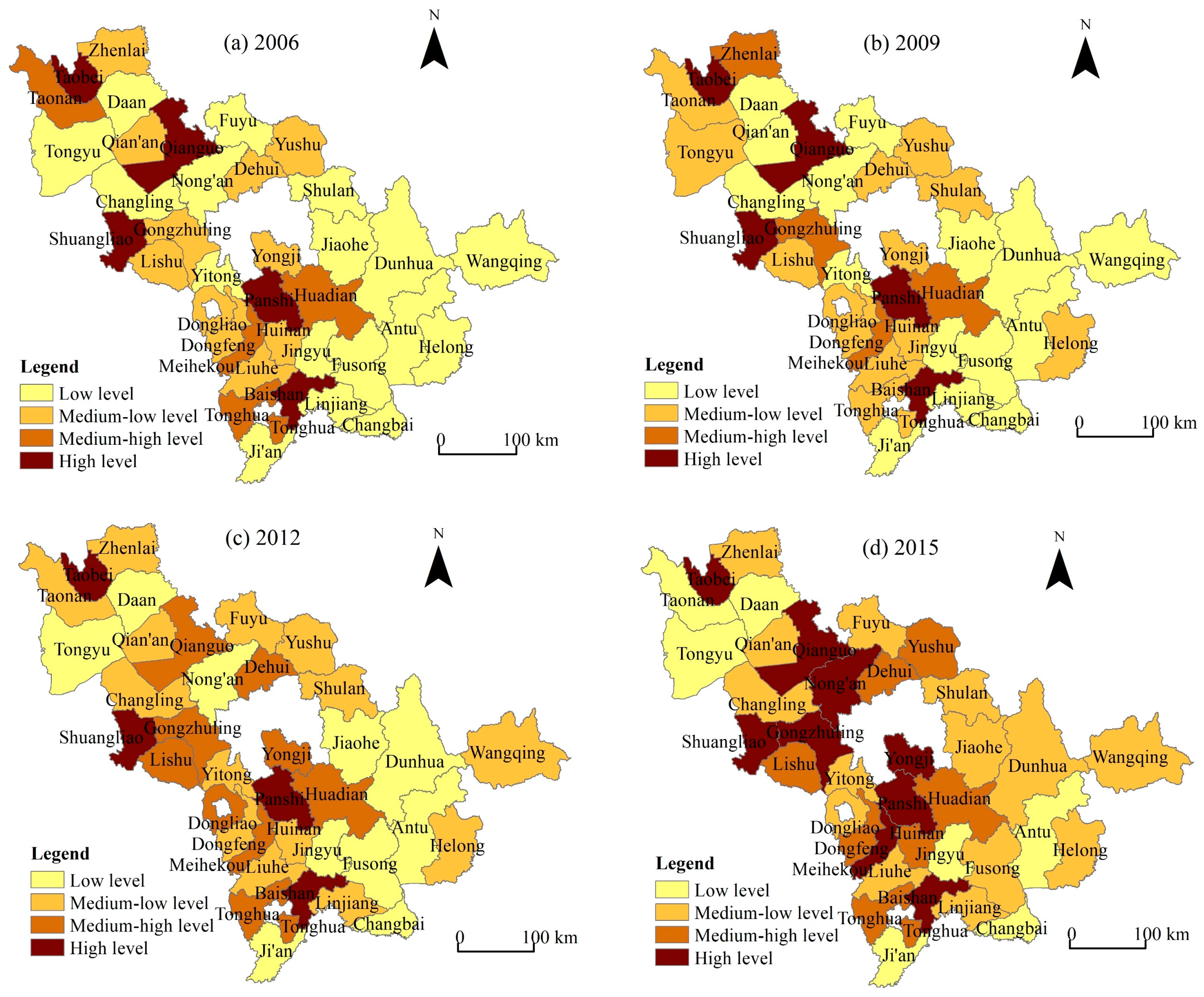
4.2.1. The Spatial Distribution Characteristics of Industrial Pollution Level

To better observe the characteristics of the spatiotemporal evolution, this paper chooses an appropriate time interval (2006, 2009, 2012, and 2015) and then, utilizing the natural break function in ArcGIS 10.2 software, divides the industrial pollution level into four categories: the high level, medium-high level, medium-low level, and low level. As illustrated in Figure 4, the industrial pollution of each county has certain geographical differences and significant spatially polarized characteristics overall in 2006, 2009, 2012, and 2015. Specifically, in 2006, counties with high levels are mainly distributed in Taobei, Qianguo, Panshi, Shuangliao, and Baishan. In these counties, coal, timber, iron ore, and ferrous metal mining industries account for a large share of the industrial economy, leading to heavy-duty secondary industry with obvious characteristics. Taonan, Huadian, Meihekou, and Tonghua have industrial pollution levels that are medium-high. Clearly, counties with low values are also observed in the eastern and southern JRDZ, representing 45.95% of the total. This year, most counties of eastern and southern JRDZ are forestry resource-based cities that face a dilemma of economic transition, leading to lagged industrial development and relatively strong resource constraints. In contrast, in 2009, the distribution of industrial pollution in each county remains relatively stable. Taobei, Qianguo, Panshi, Shuangliao, and Baishan Counties all stay at high levels. The consistent high level industrial pollution in these counties is because of the dominant role in the three industries for a long time. The counties with medium-high industrial pollution levels are Zhenlai, Gongzhuling, Huadian, and Meihekou. Taonan and Tonghua Counties start at the medium-high level and declined to the medium-low level from 2006 to 2009. In 2012, Taobei, Qianguo, Panshi, Shuangliao, and Baishan all stayed at high levels, but Qianguo County did not. These counties have fallen into the trap of a “resource curse” due to their natural resource endowments and oil and gas extraction chemical industry, these counties rely more on the development of high-energy-consuming industries such as chemicals and petroleum, thereby leading to serious industrial pollution emissions and serious pressure on resources and the environment. In 2015, the level of county-level industrial pollution emissions experienced a sharp change with remarkable spatial variations overall, particularly in counties with high and medium-low levels. During this period, the medium-high level is mainly scattered across Deihui, Yushu, Lishu, Huandian, Dongfeng, Huinan, and Tonghua Counties, while there are few counties of this type in 2012. Taonan, Tongyu, Daan, Antu, Jingyu, Changbai, and Ji’an have an industrial pollution level that is at the medium-high level. The number of counties in which the industrial pollution level is high increases while the distribution of the counties with medium-low industrial pollution emissions gradually expands in magnitude. In the areas with medium-low industrial pollution, it may because of the insufficient environmental infrastructure construction, low environmental standards, and extensive operation management. The environmental infrastructure and service facilities are not complete, and the capital investment for the weak links of the environmental infrastructure is insufficient.

4.2.2. The Spatial Distribution Characteristics of the Elastic Decoupling between Industrial Pollution and Economic Growth

To better observe the nexus between industrial pollution and economic growth, this paper calculates the elastic decoupling index and displays the map of spatial distribution in 2006–2007, 2010–2011, and 2014–2015 (Figure 5). In 2006–2007, the types of decoupling between industrial pollution and economic growth are mainly weak decoupling, strong decoupling, expanded-negative decoupling, and expanded connection, accounting for 35.14%, 27.03%, 29.73%, and 0.81%, respectively. The growth rate of 35.14% counties of industrial pollution is much faster than the rate of economic growth. The growth rate of 27.03% counties of industrial pollution is much slower than the rate of economic growth. Of the counties, 30.54% are in an economically unsustainable state. Among them, counties with good decoupling status are mainly located in the southeastern JRDZ, accounting for 62.17%, while other counties have not achieved the decoupling of industrial pollution and economic growth and are still facing economic growth pressure with high environmental pollution. In 2010–2011, the types of decoupling between industrial pollution and economic growth are mainly weak decoupling, strong decoupling, expanded-negative decoupling, and expanded connection, accounting for 13.51%, 27.03%, 54.05%, and 5.41%, respectively. There are 27.03% counties that the growth rate of economic growth is much faster than the rate of industrial pollution, which indicates they are in an economically sustainable state. At the same time, there are 59.46% counties that are in an economically unsustainable state. The spatial distribution area of strong decoupling and weak decoupling has been narrowed and scattered, and only 15 counties have achieved effective decoupling, while the spatial distribution area of expanded-negative decoupling types has further expanded, presenting a contiguous distribution. Combined with expansion connection types, they accounted for a larger proportion of the region, accounting for 59.46%. In 2014–2015, the types of decoupling between industrial pollution and economic growth are mainly debilitating decoupling, weak decoupling, strong decoupling, expanded-negative decoupling and expanded connection, accounting for 13.51%, 37.84%, 8.11%, 37.84%, and 2.7%, respectively. In this period, there are 37.84% counties that are in a strong sustainable state while there are 21.62% that are in an weak sustainable state, which indicates that the growth rate of economic growth is much faster than the rate of industrial pollution. The conflicts between industrial pollution and economic development have been eased and improved. Strong decoupling types are distributed in marginal counties, including Taonan, Da’an, Tongyu, Qian’an, Wangqing, Helong, Antu, Changbai, Ji’an, and other counties, whose decoupling effect of industrial pollution pressure and economic growth is significant.

4.3. Analysis of the Spatial Econometric Estimation Results

The abovementioned explained and explanatory variables are transformed into natural logarithmic form since the untaken natural logarithm data may produce heteroscedasticity in the course of model estimation [42]. Based on the above theoretical analysis, we introduce EDL, PD, UL, TP, IN, ISU, IPC, and EB into formulas (4) and (5); thus, the spatial econometric model (SLM and SEM) is defined as the following Equations (6) and (7):

lnIPI_it = α₀ + α₁lnTP_it + α₂lnEDL_it + α₃lnPD_it + α₄lnUL_it + α₅lnIN_it + α₆lnISU_it + α₇lnIPC_it + α₈lnEB_it + ρW_itIPI_it + ε_it

(6)

lnIPI_it = β₀ + α₁lnTP_it + β₂lnEDL_it + β₃lnPD_it + β₄lnUL_it + β₅lnIN_it + β₆lnISU_it + β₇lnIPC_it + α₈lnEB_it + ε_it, ε_it = λW_itIPI_it + u_it

(7)

where IPI denotes the industrial pollution index, TP denotes technological progress, EDL represents the economic development level, PD represents population density, UL denotes the urbanization level, IN represents industrialization, ISU denotes industrial structure upgrading, IPC denotes industrial production capacity, and EB represents the ecological base.

4.3.1. Spatial Autocorrelation Test

A spatial autocorrelation test is required, and the Moran’s I values are obtained employing STATA 15.0 software (

Table 2. The trend of the Moran’s I of the industrial pollution index in the JRDZ.

Year	2006	2007	2008	2009	2010	2011	2012	2013	2014	2015
Moran’s I	0.194	0.192	0.186	0.169	0.182	0.181	0.223	0.176	0.198	0.179
E(I)	−0.028	−0.028	−0.028	−0.028	−0.028	−0.028	−0.028	−0.028	−0.028	−0.028
Z-value	1.833	1.825	1.792	1.651	1.752	1.730	2.089	1.693	1.878	1.710
P	0.067	0.068	0.073	0.099	0.080	0.084	0.037	0.090	0.060	0.087

). As displayed in Table 2, the Moran’s I values for the observation period are above 0, ranging from 0.169 to 0.223. In addition, the Z-values exceeding 1.65 are all statistically significant at the 10% level, indicating that there exists significant positive spatial autocorrelation of the industrial pollution index and that the geographical distribution of the industrial pollution index tends show clustering, which also fully demonstrates the spatial disparities in industrial pollution among counties with higher spatial autocorrelation. Specifically, such findings demonstrate that there exists a significant spatial agglomeration effect of the industrial pollution index from 2006 to 2015. If the industrial pollution index of one county is high, then so is that of its neighboring counties. For yearly variation, the overall trend tends to be relatively stable, with values ranging from 0.169 to 0.223, demonstrating that the spatial agglomeration effect maintains a smooth and steady trend overall. From the perspective of the maximum and minimum values, the highest clustering intensity is observed in 2012, while the lowest is found in 2009. We can attribute this finding to the following reasons. In 2009, the implementation of Jilin revitalization policy promotes the obvious transformation of industrial structure, and the enterprises have started to focus on the full implementation of clean production, thus leading the relatively low clustering intensity of industrial pollution among counties. As the economic pressure was relatively high in 2012, the industrial economy was transformed from scale to intensive and strengthened the dominant role of industry, thereby leading to the acceleration of natural resource consumption and more serious industrial pollution. Thus, the clustering intensity of industrial pollution in 2012 is the highest.

4.3.2. Spatial Econometric Regression Estimation

Based on the analysis above, the characteristics of the spatial agglomeration of the industrial pollution index are prominent during the observation period. Next, we apply the spatial econometric regression estimation to illustrate the driving factors of the industrial pollution index and, based on the spatial weight matrix, construct an SLM and an SEM that do not investigate the spatial factors that will fail. As proposed by the previous literature, the Lagrange multiplier (LM) and robust Lagrange multiplier (R-LM) can provide guidance to assess whether the SLM or the SEM is the most appropriate model for estimation by comparing the significance of the LM and R-LM at the 1% level. Based on this step, the Hausman test is generally applied to determine whether a random effect model or a fixed effect model is suitable for the estimation results through maximum likelihood estimation. We apply MATLAB (R2016a) software to operate the panel data spatial econometric model code compiled by Elhorst [43]. According to the results obtained, the values of LM-lag, R-LM-lag, and LM-error are 7.2889, 4.7282, and 3.8903, respectively, and all are significant at the 10% level, while the value of R-LM-error is 1.3296 and is not significant at the 10% level. These results demonstrate that the LM test result of the SLM is more significant than that of the SEM, while the R-LM test result of the SLM is significant, but that of the SEM is not. Therefore, these results fully indicate that the SLM is more suitable for estimating industrial emission factors than the SEM. As the Hausman test results are 32.923 with a p value of 0.000, we reject the null hypothesis to regress the SLM with the fixed effect. Accordingly, the fixed effect model of the SLM is selected as the appropriate model for elaborating the influencing factors of industrial pollution.

4.3.3. Results Analysis

The empirical results obtained from the spatial econometric estimation and the ordinary least squares (OLS) are presented in

Table 3. Regression results of the spatial econometric model.

Explanatory Variables	OLS		SLM-FE		SEM-FE
	Coeff.	t	Coeff.	t	Coeff.	t
lnEDL	−0.317 **	−2.070	−0.496 **	−2.196	−0.506 **	−2.230
lnPD	0.481 ***	5.693	0.243 **	−2.121	0.258 **	−2.137
lnUL	0.258 ***	3.136	0.037	0.617	0.0393	0.652
lnTP	0.024	0.499	−0.073 *	−1.713	−0.074 *	−1.733
lnIN	0.647 ***	4.674	−0.352 **	−2.106	−0.350 **	−2.085
lnISU	−0.438 *	−1.890	−0.298	−1.184	−0.301	−1.199
lnIPC	0.236 **	2.063	0.476 ***	3.521	0.477 ***	3.531
lnEB	0.330 ***	5.369	0.080	0.274	0.081	0.279
intercept	−6.348 ***
Log-like.	−476.1641		−218.5405		−218.9689
R2	0.4452		0.8129		0.8119

***, ** and * indicate significance at the 1%, 5% and 10% levels.

. The R² of the SLM with the fixed effect model (SLM-FE) is 0.8129, which indicates that the goodness of fit of the model equation is ideal. As shown in Table 3, EDL, PD, TP, IN, and IPC are all statistically significant at the 10% level, demonstrating that these five selected variables have strong explanatory power in regard to industrial pollution. Specifically, the SLM-FE results reveal that the economic development level (EDL), technological progress (TP), and industrialization (IN) exert a significant negative effect on industrial pollution emissions, while population density (PD) and industrial production capacity (IPC) positively influence industrial pollution emissions. The coefficient of the urbanization level (UL) turns out to be positive but statistically nonsignificant, and it is uncertain whether the degree of industrial structure upgrading (ISU) is suppressed by the level of industrial pollution emissions due to the nonsignificant t values.

The economic development level (EDL), measured by per capita GDP, is negatively associated with industrial pollution emissions, and the coefficient of the economic development level is significant at the 5% level. This result indicates that a 1% increase in the economic development level will lead to a 0.496% decrease in industrial pollution emissions when all other variables are fixed. The economic development level tends to curb and mitigate the increase in industrial pollution emissions. Many empirical studies have reached the consensus that pollution emissions vary nonlinearly in different economic level stages. In our explanation, the counties in which per capita GDP is very high are also likely to generally focus more on the quality of the ecological environment as the residents’ material living conditions rapidly improve. In addition, their governments have more financial resources and labor to invest in energy-saving and environmental protection actions, which will also mitigate industrial environmental pollution. In other words, when per capita GDP greatly increases, industrial pollution emissions are likely to ultimately decrease.

The correlation coefficient between population density (PD) and industrial pollution emissions is positive and statistically significant at the 5% level, demonstrating that a 1% increase in population density can increase industrial pollution emissions by 0.243% when all other variables are fixed. The results indicate that improving the population density tends to intensify industrial pollution emissions when all other variables are fixed. The reason is that the dramatic expansion of counties is likely to create an intense need for the energy and resources necessary to meet the demands of economic development, leading to greater social conflict over pollutant emissions and the materials for production and living. Intuitively, industrial pollutant emissions have a strong pollution attribute and industrial orientation, and they may be affected more by the industrial layout than by the population density. The population density estimation results provide strong evidence supporting Selden and Song, who show that there is more pressure to impose strict environmental regulation in counties with a high population density for curbing industrial pollution emissions because of the high industrial pollution [44].

Regarding industrialization (IN), the correlation coefficient is −0.352 and significant at the 5% level, which means that a 1% increase in industrialization can curb industrial pollution emissions by 0.352% when all other variables are fixed. Notably, this finding is not consistent with that of Dong et al. [45], who confirmed that industrialization is a vital positive determinant of environmental pollution. Under the pressure of environmental regulation, each county implements a blacklist of industrial access, sets strict conditions for industrial access, restricts the categories of industrial development, clearly restricts or prohibits industries, and strictly controls the industry in areas such as coal and iron production that do not meet the development control principles of restricted development zones. The government and enterprises upgrade, shut down, and transfer existing environmentally polluting enterprises, implement industrial admission, and thus suppress industrial pollutant emissions.

As demonstrated by the estimation results in Table 3, technological progress (TP) contributes to a decrease in industrial pollution emissions when all other variables are fixed. The correlation coefficient between technological progress and industrial pollution emissions is −0.073, indicating that a 1% increase in technological progress causes an approximately 0.073% reduction in industrial pollution emissions when all other variables are fixed. The correlation coefficient of technological progress is not huge, but it is large enough to have an impact. This result directly confirms the fact that financial expenditure on science and technology is an important means for counties to promote scientific and technological progress. Specifically, although technological advances probably bring a considerable amount of industrial pollution as the production scale expands, conversely, they will stimulate the potential innovation of industrial production, generate a rebound effect, lead to an increase in the efficiency of resource use and make the enterprises that introduce innovation profit from clean production technology, which will inevitably reduce industrial pollutants at the same time. In other words, counties with more sufficient financial investment support for pollution mitigation technology have the ability to curb increases in industrial pollution emissions.

In contrast to the correlation coefficient of the above factors, the correlation coefficient of industrial production capacity (IPC) is positive and significant, indicating that industrial production capacity has a positive correlation with industrial pollution emissions. A 1% increase in industrial production capacity can increase industrial pollution emissions by 0.476% when all other variables are fixed. This conclusion is directly correlated with the fact that industrial enterprises with high production capacity are more likely to access distinct advantages, especially in labor, information, technology, capital, and resources, resulting in an increase in energy consumption and industrial pollution emissions, which to some extent may produce high industrial pollution emissions. Hence, it is not difficult to understand that counties with enterprises whose production capacity value is above the designated size have a more serious industrial pollution situation.

5. Conclusions and Policy Suggestions

Our research conclusions will help improve our understanding of the dynamics of pollution emissions during the 2006–2015 period and offer a policy basis for different types of counties to implement differentiated prevention strategies that are useful for environmental improvement and pollutant emission reduction.

5.1. Conclusions

By comprehensively taking into account six industrial pollutants, this paper provides empirical evidence for investigating the characteristics of the temporal evolution and spatial pattern of the industrial pollution index and its socioeconomic influencing factors. In this paper, the empirical conclusions reveal the following. The temporal evolution of the industrial pollution index of the JRDZ is generally characterized by a trend of first decreasing and then increasing. The industrial pollution index has certain geographical differences and prominent spatially polarized characteristics overall in 2006, 2009, 2012, and 2015. There is mostly a significant positive spatial autocorrelation of the industrial pollution index, and the geographical distribution of the industrial pollution index tends to show clustering. Spatial regression models that incorporate spatial factors better explain the influencing factors of industrial pollution emissions. The economic development level, technological progress, and industrialization contribute to curbing industrial pollution emissions, while population density and industrial production capacity exert a significant enhancement effect that positively influences industrial pollution emissions.

5.2. Policy Suggestions

Based on the conclusions drawn from our empirical evidence, several relevant policy recommendations can be proposed to control industrial pollution emissions. First, concerning the findings of the distribution of emissions in the JRDZ, the prominent spatial disparities in industrial pollution emissions across different counties indicate that industrial pollution reduction policies should be distinct and implemented based on current developmental stages and location conditions. Second, the spatial autocorrelation tests demonstrated that the spatial dependence of environmental pollution levels in Jilin Province experienced a nonobvious-to-obvious evolutionary process within the study period. Significant spatial autocorrelation effects on industrial pollution should be taken into account before formulating industrial emission reduction policies, which illustrates that it is essential to give full play regional cooperation in curbing industrial emissions. Therefore, to more effectively avoid environmental risks, the government should establish and improve the linkage mechanisms of interregional joint prevention. Third, the estimation results of the determinant factors demonstrate several measures to curb industrial pollution in the JRDZ based on the following. In addition, the result that technological progress contributes to curbing the increase in industrial pollution emissions reveals that the government should give full play to the supporting role of technological innovation in industrial emission reduction, promote the technological transformation of technological achievements, and build a green technology innovation system via a policy of innovation incentives. Furthermore, enterprises should continuously update their environmental protection methods (e.g., resource-efficient technology, cleaner production technology, recycling technology, and pollution control technology) in the process of pollution control, thereby forcing regional industrial development to meet the goal of environmental quality protection and friendliness. Moreover, this study finds that industrialization contributes to curbing industrial pollution, indicating that the government should increase the elimination of outdated production capacity in key industries such as iron and steel production and encourage local governments to designate policies for eliminating outdated production capacity with a wider scope and stricter standards. The government should also conduct environmental assessments on key industries and the industrial layout, raise pollution emission standards, strengthen the environmental governance of air, water, soil and solid waste, build a complete environmental protection credit system, strengthen the environmental protection credit evaluation and information disclosure system, and strengthen the main responsibilities of polluters. Industrial production capacity also has a positive effect on industrial emissions. Accordingly, the government should adjust and optimize industrial layouts, scales, and structures that do not conform to the functional positioning of the ecological environment. Furthermore, the government should eliminate the backward production capacity of industrial enterprises, relocate and close heavily polluting enterprises, actively guide and support the development of the environmental protection industry, and focus on supporting the development of resource-saving and environmentally friendly replacement industries, such as ecotourism, tertiary industries, and green industries. The government should compile and formulate an ecological access list and industry access blacklist, strictly restrict and control the production capacity of “high pollution and high emissions” industries, and cultivate industries that are consistent with the development direction and development control principles. The JRDZ should thoroughly implement the concept of green development, pay more attention to the copreservation of ecological space and cogovernance of environmental pollution, and promote the establishment of ecological compensation and pollution compensation mechanisms.

Overall, there remain several limitations that must be further addressed, although the conclusions provide a series of corresponding policy suggestions for environmental managers. Since the theoretical process of the dynamic mechanism is complicated and cumbersome, it is necessary to comprehensively consider various factors and data support. Due to the limitations of current statistical data disclosed to the public, energy consumption data, FDI data, and specific subsector data were not considered in our analysis of influencing factors, which is also a problem that we need to solve in further in-depth research.

References

1. Wang, M.; Webber, M.; Finlayson, B.; Barnett, J. Rural industries and water pollution in China. J. Environ. Manag. 2008, 86, 648–659. [Google Scholar] [CrossRef]
2. Dimitriou, K.; Paschalidou, A.K.; Kassomenos, P.A. Assessing air quality with regards to its effect on human health in the European Union through air quality indices. Ecol. Indic. 2013, 27, 108–115. [Google Scholar] [CrossRef]
3. Batisse, E.; Goudreau, S.; Baumgartner, J.; Smargiassi, A. Socio-economic inequalities in exposure to industrial air pollution emissions in Quebec public schools. Can. J. Public Health 2017, 108, 503–509. [Google Scholar] [CrossRef] [PubMed] [Green Version]
4. Fan, J.; Li, P. The scientific foundation of major function oriented zoning in China. J. Geogr. Sci. 2009, 19, 515. [Google Scholar] [CrossRef]
5. Wang, Y.F.; Fan, J. Multi-scale analysis of the spatial structure of China’s major function zoning. J. Geogr. Sci. 2020, 30, 197–211. [Google Scholar] [CrossRef]
6. Tobey, J.A. Economic development and environmental management in the Third World: Trading-off industrial pollution with the pollution of poverty. Habitat Int. 1989, 13, 125–135. [Google Scholar] [CrossRef]
7. Ray, S.; Kim, K.H. The pollution status of sulfur dioxide in major urban areas of Korea between 1989 and 2010. Atmos. Res. 2014, 147, 101–110. [Google Scholar] [CrossRef]
8. Barron, W.F. Evaluating alternative environmental control measures: The case of industrial sulfur dioxide in Hong Kong. J. Environ. Manag. 1992, 35, 229–238. [Google Scholar] [CrossRef]
9. Teng, X.; Lu, L.; Chiu, Y.H. Considering emission treatment for energy-efficiency improvement and air pollution reduction in China’s industrial sector. Sustainability 2018, 10, 4329. [Google Scholar] [CrossRef] [Green Version]
10. Hang, Y.; Wang, Q.; Wang, Y.; Su, B.; Zhou, D. Industrial SO2 emissions treatment in China: A temporal-spatial whole process decomposition analysis. J. Environ. Manag. 2019, 243, 419–434. [Google Scholar] [CrossRef]
11. Li, H.; Ma, Y.; Duan, F.; He, K.; Zhu, L.; Huang, T.; Takashi, K.; Ma, X.; Ma, T.; Xu, L.; et al. Typical winter haze pollution in Zibo, an industrial city in China: Characteristics, secondary formation, and regional contribution. Environ. Pollut. 2017, 229, 339–349. [Google Scholar] [CrossRef]
12. Wang, J.; Xie, X.; Fang, C. Temporal and spatial distribution characteristics of atmospheric particulate matter (PM10 and PM2.5) in Changchun and analysis of its influencing factors. Atmosphere 2019, 10, 651. [Google Scholar] [CrossRef] [Green Version]
13. Wang, C.; Du, X.; Liu, Y. Measuring spatial spillover effects of industrial emissions: A method and case study in Anhui province, China. J. Clean. Prod. 2017, 141, 1240–1248. [Google Scholar] [CrossRef]
14. Song, C.; Wu, L.; Xie, Y.; He, J.; Chen, X.; Wang, T.; Lin, Y.; Jin, T.; Wang, A.; Liu, Y.; et al. Air pollution in China: Status and spatiotemporal variations. Environ. Pollut. 2017, 227, 334–347. [Google Scholar] [CrossRef]
15. Li, L.; Qian, J.; Ou, C.Q.; Zhou, Y.X.; Guo, C.; Guo, Y. Spatial and temporal analysis of Air Pollution Index and its timescale-dependent relationship with meteorological factors in Guangzhou, China, 2001–2011. Environ. Pollut. 2014, 190, 75–81. [Google Scholar] [CrossRef]
16. Chen, J.; Chen, K.; Wang, G.; Wu, L.; Liu, X.; Wei, G. PM2.5 pollution and inhibitory effects on industry development: A bidirectional correlation effect mechanism. Int. J. Environ. Res. Public Health 2019, 16, 1159. [Google Scholar] [CrossRef] [Green Version]
17. Li, M.; Wang, L.; Liu, J.; Gao, W.; Song, T.; Sun, Y.; Li, L.; Li, X.; Wang, Y.; Liu, L.; et al. Exploring the regional pollution characteristics and meteorological formation mechanism of PM2.5 in North China during 2013–2017. Environ. Int. 2020, 134, 105283. [Google Scholar] [CrossRef] [PubMed]
18. Köne, A.Ç.; Büke, T. The evaluation of the air pollution index in Turkey. Ecol. Indic. 2014, 45, 350–354. [Google Scholar] [CrossRef]
19. Halkos, G.E.; Polemis, M.L. The impact of economic growth on environmental efficiency of the electricity sector: A hybrid window DEA methodology for the USA. J. Environ. Manag. 2018, 211, 334–346. [Google Scholar] [CrossRef]
20. Tachie, A.K.; Xingle, L.; Dauda, L.; Mensah, C.N.; Appiah-Twum, F.; Mensah, I.A. The influence of trade openness on environmental pollution in EU-18 countries. Environ. Sci. Pollut. Res. 2020, 27, 35535–35555. [Google Scholar] [CrossRef] [PubMed]
21. He, J. Pollution haven hypothesis and environmental impacts of foreign direct investment: The case of industrial emission of sulfur dioxide (SO2) in Chinese provinces. Ecol. Econ. 2006, 60, 228–245. [Google Scholar] [CrossRef] [Green Version]
22. He, J. China’s industrial SO2 emissions and its economic determinants: EKC’s reduced vs. structural model and the role of international trade. Environ. Dev. Econ. 2009, 14, 227–262. [Google Scholar] [CrossRef]
23. Sanchez, L.F.; Stern, D.I. Drivers of industrial and non-industrial greenhouse gas emissions. Ecol. Econ. 2016, 124, 17–24. [Google Scholar] [CrossRef] [Green Version]
24. He, Z.; Shi, X.; Wang, X.; Xu, Y. Urbanisation and the geographic concentration of industrial SO2 emissions in China. Urban Stud. 2017, 54, 3579–3596. [Google Scholar] [CrossRef]
25. Zhou, Y.; Zhu, S.; He, C. How do environmental regulations affect industrial dynamics? Evidence from China’s pollution-intensive industries. Habitat Int. 2017, 60, 10–18. [Google Scholar] [CrossRef] [Green Version]
26. Jiao, J.; Han, X.; Li, F.; Bai, Y.; Yu, Y. Contribution of demand shifts to industrial SO2 emissions in a transition economy: Evidence from China. J. Clean Prod. 2017, 164, 1455–1466. [Google Scholar] [CrossRef]
27. Li, M.; Li, C.; Zhang, M. Exploring the spatial spillover effects of industrialization and urbanization factors on pollutants emissions in China’s Huasng-Huai-Hai region. J. Clean. Prod. 2018, 195, 154–162. [Google Scholar] [CrossRef]
28. Zhu, L.; Hao, Y.; Lu, Z.N.; Wu, H.; Ran, Q. Do economic activities cause air pollution? Evidence from China’s major cities. Sust. Cities Soc. 2019, 49, 101593. [Google Scholar] [CrossRef]
29. Chen, S.; Zhang, Y.; Zhang, Y.; Liu, Z. The relationship between industrial restructuring and China’s regional haze pollution: A spatial spillover perspective. J. Clean. Prod. 2019, 239, 115808. [Google Scholar] [CrossRef]
30. Liu, Y.; Wang, S.; Qiao, Z.; Wang, Y.; Ding, Y.; Miao, C. Estimating the dynamic effects of socioeconomic development on industrial SO2 emissions in Chinese cities using a DPSIR causal framework. Resour. Conserv. Recycl. 2019, 150, 104450. [Google Scholar] [CrossRef]
31. Liu, K.; Lin, B. Research on influencing factors of environmental pollution in China: A spatial econometric analysis. J. Clean. Prod. 2019, 206, 356–364. [Google Scholar] [CrossRef]
32. Grossman, G.M.; Krueger, A.B. Economic growth and the environment. Q. J. Econ. 1995, 110, 353–377. [Google Scholar] [CrossRef] [Green Version]
33. Hosseini, H.M.; Kaneko, S. Can environmental quality spread through institutions? Energy Policy 2013, 56, 312–321. [Google Scholar] [CrossRef]
34. Liu, Y.; Zhou, Y.; Wu, W. Assessing the impact of population, income and technology on energy consumption and industrial pollutant emissions in China. Appl. Energy 2015, 155, 904–917. [Google Scholar] [CrossRef]
35. Yang, Y.; Zhao, T.; Wang, Y.; Shi, Z. Research on impacts of population-related factors on carbon emissions in Beijing from 1984 to 2012. Environ. Impact Assess. Rev. 2015, 55, 45–53. [Google Scholar] [CrossRef]
36. Hao, Y.; Liu, Y.; Weng, J.H.; Gao, Y. Does the Environmental Kuznets Curve for coal consumption in China exist? new evidence from spatial econometric analysis. Energy 2016, 114, 1214–1223. [Google Scholar] [CrossRef]
37. Shen, J.; Wang, S.; Liu, W.; Chu, J. Does migration of pollution-intensive industries impact environmental efficiency? Evidence supporting “Pollution Haven Hypothesis”. J. Environ. Manag. 2019, 242, 142–152. [Google Scholar] [CrossRef]
38. Wei, D.; Liu, Y.; Zhang, N. Does industry upgrade transfer pollution: Evidence from a natural experiment of Guangdong province in China. J. Clean. Prod. 2019, 229, 902–910. [Google Scholar] [CrossRef]
39. Tapio, P. Towards a theory of decoupling: Degrees of decoupling in the EU and the case of road traffic in Finland between 1970 and 2001. Transp. Policy 2005, 12, 137–151. [Google Scholar] [CrossRef] [Green Version]
40. Moran, P.A. The interpretation of statistical maps. J. R. Stat. Soc. Ser. B 1948, 10, 243–251. [Google Scholar] [CrossRef]
41. Anselin, L. Spatial Econometrics: Methods and Models; Kluwer Academic Publishers: Dordrecht, The Netherlands, 1988. [Google Scholar]
42. Elhorst, J.P. The mystery of regional unemployment differentials: Theoretical and empirical explanations. J. Econ. Surv. 2003, 17, 709–748. [Google Scholar] [CrossRef]
43. Elhorst, J.P. Matlab software for spatial panels. Int. Reg. Sci. Rev. 2014, 37, 389–405. [Google Scholar] [CrossRef] [Green Version]
44. Selden, T.M.; Song, D. Environmental quality and development: Is there a Kuznets curve for air pollution emissions? J. Environ. Econ. Manag. 1994, 27, 147–162. [Google Scholar] [CrossRef]
45. Dong, K.; Hochman, G.; Kong, X.; Sun, R.; Wang, Z. Spatial econometric analysis of China’s PM10 pollution and its influential factors: Evidence from the provincial level. Ecol. Indic. 2019, 96, 317–328. [Google Scholar] [CrossRef]
Figure 1. Map of the study area.
Sustainability 13 04194 g001
Figure 2. The overall temporal trend of industrial pollution intensity in 2006–2015.
Sustainability 13 04194 g002
Figure 3. The average industrial pollution level for the JRDZ in 2006–2015.
Sustainability 13 04194 g003
Figure 4. The spatial pattern characteristics of industrial pollution for the JRDZ in 2006–2015.
Sustainability 13 04194 g004
Figure 5. The spatial pattern characteristics of industrial pollution for the JRDZ in 2006–2015.
Sustainability 13 04194 g005