Comparison of Logistic Regression, Information Value, and Comprehensive Evaluating Model for Landslide Susceptibility Mapping

Abstract

This study validated the robust performances of the recently proposed comprehensive landslide susceptibility index model (CLSI) for landslide susceptibility mapping (LSM) by comparing it to the logistic regression (LR) and the analytical hierarchy process information value (AHPIV) model. Zhushan County in China, with 373 landslides identified, was used as the study area. Eight conditioning factors (lithology, slope structure, slope angle, altitude, distance to river, stream power index, slope length, distance to road) were acquired from digital elevation models (DEMs), field survey, remote sensing imagery, and government documentary data. Results indicate that the CLSI model has the highest accuracy and the best classification ability, although all three models can produce reasonable landslide susceptibility (LS) maps. The robust performance of the CLSI model is due to its weight determination by a back-propagation neural network (BPNN), which successfully captures the nonlinear relationship between landslide occurrence and the conditioning factors.

1. Introduction

In terms of economic and death impact, landslides rank seventh globally [1]; they cause damage to roads, railways, power lines, and even tourism and historical sites [2,3]. China is a mountainous country, with its development severely restricted by landslides. Many efforts have been made to prevent and alleviate landslides. Landslide hazard is characterized by two main components: the first is temporal, related to landslide frequency in a particular area; the second one is spatial and is related to the spatial probability of occurrence of landslides, so-called “susceptibility” [4]. Landslide susceptibility mapping (LSM) is critical for landslide prevention [5,6]. Herein, the main points of landslide susceptibility mapping are simply summarized: first, the conditioning factors (CFs) and their contributions are determined by analyzing the characteristics and distribution of the existing landslides; after that, through a linear or nonlinear way, the relationship between CFs and landslide susceptibility is established; finally, using the relationship, LSM for unknown areas can be completed [7]. LSM is the spatial assessment of landslide at initial stage. Its accuracy directly affects the rationality of the site selection as well as the decision of the disaster control. Therefore, LSM has vital practical significance.

The research techniques used for LSM can be roughly categorized into qualitative and quantitative ones [8,9]. The qualitative methods are based on prior knowledge of experts. The basic idea of the qualitative method is that experts identify the judgment rules for conditioning factors and then perform a weighted summation of them to obtain the landslide susceptibility map [10]. The most representative and widely used qualitative method is the analytical hierarchy process (AHP) [11,12,13,14].

The quantitative methods are based on field data. They involve deterministic and statistical approaches. The deterministic model is to judge the stability of slope based on the physical model. It only can be used in areas where the geomorphic and geologic properties are fairly homogeneous [8,15]. The statistical approaches rely on the relationships (linear or nonlinear) between conditioning factors and existing landslides. Lazzari and Danese [4] summarized their scope of application: the qualitative methods are suited for regional surveys at a small scale, the statistical quantitative methods are suited for a medium scale survey, while the deterministic approach is suited for detailed studies at a large scale. Around the 1990s, geographic information system (GIS) and digital terrain data were popularized globally. Thanks to robust scientific advances, a significant boost has been gained in the field of LSM. Nowadays, the combination of GIS and statistical methods is the general way for LSM. Various statistical methods have been used for LSM, including: frequency ratio (FR) [10,16,17,18,19], information value (IV) [20,21], logistic regression (LR) [22,23], back-propagation artificial neural networks [5,24], support vector machine [15,25], extreme learning machine [26,27], probabilistic approach [28], and deep learning algorithm [26,29].

In the past decade, scholars have tried to combine the advantages of different methods to improve the performance of LSM in terms of accuracy and classification ability. The integrated methods commonly seen in the literature are analytical hierarchy process information value (AHPIV) [8], analytical hierarchy process frequency ratio (AHPFR) [30], and integration of the statistical index method and the analytic hierarchy process [31], logistic regression frequency ratio (LRFR) [32,33], logistic regression information value (LRIV) [8,34], the integration of convolutional neural network and conventional machine learning classifiers [35], and integration of kernel density estimation and nearest neighbor methods [4]. However, whether these methods are superior requires further verifications.

The variety of LSM models evokes comparative research between different models. By comparing the three models, Kanungo et al. [36] confirmed that the LSM results using the combined artificial neural networks (ANN) and fuzzy weighting were significantly better than the independent use of the ANN model and fuzzy model. The very high susceptibility zone, although with the least percentage, contained the highest percentage of the existing landslide area. Chen et al. [37] compared the information value (IV) model and LR model, and concluded that the IV model is better in the research area. To confirm that different sampling methods can affect the accuracy of LSM, Nefeslioglu et al. [38] compared the LR method and back-propagation neural network (BPNN) model. The results show that the BPNN algorithms overreacted to the sampling strategy, but this result needed further verification. Comparing three commonly used LSM models: frequency ratio (FR), ANNs, and LR, Pradhan et al. [16] and Yilmaz et al. [39] both concluded that the results by ANNs are better than those by the other two. Pradhan et al. [16] further confirmed that there is no positive linear correlation between the number of CFs and the results’ quality. More importantly, determining the CFs that play a control role is the key to improving the accuracy of LSM [40]. Interestingly, in the same year, Poudyal et al. [17] also compared the FR model and ANN model, and they concluded that the FR model is better than the ANN model in terms of prediction accuracy. In addition to ANNs, other data-driven methods have also attracted extensive attention. Bui et al. [15] found that the LSM results obtained by a support vector machine (SVM) have the best performance, compared to the decision tree and Naïve Bayes. They further explored some new sophisticated machine learning techniques [41], such as multi-layer perceptron neural networks, kernel LR method, etc. In terms of prediction capability, the multi-layer perceptron neural networks model performed best. Nowadays, comparative research on landslide susceptibility mapping models has never stopped [3,29,42,43,44].

The first author has proposed an integrated model for LSM [6], which is an integration of the prior knowledge and the objective weighting method. The model integrates several methods: frequency ratio (FR) method, cluster analysis (CA), and back-propagation neural networks (BPNNs). The FR method is used to determine the weighted value for each class of the conditioning factors of landslide, the BPNN is utilized to determine the weighted value for every factor, and the CA is used to optimize the non-landslide samples before the BPNN process. For convenience, this model is denoted as the CLSI model, which is the abbreviation of the comprehensive landslide susceptibility index [45] model.

To further verify the superiority and generalizability of this model, Zhushan County was taken as a study region. It is a landslide-prone area in Hubei Province of China.

Two representative methods, namely, the LR and the analytic hierarchy process information value (AHPIV) model, were used for comparison. Specifically, LR represents the traditional statistical method, and AHPIV represents an integrated method that combines prior knowledge and subjective weight determination. With these methods, the landslide susceptibility (LS) maps of the study region were produced, respectively, and their performances were evaluated in terms of prediction accuracy and classification ability. The verification methods included the area under the receiver operating feature curve (AUC), seed cell area index (SCAI), and the cumulative number of landslide points.

2. Methodology

2.1. LR Model

The LR is one of the most common statistical methods in earth sciences [39]. The variables in the LR model can be either discrete or continuous. For continuous variables, normal distributions are not required [18]. This feature is quite useful in LSM due to the diversity and complexity of CFs [46].

In the LR model, the relationship between landslide occurrence and the CFs can be described as [37]:

$$P=\frac{1}{1+e^{-Z}}$$

(1)

where P (0 ≤ P ≤ 1) is the probability of landslide occurrence, meanwhile, Z is linear logistic parameter Logit (P) with the range of $\left(-\infty ,+\infty \right)$. Equation (2) shows the detailed calculation of Z [2].

$$Z=Logit\left(P\right)=\ln (\frac{P}{1-P})={\beta }_0+{\beta }_1{x}_1+\cdots +{\beta }_n{x}_n$$

(2)

where n is the quantity of landslide CFs, β₀ the constant coefficient, β₁ …β_n the partial regression coefficients, and x₁…x_n the independent variables (i.e., the CFs in this study).

2.2. AHPIV Model

The AHPIV model is an integrated model that can be expressed by a weighted sum equation [8]:

$$I_n={\displaystyle \sum }_{i=1}^n{w}_i{I}_i$$

(3)

where w_i is CF weights and I_i is the information value (IV) of the CF class. In the AHPIV, the AHP is used to obtain the w_i, and the information value method is used to obtain the I_i. The two methods are briefly described as follows.

2.2.1. AHP Method

The AHP is a semi-qualitative multi-criteria decision-making technique, which is widely used in many research fields including LS. It can consider both subjective and objective factors while making the decision [31,43]. It can be used alone [43,47] or in combination with other methods [8] in the LSM.

Using the AHP to determine the weights of CFs, the following steps are involved: (i) build a hierarchy model of factors; (ii) establish a judgment matrix through pairwise comparison (represent the importance from less to more using 1 to 9); (iii) calculate the principal eigenvalue (λ_max) and the corresponding eigenvector of the judgment matrix; (iv) test consistency using the consistency ratio (CR) (see Equation (4)) [48]. CR must be less than 0.1; (v) normalize principal eigenvector to obtain factor weights. In Equation (4), RI is the random consistency index see

Table 1. Random consistency index (RI) [48,49].

n	1	2	3	4	5	6	7	8	9	10	11	12	13	14	15
RI	0	0	0.58	0.90	1.12	1.24	1.32	1.41	1.45	1.49	1.51	1.53	1.56	1.57	1.59

[48,49], and n is the order of the judgment matrix.

$$CR=\frac{CI}{RI}=\left(\frac{{\lambda }_{\max }-n}{n-1}\right)/RI$$

(4)

2.2.2. IV Method

Information value (IV) is an indirect conventional statistical method for LSM [37,43,50]. An information value I_i of a CF class can be defined as [43]:

$$I_i={\log }_2\frac{L_{im}/T_{im}}{L/T}$$

(5)

where L_im is the number of landslide grid cells in $m$th class of ith factor, T_im is the number of the grid cells in $m$th class of ith factor, L is the total number of landslide grid cells, and T is the total number of grid cells in the study area.

The existence of a CF class is adverse to landslide development when I_i is negative; the existence of a CF class is conducive to landslide development when I_i is positive [51].

2.3. The Comprehensive Evaluating (CLSI) Model

Similar to the AHPIV model, the comprehensive evaluating (CLSI) model is also an integrated model [6]. The main purpose of the CLSI model is to calculate the “LSI” of each grid cell [46] see Equation (6).

$$LSI={\displaystyle \sum }_{i=1}^n{w}_i{R}_{im}$$

(6)

where w_i denotes CF weights and R_im denotes the frequency ratio (FR). In the CLSI, the BPNN is applied to obtain w_i, and the FR method is used to evaluate R_im. The two methods are briefly described as follows.

2.4. BPNN Method

The BPNN model commonly includes three layers (input, hidden, and output layers) [43]. The quantized values of the CFs form the input layer, and the absence or presence of landslide, represented by 0 or 1, respectively, is within the output layer. Neurons in these layers are connected to each other by weight values [43]. During training, the networks can adjust the weights between layers according to the importance of each input data [52]. Therefore, after the BPNN model is well trained, the weight of each CF can be calculated by inversion. This study refers to the weight inversion process provided by Zhou (1999) [52].

To deal with the weight determination through BPNN, two types of samples are needed to construct a BPNN model. One is landslide samples, and the other is non-landslide samples [5]. Since regional landslide survey data are usually incomplete, the non-landslide area identified by the traditional sampling method has a large sampling error; this error greatly affects the prediction results due to the fact that sample preprocessing can improve the accuracy of neural network models. This study optimized the selection of a non-landslide data set, using the two-step cluster analysis (TSCA). A brief introduction of TSCA is given in a previous study [6].

2.5. FR Method

The contribution of different classes of each factor to landslide development is different. To represent this distinction quantitatively, the frequency ratio (FR), which is a widely used traditional probability method for LSM [6,16,18,53,54,55,56], is used. The FR is defined as the ratio of landslide presence (a_im) divided by the ratio of landslide absence (b_im) as in Equation (7) [6].

$$R_{im}=\frac{a_{im}}{b_{im}}=\left(\frac{L_{im}}{L}\right)/\left(\frac{N_{im}}{N}\right)$$

(7)

where $R_{im}$ is the frequency ratio of $m$th class of $i$th factor; the meanings of $L_{im}$ and L are consistent with Equation (5); $N_{im}$ is the number of non-landslide grid cells that fall in $m$th class of $i$th factor; and N is the total number of non-landslide grid cells.

3. Case Study Features

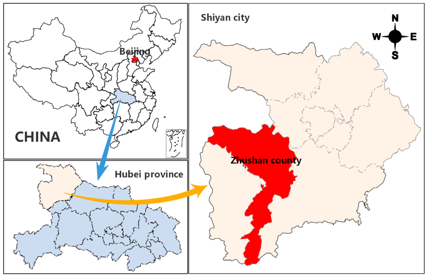
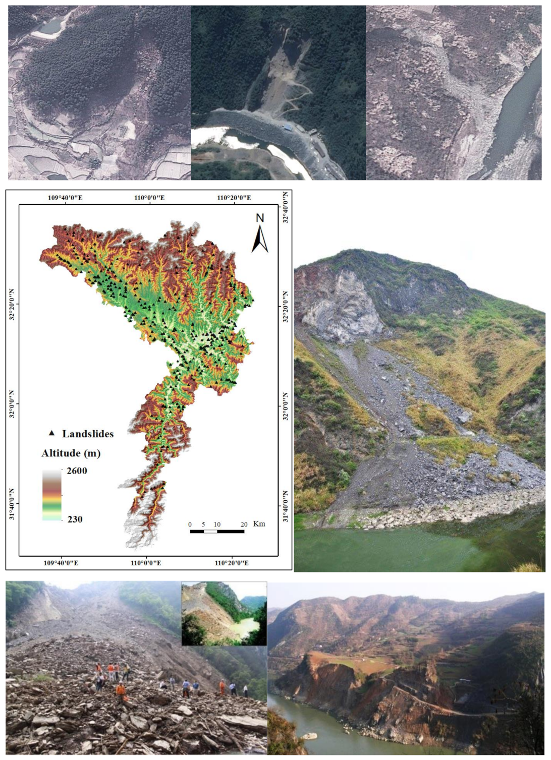
3.1. Description of Study Area

Zhushan County is located in the northwest of Hubei Province of China. It encompasses a total area of 3587.8 km² between the coordinates 109°32′ E and 110°25′ E longitude and 31°30′ N to 32°37′ N latitude Figure 1. The region has a subtropical monsoon climate with abundant rainfall and four distinct seasons. There are a total of 646 rivers, with a river network density of 0.76 km/km². The major geomorphic types are mountainous, hills, rift basins, and valley terraces. The study area includes seven geological age units, which are Sinian, Cambrian, Ordovician, Silurian, Cretaceous, Tertiary, and Quaternary formations. The main lithology of these formations is magmatic, clastic, and carbonate rocks. The Quaternary covers are mainly distributed in the northern and northeastern parts of the study region.

3.2. Landslide Inventory

The geological conditions of Zhushan County are complex, the terrain is undulating, and the distribution density of landslides is high. Based on the long-term field investigation and historical data provided by the Geological Environmental Center of Hubei Province, this study locates 373 landslides.

The landslide inventory data set consists of 373 landslides, which are denoted as black triangles Figure 2. After using the “feature to raster” function of ArcGIS software, the landslide inventory map was converted into raster data with a grid size of 50 m × 50 m. These landslides cover 1010 grid cells on the 1:50,000 DEM map of the study area.

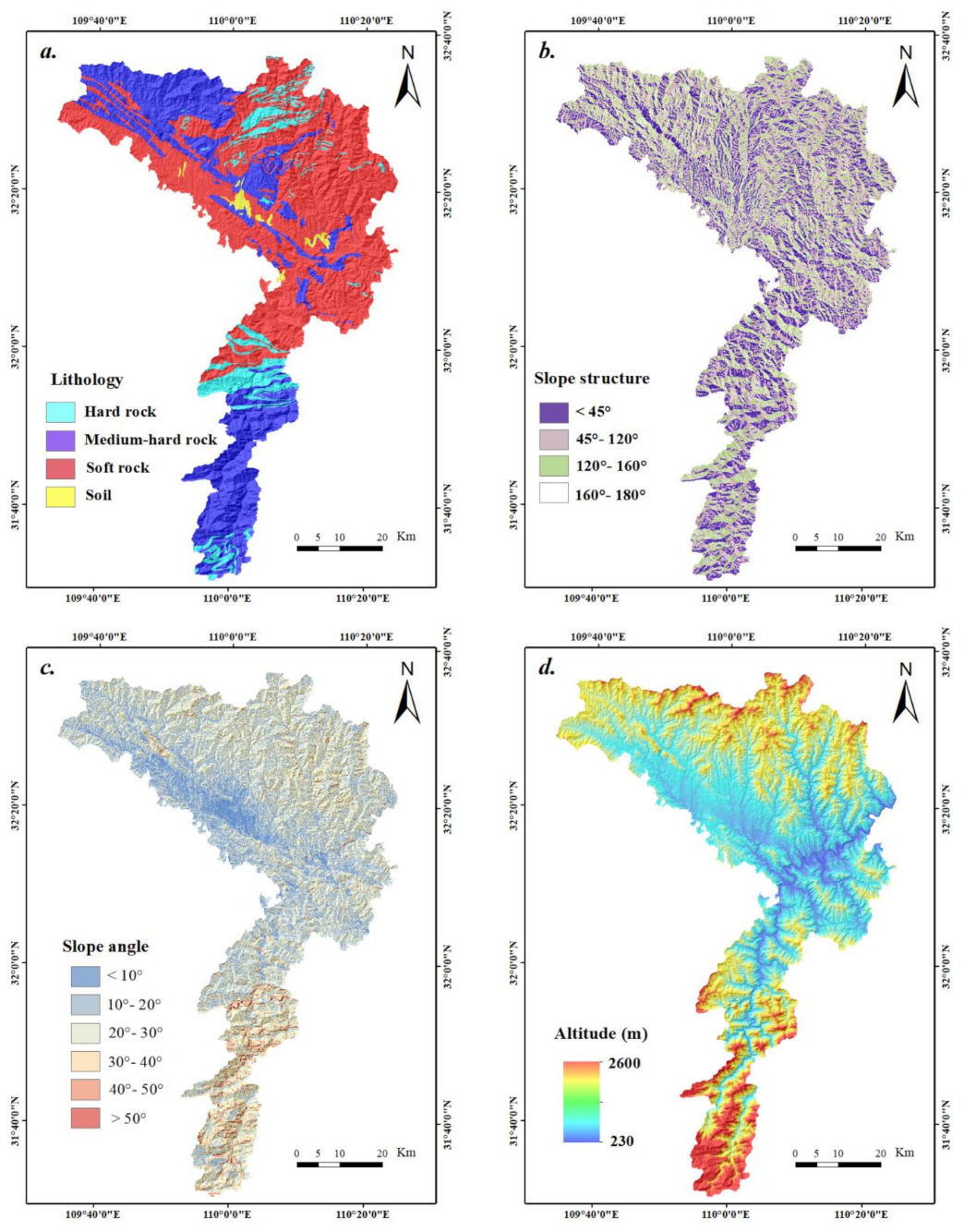
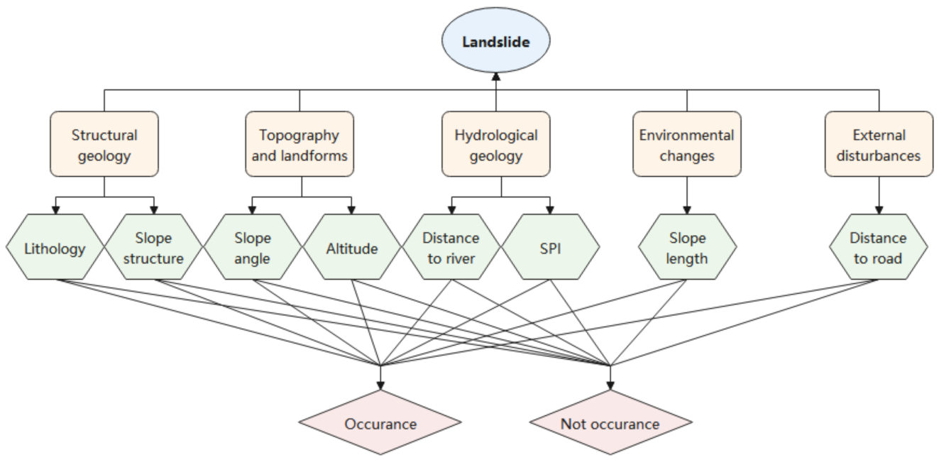
3.3. Conditioning Factors

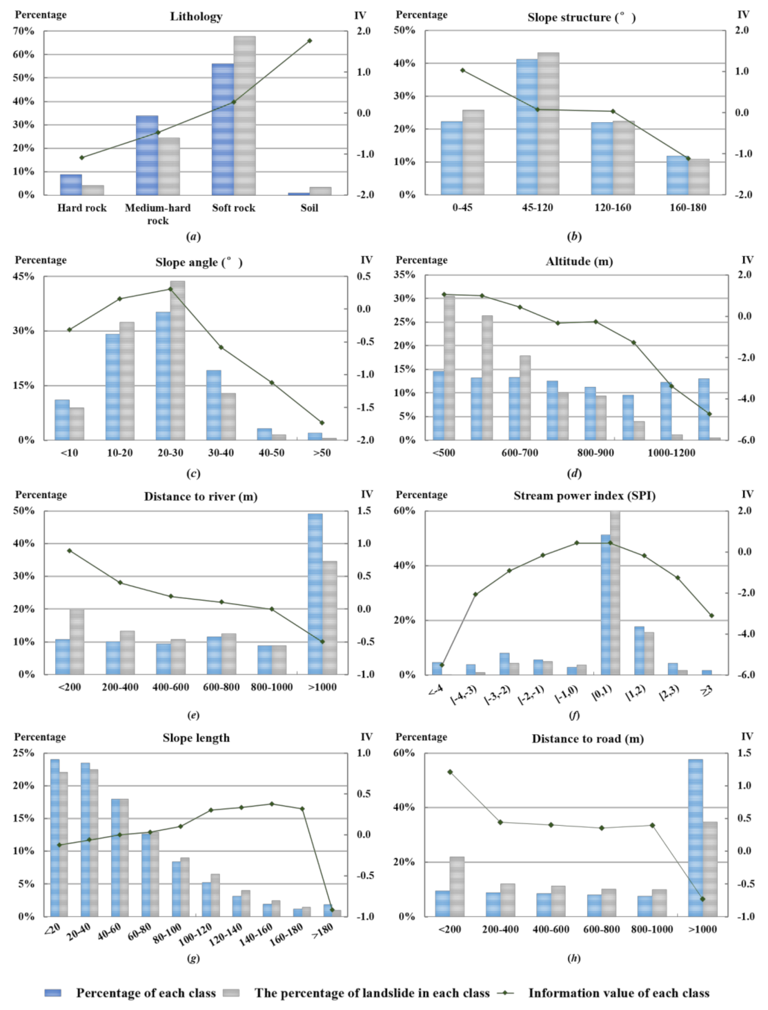
Landslide CFs are essential in LSM [19,57]. Due to the diversity of regional geological backgrounds, there is no universal criterion for conditional factor selection [6,9]. The occurrence of landslides is the result of multiple factors, mainly divided into two types: external inducing factors and intrinsic background factors. The former includes human engineering activities, rainfall, earthquakes, etc. The latter includes topography, geological structure, lithology, etc. Based on the literature, data availability, and our experience, we selected 8 CFs: lithology, slope structure, slope angle, altitude, distance to river, stream power index (SPI), slope length, distance to road.

In order to show the relationship between each CF and the occurrence of landslide, three parameters are given in the form of polyline-histogram, respectively: (1) the percentage of each class of each CF, i.e., $t_{im}=T_{im}/T$; (2) the percentage of landslides in each class of each CF, i.e., $a_{im}=L_{im}/L$; (3) the IV of each class of each CF I_i. See Section 2.2 for specific calculations.

3.4. Lithology

Due to the difference in material strength, slopes with different lithologies have different potentials to become landslides [36]. In this study, considering both mechanical properties and structural integrity of rock and soil mass, the main lithology was reclassified into four types, which are hardest rock, medium-hard rock, soft rock, and soil Figure 3a. The histogram in Figure 4a shows that the soft rock group in the region has the widest distribution range, accounting for 56.17% of the total number of grid cells, and the soil has the smallest distribution range, accounting for only 1.02%. However, from the IV curve, the landslide density in the soil group is the highest, with an IV of 1.76. Meanwhile, the hardest rock group has the lowest IV of −1.09.

3.5. Slope Structure

Slope structure is an important property describing the type of slope and an important indicator of slope stability. It reflects the positional relationship between rock layers and the empty surface of the slope. Slope structure can usually be divided into forward slope, diagonal slope, cross slope, and reverse slope. Different slope structure types have great differences in the development characteristics and degree of landslides. For example, the forward slope is prone to large-scale landslides, controlled by the lithological interface and weak interlayer. Based on the raster calculation function of ArcGIS, this paper uses the angle between the slope aspect and the rock layer inclination (range 0–180°) to characterize the slope structure of the study area [58] and divide the slope structure into 4 types according to the calculation results: 0–45°, 45–120°, 120–160°, and 160–180°, as shown in Figure 3b.

The bar chart in Figure 4b shows that the slope structure of 45–120° has the widest distribution range (43.27%). This is because, in the study area, most of the landslides are cross slopes; the slope structure of 160–180° has the smallest distribution range (10.98%). According to the IV curve, 0–45° is a forward slope, and this range has the maximum IV of 1.03, which is consistent with the conclusion that the forward slope is more prone to landslide.

3.6. Slope Angle

A large number of statistics have shown that the slope angle is closely related to landslide activity [59,60,61,62]. For this reason, it has been considered an important CF in LSM [24,36,53,63,64,65]. In this area, the slope angles are divided into 6 classes, as shown in Figure 3c.

The histogram in Figure 4c shows that slopes with slope angles of 20–30° have the widest distribution range (35.27%). The number of landslides that fall in this class is also the largest (43.66%). The area with a slope angle greater than 50° accounts for the smallest percentage of total area (1.98%), as well as the smallest percentage of existing landslide (0.59%). In addition, according to the IV curve, in the study area, with increasing slope angle, the IV of each class increases first and then decreases, reaching the maximum in the 20–30° class.

3.7. Altitude

Much literature selects the altitude as the CF of landslide [11,12,33,54,66]. It is related to other geological and landform processes, such as weathering erosion, accumulation of debris, and slope deformation, etc. The altitudes in the considered study region range from 230 m to 2600 m (Figure 3d). To facilitate summary, the altitudes are divided into 10 classes, as shown in Figure 4d.

The histogram in Figure 4d shows that the number of grid cells in each class has small differences. The largest number of landslides developed in the section with an altitude of <500 m, accounting for 30.50% of the number of landslides. Besides, the IV of each class decreases with the increase of altitude.

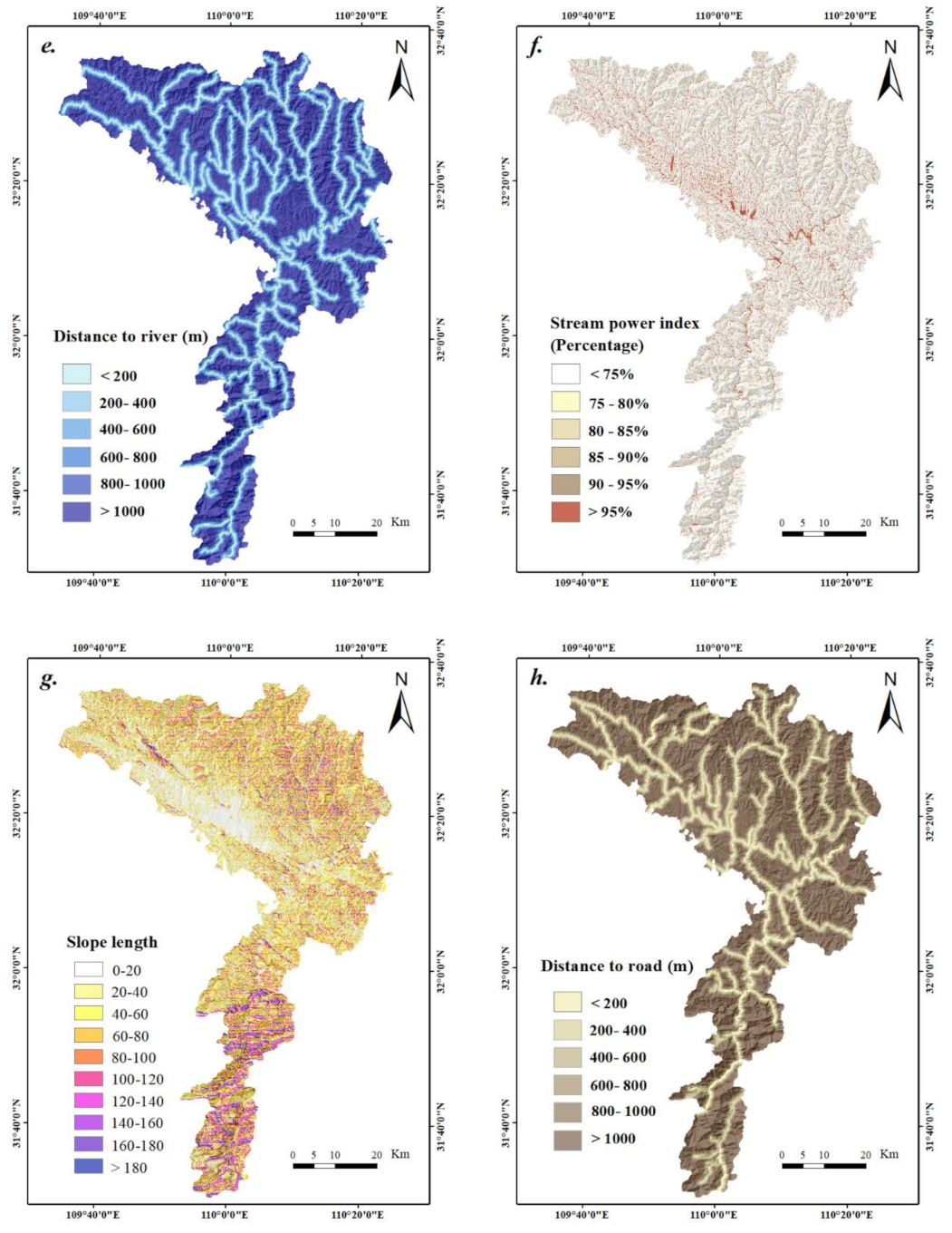
3.8. Distance to River

The water system in the study area mainly includes rivers, seasonal streams, and gullies with low terrain. The distance to river can partially reflect the hydrological environment of the slope, and its significance in landslide occurrence is widely recognized [36,40,43,63,66,67,68]. According to the hydrogeological map of Zhushan County, the distance to river was obtained and divided into 6 classes (Figure 3e).

The histogram in Figure 4e shows that the number of grid cells in the range of >1000 m is the largest (49.19%), and the remaining classes have small differences. The information value curve shows an obvious decreasing trend, indicating that the development of landslide is negatively correlated with the distance to river in Zhushan County. When the distance is less than 200 m, the information value reaches the maximum of 0.89, while when the distance is greater than 1000 m, the information value reaches the minimum of −0.51.

3.9. Stream Power Index (SPI)

The SPI is used to characterize potential erosive power associated with flowing stream [6,69]. It considers the slope geometry as well as the landscape at a given point. Many studies on LSM have noticed the impact of SPI [33,40,70]. It can be calculated by Equation (8) [39]:

$$SPI=A\ast \tan \beta$$

(8)

where A (m²) is the specific catchment area and β (°) is the local slope gradient [39]. The distribution of SPI is shown in Figure 3f.

The histogram in Figure 4f shows that the class with the SPI value [0,1) accounts for the largest percentage of the total grid cells (51.24%), as well as the largest percentage of the landslide grid cells (68.47%), thus owning the maximum information value of 0.42. The information value curve has an approximately normal distribution; with the increase of SPI, the information value first increases and then decreases.

3.10. Slope Length

The slope length is a parameter in the Universal Soil Loss Equation (USLE), which has been taken into account in soil erosions and LSM [71,72,73]. Slope length refers to the distance of uninterrupted overland flow along the slope [73]. Higher erosion rick usually occurs on steeper and longer slopes, and vice versa [74]. The slope length is calculated using Equation (9) [73,75,76]:

$$L_s={\left(\lambda /22.1\right)}^{\beta \left(1+\beta \right)}$$

(9)

where λ is the slope length along the horizontal projection and β is the ratio of rill erosion to interrill erosion. The distribution of slope length is shown in Figure 3g.

The histogram in Figure 4g shows that classes 20–40 (24.06%) and 40–60 (23.51%) have the largest proportions of total grid cells, as well as the largest proportions of landslide grid cells: 34.06% and 28.81%, respectively. According to the information value curve, in the range where slope length is less than 160, as the slope length increases, the information value increases steadily, reaching a maximum value of 0.38 in the class of 140–160. However, when the slope length is greater than 180, the information value drops sharply to a negative value of −0.93.

3.11. Distance to Road

Frequent human engineering activities will exacerbate landslide hazards. A large number of landslides that occurred on embankments or cut slopes confirm this conclusion [77,78]. Therefore, this study, like many others [12,21,54,63,68], regards the distance to road as an important CF in LSM. According to the topographic map of Zhushan County, the distance to road was obtained and divided into 6 classes (Figure 3h).

According to Figure 4h, the number of grid cells with a class >1000 m is far larger than other classes, accounting for 57.72% of the total. The landslides it contains account for 34.75%. In addition, from the IV curve, the development of landslide is negatively correlated with the value of distance to road. When the distance is less than 200 m, the information value reaches the maximum of 1.21, while as the distance is greater than 1000 m, the information value reaches the minimum of −0.73.

4. Landslide Susceptibility Mapping

The LS maps of Zhushan County are respectively produced by the LR model, AHPIV model, and the CLSI model, as shown in Figure 5.

4.1. LSM Using LR Model

In our LR model, eight CFs are taken as independent variables: lithology (x₁), slope structure (x₂), slope angle (x₃), altitude (x₄), distance to river (x₅), SPI (x₆), slope length (x₇), and distance to road (x₈). The CF is normalized in advance. Select all landslide grid cells, 1010 in total, and mark them as 1. Subsequently, 1010 non-landslide grid cells are randomly picked and marked as 0. These 2020 grid cells together form the prediction sample set of the LR model. The data are exported to the statistical analysis software SPSS. The equation of Z is obtained as follows:

$$\begin{array}{c}Z=2.340\times x_1+0.121\times x_2+0.214\times x_3-1.987\times x_4-0.017\times x_5\\ +0.032\times x_6-0.406\times x_7-3.340\times x_8+1.499\end{array}$$

(10)

Subsequently, based on the raster calculation function of ArcGIS, through Equations (1) and (2), the P value of each grid cell is calculated. According to the natural breakpoints method, the LSM results are divided into 5 levels, which are very low (29.84%), low (14.37%), moderate (15.42%), high (29.31%), and very high (11.06%). The LS map obtained by the LR model is shown in Figure 5a.

4.2. LSM Using AHPIV Model

To calculate the I_n of each grid cell using Equation (3), the weight of each factor needs to be determined first, using the AHP method. The key to this method is to build a reasonable hierarchy. According to the landslide investigation data, this article believes that the gestation and development of landslides are controlled by five aspects: structural geology, topography and landforms, hydrological geology, environmental changes, and external disturbances. From these aspects, an evaluation system containing 8 CFs is established, and the hierarchical structure is shown in Figure 6.

According to the hierarchical structure in Figure 6, the first-level and second-level judgment matrices are constructed, as shown in

Table 2. First-level judgment matrix of landslide susceptibility.

First-Level	Structural Geology	Topography and Landforms	Hydrological Geology	Environmental Changes	External Disturbances
Structural geology	1	4	3	2	1
Topography and landforms	1/4	1	2	2	1/3
Hydrogeological geology	1/3	1/2	1	3	1/2
Environmental changes	1/2	1/2	1/3	1	1/2
External disturbances	1	3	2	2	1

and

Table 3. Second-level judgment matrix of landslide susceptibility.

Structural Geology	Lithology	Slope Structure
Lithology	1	3
Slope structure	1/3	1
Topography and Landforms	Slope angle	Altitude
Slope angle	1	2
Altitude	1/2	1
Hydrological Geology	Distance to river	SPI
Distance to river	1	1/2
SPI	2	1

, respectively. Since there is only one secondary CF in the categories of environmental changes and external disturbances, there is no need to construct a second-level judgment matrix.

Through calculation, the CR values of four judgment matrices are respectively 0.09, 0, 0, and 0. All meet the consistency test. The principal eigenvectors of the above matrix are respectively calculated, and the weights of eight CFs are obtained through normalization see

Table 4. Conditioning factor weights determined based on the analytical hierarchy process (AHP) method.

Conditioning Factor	Lithology	Slope Structure	Slope Angle	Altitude	Distance to River	SPI	Slope Length	Distance to Road
	(W1)	(W2)	(W3)	(W4)	(W5)	(W6)	(W7)	(W8)
Weight	0.2512	0.0837	0.0979	0.0490	0.0464	0.0929	0.0968	0.2821

.

In Equation (5), the I_i values correspond to each class for each CF see

Table 5. Relation between landslide occurrence and each class of every conditional factor.

Conditioning Factor	Classes	Total Grid Cells (Tim)	Landslide Grid Cells (Lim)	aim (%)	bim (%)	FR Rim	Ii
Lithology (W1)	Hard rock	124,990	42	4.16	8.85	0.47	−1.09
	Medium-hard rock	480,072	248	24.55	33.97	0.72	−0.47
	Soft rock	794,086	685	67.82	56.17	1.21	0.27
	Soil	14,460	35	3.47	1.02	3.39	1.76
Slope structure (W2)	<45°	155,227	226	22.38	10.97	2.04	1.03
	45–120°	582,184	437	43.27	41.18	1.05	0.07
	120–160°	311,450	227	22.48	22.03	1.02	0.03
	160–180°	364,747	120	11.88	25.81	0.46	−1.12
Slope angle (W3)	<10°	156,748	90	8.91	11.09	0.80	−0.32
	10–20°	412,342	328	32.48	29.17	1.11	0.15
	20–30°	498,615	441	43.66	35.27	1.24	0.31
	30–40°	272,172	130	12.87	19.26	0.67	−0.58
	40–50°	45,756	15	1.49	3.24	0.46	−1.12
	>50°	27,975	6	0.59	1.98	0.30	−1.74
Altitude (W4)	<500	207,120	308	30.50	14.64	2.08	1.06
	500–600	186,742	267	26.44	13.20	2.00	1.00
	600–700	187,723	181	17.92	13.28	1.35	0.43
	700–800	178,184	102	10.10	12.61	0.80	−0.32
	800–900	159,811	95	9.41	11.31	0.83	−0.27
	900–1000	135,327	40	3.96	9.58	0.41	−1.27
	1000–1200	174,245	12	1.19	12.33	0.10	−3.37
	>1200	184,456	5	0.50	13.06	0.04	−4.72
Distance to river (W5)	<200	151,769	201	19.90	10.73	1.85	0.89
	200–400	142,958	135	13.37	10.11	1.32	0.40
	400–600	133,464	109	10.79	9.44	1.14	0.19
	600–800	164,189	126	12.48	11.61	1.07	0.10
	800–1000	124,826	89	8.81	8.83	1.00	0.00
	>1000	696,402	350	34.65	49.27	0.70	−0.51
SPI (W6)	<−4	64,980	1	0.10	4.60	0.02	−5.54
	[−4,−3)	53,501	9	0.89	3.79	0.24	−2.09
	[−3,−2)	114,181	43	4.26	8.08	0.53	−0.92
	[−2,−1)	79,720	50	4.95	5.64	0.88	−0.19
	[−1,0)	39,862	38	3.76	2.82	1.33	0.42
	[0,1)	724,507	692	68.51	51.24	1.34	0.42
	[1,2)	251,458	157	15.54	17.79	0.87	−0.19
	[2,3)	60,901	18	1.78	4.31	0.41	−1.27
	≥3	24,498	2	0.20	1.73	0.11	−3.13
Slope length (W7)	<20	340,160	223	22.08	24.06	0.92	−0.12
	20–40	332,350	228	22.57	23.51	0.96	−0.06
	40–60	254,211	182	18.02	17.98	1.00	0.00
	60–80	178,444	130	12.87	12.62	1.02	0.03
	80–100	118,495	91	9.01	8.38	1.07	0.10
	100–120	74,451	66	6.53	5.27	1.24	0.31
	120–140	44,743	40	3.96	3.16	1.25	0.32
	140–160	27,200	25	2.48	1.92	1.29	0.36
	160–180	16,913	15	1.49	1.20	1.24	0.31
	>180	26,641	10	0.99	1.89	0.53	−0.93
Distance to road (W8)	<200	133,540	221	21.88	9.44	2.32	1.21
	200–400	125,709	122	12.08	8.89	1.36	0.44
	400–600	119,462	113	11.19	8.45	1.32	0.40
	600–800	112,835	103	10.20	7.98	1.28	0.35
	800–1000	106,124	100	9.90	7.51	1.32	0.40
	>1000	815,938	351	34.75	57.74	0.60	−0.73

. Subsequently, based on the raster calculation function of ArcGIS, through Equation (3), the distribution range of I_n in Zhushan County is calculated. By the natural breakpoints method, the LSM results are divided into 5 levels, which are very low (20.76%), low (30.26%), moderate (26.37%), high (18.74%), and very high (3.88%). The LS map obtained by the AHPIV model is shown in Figure 5b.

4.3. LSM Using the CLSI Model

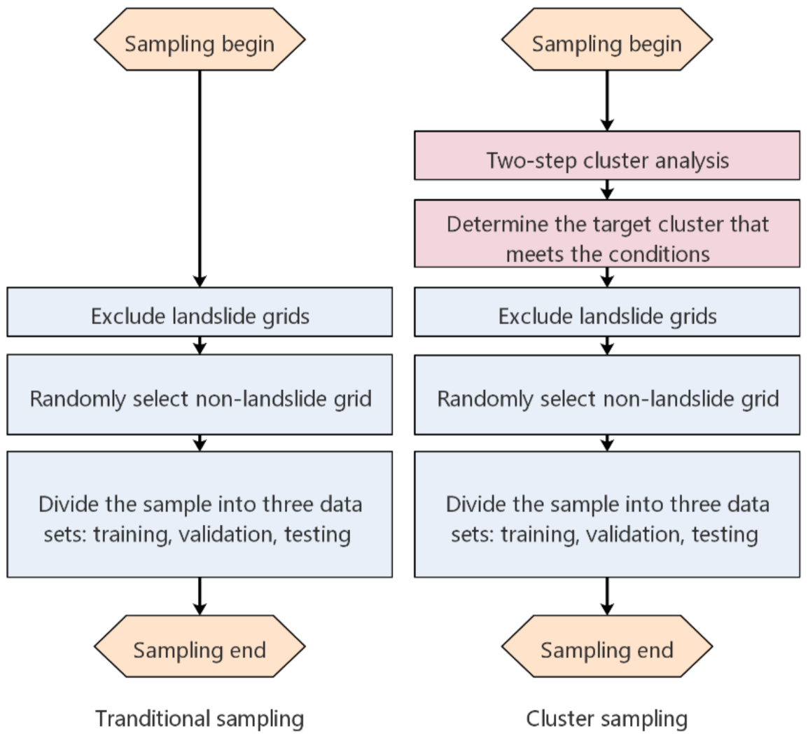
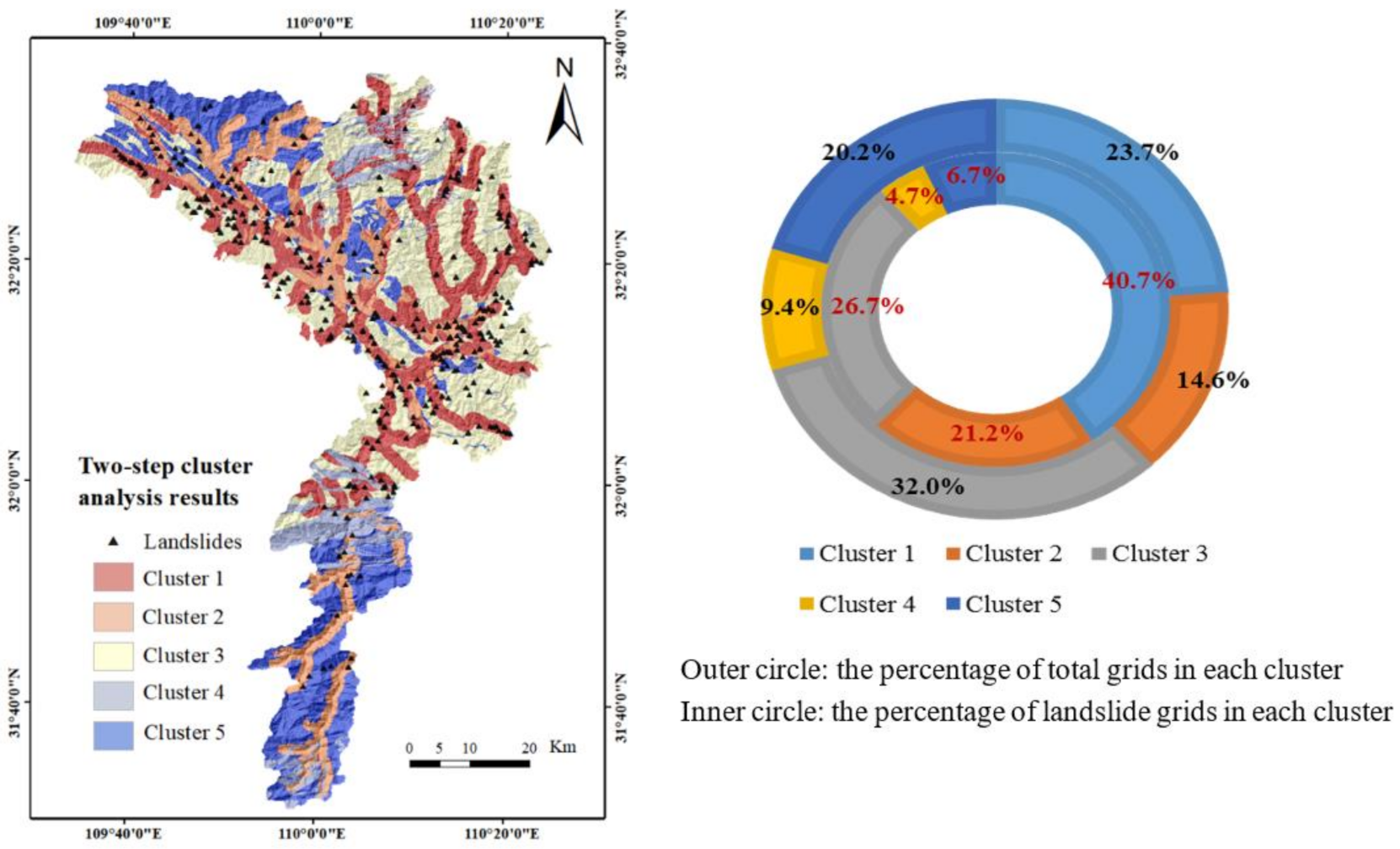
4.3.1. Non-Landslide Area Selection

Before the BPNN procedure, the two-step cluster analysis (TSCA) was used for sample preprocessing. In order to determine a dataset that can better characterize the geological environmental conditions of non-landslide, Figure 7 shows the difference between the sampling process in this study and the traditional sampling process.

Due to their close relationship with the landslide occurrence, these eight CFs were also used as evaluation indicators for TSCA. Data normalization is required before analysis. The study region is divided into 5 clusters, and the results are shown in Figure 8.

The distribution of the clusters in Figure 8 shows that (1) only Clusters 1 and 2 have an obvious band-like distribution trend, and the rest are distributed in the form of scattered areas; (2) the clustering result is controlled by multiple evaluation factors such as lithology, distance to river, etc.; and (3) the outer circle shows relatively small differences of total grid cells in each cluster, meanwhile, the inner circle shows big differences of landslide grid cells in each cluster.

The following conditions are used to filter the target clusters for non-landslide grid cells sampling. Among them, condition 1 refers to [5].

$$\mathrm{Condition}-1: C_1=\frac{N_c}{N_t}<0.1$$

(11)

$$\mathrm{Condition}-2: C_2=\min \left(\frac{P_c}{P_t}\right)$$

(12)

where $N_c$ denotes the number of landslide grid cells for each cluster, $N_t$ denotes the number of landslide grid cells in the whole area ($N_t=1010$), $P_c$ equals to the number of landslide grid cells in each cluster divided by the number of total grid cells in each cluster, and $P_t$ denotes the percentage of landslides in Zhushan County ($P_t=1010/\mathrm{1,413,608}$).

According to the clustering results and screening conditions see

Table 6. Subdivision of the study area into five clusters by the two-step cluster analysis.

Cluster Number	1	2	3	4	5	Total in the Study Area
Number of landslide grid cells	411	214	270	47	68	1010
Number of non-landslide grid cells	334,504	206,144	452,506	133,266	286,178	1,412,598
Total number of grid cells	334,915	206,358	452,776	133,313	286,246	1,413,608
Sampling condition 1 ($N_c/N_t$)	0.41	0.21	0.27	0.05	0.07
Sampling condition 2 ($P_c/P_t$)	1.72	1.45	0.83	0.49	0.33

, the clusters that meet condition 1 include Clusters 4 and 5. Based on the second condition, the cluster with the minimum C₂ value is the most suitable cluster for random sampling of non-landslide, i.e., Cluster 5.

4.3.2. Weight Determination for Each Factor

In this study, a three-layered BPNN model was applied for weight determination using the MATLAB software package. The input nodes are the CFs, the number is 8 (N_i = 8). The output node is the value of LSI (N_o = 1). For the number of hidden layer nodes (N_h), the upper limit is (2N_i + 1) [79], and the lower limit is (N_i + N_o)/2 [80]; thus the best range of hidden layer nodes is 5 ≤ N_h ≤ 17. After comparing 5, 10, 12, 15, and 17 as possible hidden layer nodes, 15 nodes were identified as the best. Based on this, a BPNN model with a structure of 8-15-1 is established.

According to the literature [81], the training sample size (N_sample) for the three-layered BPNN model can be determined by Equation (13).

$$\frac{W}{\epsilon }\le N_{sample}\le \frac{W}{\epsilon }·\log \frac{N}{\epsilon }$$

(13)

where N denotes the total number of nodes, W denotes the total number of weights, and ε denotes the accuracy parameter. In this study, assume the model has an accuracy level of 90%, and thus the ε equals to 0.1 and the range of training sample number is [1350, 3213]. Therefore, 2510 grid cells were selected, including all landslide grid cells (1010) and 1500 non-landslide grid cells (selected from Cluster 5). Among them, 80% is used for model training, and 20% is used for model validation. For transfer functions and other parameters [82], please see

Table 7. Parameter settings in back-propagation neural network (BPNN) analysis.

Table 1		Training Method	Epochs	Learning Rate	RMSE Goal
Hidden (f1)	Output (f2)
Logsig	Purelin	LM	1000	0.01	0.01

Logsig: log-sigmoid transfer function; Purelin: linear transfer function; LM: Levenberg–Marquardt algorithm, which has good generalization ability and has the capability of providing good predictions [82].

.

In order to make the results more rigorous, the calculation was repeated 10 times to achieve the average value see

Table 8. Weight of each factor determined by BPNN.

Conditioning Factor	1	2	3	4	5	6	7	8	9	10	COV	Mean	Weight
Lithology	1.653	1.655	1.661	1.687	1.618	1.646	1.871	1.875	1.715	1.744	0.0921	1.71	2.35
Slope structure	0.728	0.731	0.749	0.762	0.777	0.785	0.829	0.838	0.912	0.946	0.0749	0.81	1.10
Slope angle	1.110	1.018	1.087	1.119	1.121	1.130	1.246	1.264	1.297	1.198	0.0885	1.16	1.59
Altitude	0.774	0.778	0.854	0.895	0.928	0.939	0.948	0.977	0.983	0.998	0.0814	0.91	1.24
Distance to river	0.800	0.803	0.770	0.793	0.799	0.839	0.853	0.854	0.896	0.900	0.0446	0.83	1.14
SPI	0.650	0.683	0.688	0.695	0.719	0.740	0.749	0.749	0.805	0.826	0.0552	0.73	1.00
Slope length	0.647	0.662	0.678	0.709	0.723	0.731	0.782	0.798	0.813	0.826	0.0645	0.74	1.01
Distance to road	1.391	1.409	1.412	1.488	1.409	1.538	1.438	1.445	1.460	1.483	0.0455	1.45	1.98

. The covariance values (COVs) indicated that the difference between the 10 calculations is small, and the overall result is reasonable and reliable. In Table 7, the mean values represent the calculated average weights of CFs, and the last column is the normalized weight of each CF. The SPI has the minimum weight while the lithology has the maximum weight. The results show that lithology has the greatest impact on the occurrence of landslides, which is very consistent with the actual survey situation. Moreover, the weight value of distance to road is second only to lithology. In the field investigation, part of the landslides in the study area were found distributed along the roads. The slope angle also has a greater impact on landslide occurrence, which is consistent with the situation shown in the CF analysis. Factors with a relatively small degree of influence are SPI and slope length.

4.3.3. Landslide Susceptibility Map

After the weights are determined, the FR of each class of the 8 CFs is obtained according to Equation (7), as shown in Table 5.

After obtaining the weights and the frequency ratios, the LSI value of each grid cell was calculated according to Equation (6). Based on the natural breakpoints method, the LSM results are divided into 5 levels, which are very low (19.49%), low (20.42%), moderate (23.29%), high (26.91%), and very high (9.89%). The LS map obtained by the CLSI model is shown in Figure 5c.

5. Validation and Analysis

The performance of the LSM model can be evaluated from two aspects. First, whether the model can accurately predict the nonlinear relationship between CFs and the occurrence of landslides based on the available data, i.e., explore the rules and use this to evaluate the landslide susceptibility within unknown areas. The higher the accuracy of the evaluation, the better the model performance. For practical application, the second criterion is the classification ability. The greater the difference between each zone, the higher the classification ability. Considering these two aspects, we did the following verification work.

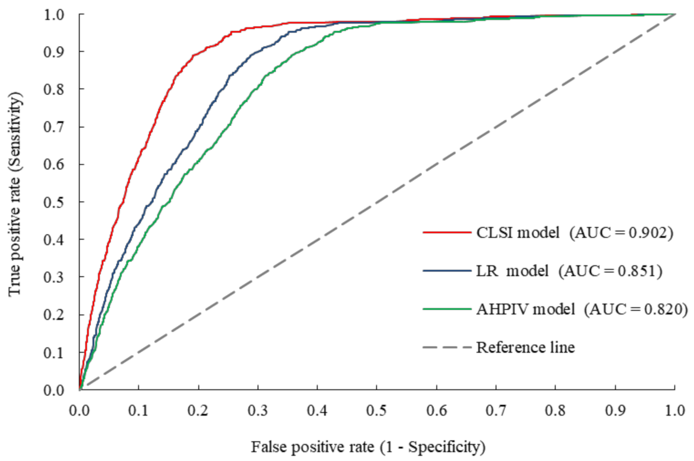
5.1. Validation Based on AUC Accuracy

Regarding the first aspect, the accuracy of the LSM results must be verified. For this purpose, the receiver operating characteristic (ROC) curve and area under the curve (AUC), which have been widely used in previous studies [3,19,42,83], were applied in this study. The ROC curve reflects the corrections between the “Sensitivity” (Equation (14)) and “1-Specificity” (Equation (15)) [6], which are:

$$Sensitivity=\frac{TP}{TP+FN}$$

(14)

$$1-Specificity=\frac{TN}{FP+TN}$$

(15)

where TP is the true positive rate, FN is false negative rate, TN is true negative rate, and FP is false positive rate. The range of the AUC value is [0.5, 1], which reflects the overall accuracy of the prediction. The larger the value, the higher the model accuracy. Note that “false positive” means that a stable area is misjudged as a landslide-prone area. On the contrary, “false negative” refers to the situation that the landslide-prone area is misjudged as a stable area.

In this study, a total of 71,640 grid cells were used to complete three ROC curves using SPSS software. All landslide grid cells were used to form a positive data set, and 5% of non-landslide grid cells that had not participated in the previous calculations were randomly selected to form a negative data set. The result is shown in Figure 9. The prediction accuracy of the three models exceeds 80%, indicating a relatively good prediction performance. This laterally confirms the rationality of the selected CFs.

Figure 9 also suggests the CLSI model has the highest AUC value of 0.902, followed by the LR model (0.851) and the AHPIV model (0.820). The bias in determining the weights by the AHP method greatly reduces the accuracy of the AHPIV model. The CLSI model adopts the more objective and rational BPNN in determining the weights, thus leading to a better result. Benefiting from the rich historical survey data and the approximately linear relationship between some CFs and the occurrence of landslides (e.g., distance to river, distance to road), the performance of the LR model is also remarkable.

5.2. Validation Based on Seed Cell Area Index

Regarding the second aspect, the classification ability of the three LSM models must be verified. A good classifier produces a large difference between the divided zones. In this study, the seed cell area index (SCAI) [84] was used to quantify the difference. The landslide grid cell is called a “seed cell”, and the SCAI can be obtained by

$$SCAI=\frac{P_{area}}{P_{seed}}$$

(16)

where P_area suggests the percentage of grid cells in each susceptibility zone to total grid cells in the whole area and P_seed suggests the percentage of landslide grid cells in each susceptibility zone to grid cells of all landslides. The SCAI is a dimensionless parameter. Generally, the high-proneness area should have a lower SCAI value, and vice versa. A greater difference in SCAIs between the high-proneness area and the low-proneness area indicates a better performance of the model.

The SCAI values are calculated and shown in

Table 9. Comparison results of seed cell area index (SCAI).

LSM Model	Class	Number of Total Grid Cells	Area (%)	Number of Landslide Grid Cells	Seed (%)	SCAI	D-Value
LR model	Very high	156,409	11.06%	325	32.18%	0.34
							0.31
	High	414,279	29.31%	455	45.05%	0.65
							0.62
	Moderate	217,990	15.42%	123	12.18%	1.27
							1.24
	Low	203,160	14.37%	58	5.74%	2.50
							3.65
	Very low	421,770	29.84%	49	4.85%	6.15
AHPIV model	Very high	54,789	3.88%	153	15.15%	0.26
							0.24
	High	264,874	18.74%	385	38.12%	0.49
							0.36
	Moderate	372,714	26.37%	313	30.99%	0.85
							1.30
	Low	427,744	30.26%	142	14.06%	2.15
							10.18
	Very low	293,487	20.76%	17	1.68%	12.33
CLSI model	Very high	139,830	9.89%	306	30.30%	0.33
							0.32
	High	380,421	26.91%	418	41.39%	0.65
							0.47
	Moderate	329,194	23.29%	210	20.79%	1.12
							2.32
	Low	288,611	20.42%	60	5.94%	3.44
							8.87
	Very low	275,552	19.49%	16	1.58%	12.30

. From very low area to very high area, the SCAI values present a decreasing trend for the three models. These results also demonstrate the rationality of the three models. In addition, the SCAI differences between the very low and very high areas for the AHPIV and CLSI model are 12.08 and 11.98, respectively, and they both are far greater than that of the LR model (5.81). This is because the LR model has a large number of landslide grid cells in the very low area, which directly leads to poor interval division. The last column in Table 9 lists the difference value (D-value) of SCAI between adjacent zones. It can be seen that all the minimum D-values fall into the AHPIV and LR model, while there are two maximum D-values that fall into the CLSI model. This result indicates that, in addition to the accuracy, the CLSI model performs the best in classification ability. This is to be expected because the CLSI uses the trained BPNN to calculate the weights, and this captures the nonlinear relationship between the CFs and the occurrence of landslides, leading to more objective and scientific LSM results.

5.3. Validation Based on Landslide Points

Verification of the three landslide susceptibility maps was also performed based on existing landslide points. After LSM, the 373 existing landslides were marked on three LS maps (Figure 10), most of which are located in the very high and high susceptibility zones. From very low to very high susceptible zone, the number of landslide grid cells increases. The AHPIV model showed the worst performance. The CLSI model and LR model showed a better and similar performance. The LR model has a small value of the line slope between the very low area and the low area, indicating that the LR model has a weak ability to identify the low-proneness area. This is consistent with the results of the SCAI verification. However, the LR model has the largest line slope between the moderate area and high area. The CLSI model has a better resolution ability in identifying the very low area and the very high area, but it is slightly inferior to the LR model in distinguishing the moderate area and the high area. In summary, the LSM results show good consistency with the historical landslides, especially the results of the CLSI and LR model.

6. Discussion and Conclusions

In the past few decades, regional LSM has become a frontier research topic due to its complexity and nonlinear characteristics. A variety of methods have been used to establish the evaluating models. The authors have established a comprehensive landslide susceptibility index model (CLSI) [6], which is an integration of prior knowledge and an objective weighting method. To further verify the superiority and generalizability of this model, Zhushan County was taken as the study region. It is a landslide-prone area in Hubei Province of China. Two representative methods, namely, the LR and the analytic hierarchy process information value (AHPIV) model, were used for comparison. Specifically, LR represents the traditional statistical method, and AHPIV represents an integrated method that combines prior knowledge and subjective weight determination.

The LS maps (Figure 5) generated by the three models were well coincident with each other. Specifically, the very high and high susceptibility areas are located along the roads and rivers within a distance of 200m. In addition, lithology also plays a vital role, especially for the soil distribution area. For example, the weights obtained by both the AHP method and BPNN method are highly correlated with the lithology and the distance to road. Moreover, because there are many shallow landslides in Zhushan County, a slope angle less than 30° significantly contributes to the development of landslides.

On the other hand, the very low and low susceptibility areas are far from the river network and road network. These areas have a strong correlation with altitude, with most landslides distributed in zones with altitudes higher than 800 m. This phenomenon can be explained as follows. First, these areas are less affected by human engineering activities; hence the slope stability is higher. Second, due to the strong denudation in high altitude areas, few Quaternary deposits and strong weathering soft rocks accumulate in this area, which provide little material source for shallow landslides.

Generally, a good LSM model performs well in both result accuracy and susceptibility zone classification. Therefore, the performances of these three LSM models were validated in terms of these two aspects. The ROC curve and the value of SCAI were used as the indicators for these two aspects. The ROC results show that LSM in Zhushan County using the three models is viable, and the CLSI model has the highest AUC value of 0.902, followed by the LR (0.851) and AHPIV (0.820). The validation based on SCAI values indicate that these three models generate reasonable LSM partitions, and the CLSI model has the best classification ability. Subsequently, the existing landslide grid cell accumulation curves were used for further verification. A good agreement was obtained between the LS maps and existing landslides. The CLSI model has a better ability in identifying the very low area and the very high area. Through these comparisons, this study clearly reveals that the robust performance of the CLSI lies in the weight determination, that is, the determined weights by the BPNN successfully captures the nonlinear relationship between the CFs and the occurrence of landslides.

There are some literature regarding the comparison of the LR model and other existing methods in LSM [2,10,36,37,39,46]. Du et al. [34] compared the LR model, IV model, and LRIV model. The success rates were 69.2%, 68.8%, and 81.7%, respectively. The prediction rates were 78.5%, 71.6%, and 84.6%, respectively. This study showed that the performance of the LR model is in the middle position. Akgun [63] compared the LR model, likelihood ratio, and multi-criteria decision analysis. The LR was determined to be the most accurate method compared to the other two. Merghadi et al. [85] did a lot of work to compare the application of machine learning methods including the LR model. They believed that although the AUC value of the LR model is greater than 0.82, it has no accuracy advantage compared to other machine learning methods.

In addition, a few documents discuss the performance of the AHPIV model in landslide susceptibility mapping. Zhang et al. [31] elaborated on the process and prediction performance of the AHPIV model. The AUC value of this model was 0.694 for the prediction rate. Du et al. [8] compared two integrated models (the AHPIV and the LRIV) in LSM. The performances of the methods were also validated and compared using ROC curves. The AUC values obtained using the AHPIV and LRIV methods were 0.884 and 0.906, respectively. Results show that the LRIV method performs better than the AHPIV method. Banerjee et al. [86] also applied the AHPIV method to the field of LSM. The evaluation accuracy analysis result of this model was 85%.

Although scholars are committed to the comparison of different methods, it is hard to reach a consensus. Due to different prior knowledge of each study (i.e., different geological backgrounds, different types of occurrence landslides, and different conditioning factors), it is not possible to make a horizontal comparison. However, is the CLSI model superior to other methods besides the LR and AHPIV model or not? Can the selection of more conditioning factors give better LSM results or not? These problems need to be addressed and solved in our future study.

In summary, the main contributions of this research are (1) the LSM processes using the LR model, the AHPIV model, and the CLSI model was explored and summarized; (2) eight CFs of lithology, slope structure, slope angle, altitude, distance to river, SPI, and distance to road are reasonable CFs for LSM in Zhushan County; (3) reasonable LS maps of Zhushan County were produced in ArcGIS software; (4) the CLSI model was found to be more appropriate for LSM than the LR model and AHPIV model, in terms of result accuracy and classification ability; and (5) the CLSI model can be used as a robust predictor for the County-level area.

References

1. Nadim, F.; Kjekstad, O.; Peduzzi, P.; Herold, C.; Jaedicke, C. Global landslide and avalanche hotspots. Landslides 2006, 3, 159–173. [Google Scholar] [CrossRef]
2. Nhu, V.-H.; Mohammadi, A.; Shahabi, H.; Ahmad, B.B.; Al-Ansari, N.; Shirzadi, A.; Geertsema, M.; Kress, V.R.R.; Karimzadeh, S.; Kamran, K.; et al. Landslide Detection and Susceptibility Modeling on Cameron Highlands (Malaysia): A Comparison between Random Forest, Logistic Regression and Logistic Model Tree Algorithms. Forests 2020, 11, 830. [Google Scholar] [CrossRef]
3. Arabameri, A.; Saha, S.; Roy, J.; Chen, W.; Blaschke, T.; Bui, D.T. Landslide Susceptibility Evaluation and Management Using Different Machine Learning Methods in The Gallicash River Watershed, Iran. Remote Sens. 2020, 12, 475. [Google Scholar] [CrossRef] [Green Version]
4. Maurizio, L.; Maria, D. A multi temporal kernel density estimation approach for new triggered landslides forecasting and susceptibility assessment. Disaster Adv. 2012, 5, 100–108. [Google Scholar]
5. Melchiorre, C.; Matteucci, M.; Azzoni, A.; Zanchi, A. Artificial neural networks and cluster analysis in landslide susceptibility zonation. Geomorphology 2008, 94, 379–400. [Google Scholar] [CrossRef]
6. Tang, R.; Kulatilake, P.H.S.W.; Yan, E.-C.; Cai, J.-S. Evaluating landslide susceptibility based on cluster analysis, probabilistic methods, and artificial neural networks. Bull. Int. Assoc. Eng. Geol. 2020, 79, 2235–2254. [Google Scholar] [CrossRef]
7. Tang, R. Research on Stability Evaluation of Individual Colluvial Landslides and Regional Landslide Susceptibility Analysis; China University of Geoscience: Wuhan, China, 2017; p. 170. [Google Scholar]
8. Du, G.; Zhang, Y.; Yang, Z.; Guo, C.; Yao, X.; Sun, D. Landslide susceptibility mapping in the region of eastern Himalayan syntaxis, Tibetan Plateau, China: A comparison between analytical hierarchy process information value and logistic regression-information value methods. Bull. Int. Assoc. Eng. Geol. 2019, 78, 4201–4215. [Google Scholar] [CrossRef]
9. Ayalew, L.; Yamagishi, H.; Marui, H.; Kanno, T. Landslides in Sado Island of Japan: Part II. GIS-based susceptibility mapping with comparisons of results from two methods and verifications. Eng. Geol. 2005, 81, 432–445. [Google Scholar] [CrossRef]
10. Wang, L.-J.; Guo, M.; Sawada, K.; Lin, J.; Zhang, J. A comparative study of landslide susceptibility maps using logistic regression, frequency ratio, decision tree, weights of evidence and artificial neural network. Geosci. J. 2016, 20, 117–136. [Google Scholar] [CrossRef]
11. Pourghasemi, H.R.; Pradhan, B.; Gokceoglu, C. Application of fuzzy logic and analytical hierarchy process (AHP) to landslide susceptibility mapping at Haraz watershed, Iran. Nat. Hazards 2012, 63, 965–996. [Google Scholar] [CrossRef]
12. Myronidis, D.; Papageorgiou, C.; Theophanous, S. Landslide susceptibility mapping based on landslide history and analytic hierarchy process (AHP). Nat. Hazards 2016, 81, 245–263. [Google Scholar] [CrossRef]
13. Moragues, S.; Lenzano, M.G.; Lanfri, M.; Moreiras, S.; Lannutti, E.; Lenzano, L. Analytic hierarchy process applied to landslide susceptibility mapping of the North Branch of Argentino Lake, Argentina. Nat. Hazards 2021, 105, 915–941. [Google Scholar] [CrossRef]
14. Kayastha, P.; Dhital, M.; De Smedt, F. Application of the analytical hierarchy process (AHP) for landslide susceptibility mapping: A case study from the Tinau watershed, west Nepal. Comput. Geosci. 2013, 52, 398–408. [Google Scholar] [CrossRef]
15. Bui, D.T.; Pradhan, B.; Lofman, O.; Revhaug, I.; Dick, O.B. Landslide susceptibility assessment in the Hoa Binh province of Vietnam: A comparison of the Levenberg–Marquardt and Bayesian regularized neural networks. Geomorphology 2012, 171–172, 12–29. [Google Scholar] [CrossRef]
16. Pradhan, B.; Lee, S. Delineation of landslide hazard areas on Penang Island, Malaysia, by using frequency ratio, logistic regression, and artificial neural network models. Environ. Earth Sci. 2010, 60, 1037–1054. [Google Scholar] [CrossRef]
17. Poudyal, C.P.; Chang, C.; Oh, H.-J.; Lee, S. Landslide susceptibility maps comparing frequency ratio and artificial neural networks: A case study from the Nepal Himalaya. Environ. Earth Sci. 2010, 61, 1049–1064. [Google Scholar] [CrossRef]
18. Lee, S.; Sambath, T. Landslide susceptibility mapping in the Damrei Romel area, Cambodia using frequency ratio and logistic regression models. Environ. Earth Sci. 2006, 50, 847–855. [Google Scholar] [CrossRef]
19. Aditian, A.; Kubota, T.; Shinohara, Y. Comparison of GIS-based landslide susceptibility models using frequency ratio, logistic regression, and artificial neural network in a tertiary region of Ambon, Indonesia. Geomorphology 2018, 318, 101–111. [Google Scholar] [CrossRef]
20. Yao, X.; Tham, L.; Dai, F. Landslide susceptibility mapping based on Support Vector Machine: A case study on natural slopes of Hong Kong, China. Geomorphology 2008, 101, 572–582. [Google Scholar] [CrossRef]
21. Wang, J.; Yin, K.; Xiao, L. Landslide Susceptibility Assessment Based on Gis and Weighted Information Valuea: A Case Study of Wanzhou District, Three Gorges Reservoir. Chin. J. Rock Mech. Eng. 2014, 33, 797–808. [Google Scholar]
22. Lee, C.F.; Li, J.; Xu, Z.W.; Dai, F.C. Assessment of landslide susceptibility on the natural terrain of Lantau Island, Hong Kong. Environ. Earth Sci. 2001, 40, 381–391. [Google Scholar] [CrossRef]
23. Gorsevski, P.V.; Gessler, P.E.; Foltz, R.B.; Elliot, W.J. Spatial Prediction of Landslide Hazard Using Logistic Regression and ROC Analysis. Trans. GIS 2006, 10, 395–415. [Google Scholar] [CrossRef]
24. Catani, F.; Casagli, N.; Ermini, L.; Righini, G.; Menduni, G. Landslide hazard and risk mapping at catchment scale in the Arno River basin. Landslides 2005, 2, 329–342. [Google Scholar] [CrossRef]
25. Marjanović, M.; Kovačević, M.; Bajat, B.; Voženílek, V. Landslide susceptibility assessment using SVM machine learning algorithm. Eng. Geol. 2011, 123, 225–234. [Google Scholar] [CrossRef]
26. Huang, F.; Yin, K.; Huang, J.; Gui, L.; Wang, P. Landslide susceptibility mapping based on self-organizing-map network and extreme learning machine. Eng. Geol. 2017, 223, 11–22. [Google Scholar] [CrossRef]
27. Vasu, N.N.; Lee, S.-R. A hybrid feature selection algorithm integrating an extreme learning machine for landslide susceptibility modeling of Mt. Woomyeon, South Korea. Geomorphology 2016, 263, 50–70. [Google Scholar] [CrossRef]
28. Liu, C.-N.; Wu, C.-C. Mapping susceptibility of rainfall-triggered shallow landslides using a probabilistic approach. Environ. Earth Sci. 2008, 55, 907–915. [Google Scholar] [CrossRef]
29. Wang, W.; He, Z.; Han, Z.; Li, Y.; Dou, J.; Huang, J. Mapping the susceptibility to landslides based on the deep belief network: A case study in Sichuan Province, China. Nat. Hazards 2020, 103, 3239–3261. [Google Scholar] [CrossRef]
30. Zhou, S.; Chen, G.; Fang, L.; Nie, Y. GIS-Based Integration of Subjective and Objective Weighting Methods for Regional Landslides Susceptibility Mapping. Sustainability 2016, 8, 334. [Google Scholar] [CrossRef] [Green Version]
31. Zhang, G.; Cai, Y.; Zheng, Z.; Zhen, J.; Liu, Y.; Huang, K. Integration of the Statistical Index Method and the Analytic Hierarchy Process technique for the assessment of landslide susceptibility in Huizhou, China. Catena 2016, 142, 233–244. [Google Scholar] [CrossRef]
32. Umar, Z.; Pradhan, B.; Ahmad, A.; Jebur, M.N.; Tehrany, M.S. Earthquake induced landslide susceptibility mapping using an integrated ensemble frequency ratio and logistic regression models in West Sumatera Province, Indonesia. Catena 2014, 118, 124–135. [Google Scholar] [CrossRef]
33. Youssef, A.M.; Pradhan, B.; Jebur, M.N.; El-Harbi, H.M. Landslide susceptibility mapping using ensemble bivariate and multivariate statistical models in Fayfa area, Saudi Arabia. Environ. Earth Sci. 2015, 73, 3745–3761. [Google Scholar] [CrossRef]
34. Du, G.-L.; Zhang, Y.-S.; Iqbal, J.; Yang, Z.-H.; Yao, X. Landslide susceptibility mapping using an integrated model of information value method and logistic regression in the Bailongjiang watershed, Gansu Province, China. J. Mt. Sci. 2017, 14, 249–268. [Google Scholar] [CrossRef]
35. Fang, Z.; Wang, Y.; Peng, L.; Hong, H. Integration of convolutional neural network and conventional machine learning classifiers for landslide susceptibility mapping. Comput. Geosci. 2020, 139, 104470. [Google Scholar] [CrossRef]
36. Kanungo, D.; Arora, M.; Sarkar, S.; Gupta, R. A comparative study of conventional, ANN black box, fuzzy and combined neural and fuzzy weighting procedures for landslide susceptibility zonation in Darjeeling Himalayas. Eng. Geol. 2006, 85, 347–366. [Google Scholar] [CrossRef]
37. Chen, T.; Niu, R.; Jia, X. A comparison of information value and logistic regression models in landslide susceptibility mapping by using GIS. Environ. Earth Sci. 2016, 75, 867. [Google Scholar] [CrossRef]
38. Nefeslioglu, H.A.; Gokceoglu, C.; Sonmez, H. An assessment on the use of logistic regression and artificial neural networks with different sampling strategies for the preparation of landslide susceptibility maps. Eng. Geol. 2008, 97, 171–191. [Google Scholar] [CrossRef]
39. Yilmaz, I. Landslide susceptibility mapping using frequency ratio, logistic regression, artificial neural networks and their comparison: A case study from Kat landslides (Tokat—Turkey). Comput. Geosci. 2009, 35, 1125–1138. [Google Scholar] [CrossRef]
40. Pradhan, B. A comparative study on the predictive ability of the decision tree, support vector machine and neuro-fuzzy models in landslide susceptibility mapping using GIS. Comput. Geosci. 2013, 51, 350–365. [Google Scholar] [CrossRef]
41. Bui, D.T.; Tuan, T.A.; Klempe, H.; Pradhan, B.; Revhaug, I. Spatial prediction models for shallow landslide hazards: A comparative assessment of the efficacy of support vector machines, artificial neural networks, kernel logistic regression, and logistic model tree. Landslides 2016, 13, 361–378. [Google Scholar] [CrossRef]
42. Zhang, Y.; Ge, T.; Tian, W.; Liou, Y.-A. Debris Flow Susceptibility Mapping Using Machine-Learning Techniques in Shigatse Area, China. Remote Sens. 2019, 11, 2801. [Google Scholar] [CrossRef] [Green Version]
43. Huang, F.; Cao, Z.; Guo, J.; Jiang, S.-H.; Li, S.; Guo, Z. Comparisons of heuristic, general statistical and machine learning models for landslide susceptibility prediction and mapping. Catena 2020, 191, 104580. [Google Scholar] [CrossRef]
44. Nhu, V.-H.; Zandi, D.; Shahabi, H.; Chapi, K.; Shirzadi, A.; Al-Ansari, N.; Singh, S.K.; Dou, J.; Nguyen, H. Comparison of Support Vector Machine, Bayesian Logistic Regression, and Alternating Decision Tree Algorithms for Shallow Landslide Susceptibility Mapping along a Mountainous Road in the West of Iran. Appl. Sci. 2020, 10, 5047. [Google Scholar] [CrossRef]
45. Cross, M. Landslide susceptibility mapping using the Matrix Assessment Approach: A Derbyshire case study. Geol. Soc. Eng. Geol. Spec. Publ. 1998, 15, 247–261. [Google Scholar] [CrossRef]
46. Lee, S.; Ryu, J.-H.; Kim, I.-S. Landslide susceptibility analysis and its verification using likelihood ratio, logistic regression, and artificial neural network models: Case study of Youngin, Korea. Landslides 2007, 4, 327–338. [Google Scholar] [CrossRef]
47. Mondal, S.; Maiti, R. Integrating the Analytical Hierarchy Process (AHP) and the frequency ratio (FR) model in landslide susceptibility mapping of Shiv-khola watershed, Darjeeling Himalaya. Int. J. Disaster Risk Sci. 2013, 4, 200–212. [Google Scholar] [CrossRef] [Green Version]
48. Saaty, R.W. The Analytic Hierarchy Process: Planning, Priority Setting, Resource Allocation (Decision Making Series). Math. Model. 1980, 287. [Google Scholar] [CrossRef]
49. Saaty, T.L. Fundamentals of the analytic network process—Dependence and feedback in decision-making with a single network. J. Syst. Sci. Syst. Eng. 2004, 13, 129–157. [Google Scholar] [CrossRef]
50. Li, D.; Huang, F.; Yan, L.; Cao, Z.; Chen, J.; Ye, Z. Landslide Susceptibility Prediction Using Particle-Swarm-Optimized Multilayer Perceptron: Comparisons with Multilayer-Perceptron-Only, BP Neural Network, and Information Value Models. Appl. Sci. 2019, 9, 3664. [Google Scholar] [CrossRef] [Green Version]
51. Sharma, L.P.; Patel, N.; Ghose, M.K.; Debnath, P. Development and application of Shannon’s entropy integrated information value model for landslide susceptibility assessment and zonation in Sikkim Himalayas in India. Nat. Hazards 2015, 75, 1555–1576. [Google Scholar] [CrossRef]
52. Zhou, W. Verification of the nonparametric characteristics of backpropagation neural networks for image classification. IEEE Trans. Geosci. Remote Sens. 1999, 37, 771–779. [Google Scholar] [CrossRef]
53. Lee, S.; Ryu, J.-H.; Won, J.-S.; Park, H.-J. Determination and application of the weights for landslide susceptibility mapping using an artificial neural network. Eng. Geol. 2004, 71, 289–302. [Google Scholar] [CrossRef]
54. Pradhan, B.; Lee, S. Landslide susceptibility assessment and factor effect analysis: Backpropagation artificial neural networks and their comparison with frequency ratio and bivariate logistic regression modelling. Environ. Model. Softw. 2010, 25, 747–759. [Google Scholar] [CrossRef]
55. He, S.; Pan, P.; Dai, L.; Wang, H.; Liu, J. Application of kernel-based Fisher discriminant analysis to map landslide susceptibility in the Qinggan River delta, Three Gorges, China. Geomorphology 2012, 171–172, 30–41. [Google Scholar] [CrossRef]
56. Wu, X.; Ren, F.; Niu, R. Landslide susceptibility assessment using object mapping units, decision tree, and support vector machine models in the Three Gorges of China. Environ. Earth Sci. 2014, 71, 4725–4738. [Google Scholar] [CrossRef]
57. Lin, G.-F.; Chang, M.-J.; Huang, Y.-C.; Ho, J.-Y. Assessment of susceptibility to rainfall-induced landslides using improved self-organizing linear output map, support vector machine, and logistic regression. Eng. Geol. 2017, 224, 62–74. [Google Scholar] [CrossRef]
58. Wang, J. Landslide Risk Assessment in Wanzhou County, Three Gorges Reservoir. Ph.D. Thesis, China University of Geosciences, Wuhan, China, 2015; p. 166. [Google Scholar]
59. Anbalagan, R. Landslide hazard evaluation and zonation mapping in mountainous terrain. Eng. Geol. 1992, 32, 269–277. [Google Scholar] [CrossRef]
60. Guzzetti, F.; Carrara, A.; Cardinali, M.; Reichenbach, P. Landslide hazard evaluation: A review of current techniques and their application in a multi-scale study, Central Italy. Geomorphology 1999, 31, 181–216. [Google Scholar] [CrossRef]
61. Jakob, M. The impacts of logging on landslide activity at Clayoquot Sound, British Columbia. Catena 2000, 38, 279–300. [Google Scholar] [CrossRef]
62. Pachauri, A.; Pant, M. Landslide hazard mapping based on geological attributes. Eng. Geol. 1992, 32, 81–100. [Google Scholar] [CrossRef]
63. Akgun, A. A comparison of landslide susceptibility maps produced by logistic regression, multi-criteria decision, and likelihood ratio methods: A case study at İzmir, Turkey. Landslides 2012, 9, 93–106. [Google Scholar] [CrossRef]
64. Ding, M.; Hu, K. Susceptibility mapping of landslides in Beichuan County using cluster and MLC methods. Nat. Hazards 2014, 70, 755–766. [Google Scholar] [CrossRef]
65. Motamedi, M.; Liang, R.Y. Probabilistic landslide hazard assessment using Copula modeling technique. Landslides 2014, 11, 565–573. [Google Scholar] [CrossRef]
66. Ercanoglu, M.; Gokceoglu, C.; Van Asch, T.W.J. Landslide Susceptibility Zoning of North of Yenice (NW Turkey) by Multivariate Statistical Techniques. Nat. Hazards 2004, 32, 1–23. [Google Scholar] [CrossRef]
67. Shahabi, H.; Hashim, M. Landslide susceptibility mapping using GIS-based statistical models and Remote sensing data in tropical environment. Sci. Rep. 2015, 5, 9899. [Google Scholar] [CrossRef] [PubMed] [Green Version]
68. Xu, K.; Guo, Q.; Li, Z.; Xiao, J.; Qin, Y.; Chen, D.; Kong, C. Landslide susceptibility evaluation based on BPNN and GIS: A case of Guojiaba in the Three Gorges Reservoir Area. Int. J. Geogr. Inf. Sci. 2015, 29, 1111–1124. [Google Scholar] [CrossRef]
69. Regmi, A.D.; Yoshida, K.; Pourghasemi, H.R.; Dhital, M.R.; Pradhan, B. Landslide susceptibility mapping along Bhalubang—Shiwapur area of mid-Western Nepal using frequency ratio and conditional probability models. J. Mt. Sci. 2014, 11, 1266–1285. [Google Scholar] [CrossRef]
70. Pérez-Peña, J.V.; Azañón, J.M.; Azor, A.; Delgado, J.; González-Lodeiro, F. Spatial analysis of stream power using GIS: SLk anomaly maps. Earth Surf. Process. Landf. 2009, 34, 16–25. [Google Scholar] [CrossRef]
71. Hickey, R. Slope Angle and Slope Length Solutions for GIS. Cartography 2000, 29, 1–8. [Google Scholar] [CrossRef]
72. Gómez, H.; Kavzoglu, T. Assessment of shallow landslide susceptibility using artificial neural networks in Jabonosa River Basin, Venezuela. Eng. Geol. 2005, 78, 11–27. [Google Scholar] [CrossRef]
73. Kavzoglu, T.; Sahin, E.K.; Colkesen, I. Landslide susceptibility mapping using GIS-based multi-criteria decision analysis, support vector machines, and logistic regression. Landslides 2013, 11, 425–439. [Google Scholar] [CrossRef]
74. Chaplot, V.; Le Bissonnais, Y. Field measurements of interrill erosion under different slopes and plot sizes. Earth Surf. Process. Landf. 2000, 25, 145–153. [Google Scholar] [CrossRef]
75. Liu, B.Y.; Nearing, M.A.; Shi, P.J.; Jia, Z.W. Slope Length Effects on Soil Loss for Steep Slopes. Soil Sci. Soc. Am. J. 2000, 64, 1759–1763. [Google Scholar] [CrossRef] [Green Version]
76. Conforti, M.; Aucelli, P.P.C.; Robustelli, G.; Scarciglia, F. Geomorphology and GIS analysis for mapping gully erosion susceptibility in the Turbolo stream catchment (Northern Calabria, Italy). Nat. Hazards 2011, 56, 881–898. [Google Scholar] [CrossRef]
77. Lai, T.; Dragićević, S.; Schmidt, M. Integration of multicriteria evaluation and cellular automata methods for landslide simulation modelling. Geomat. Nat. Hazards Risk 2013, 4, 355–375. [Google Scholar] [CrossRef]
78. Lee, S.; Talib, J.A. Probabilistic landslide susceptibility and factor effect analysis. Environ. Earth Sci. 2005, 47, 982–990. [Google Scholar] [CrossRef]
79. Hecht-Nielsen, R. Kolmogorov’s Mapping Neural Network Existence Theorem. In Proceedings of the International Conference on Neural Networks, San Diego, CA, USA, 21 June 1987; IEEE Press: New York, NY, USA, 1987; Volume 3, pp. 11–14. [Google Scholar]
80. Lawrence, J.; Fredrickson, J. Brainmaker User’s Guide and Reference Manual. 1998. Available online: https://www.amazon.com/BrainMaker-Network-Simulation-Software-Reference/dp/B006K16WKU (accessed on 18 December 2017).
81. Baum, E.B.; Haussler, D. What Size Net Gives Valid Generalization? Neural Comput. 1989, 1, 151–160. [Google Scholar] [CrossRef]
82. Kulatilake, P.; Qiong, W.; Hudaverdi, T.; Kuzu, C. Mean particle size prediction in rock blast fragmentation using neural networks. Eng. Geol. 2010, 114, 298–311. [Google Scholar] [CrossRef]
83. Chen, W.; Chen, Y.; Tsangaratos, P.; Ilia, I.; Wang, X. Combining Evolutionary Algorithms and Machine Learning Models in Landslide Susceptibility Assessments. Remote Sens. 2020, 12, 3854. [Google Scholar] [CrossRef]
84. Süzen, M.L.; Doyuran, V. A comparison of the GIS based landslide susceptibility assessment methods: Multivariate versus bivariate. Environ. Geol. 2004, 45, 665–679. [Google Scholar] [CrossRef]
85. Merghadi, A.; Yunus, A.P.; Dou, J.; Whiteley, J.; ThaiPham, B.; Bui, D.T.; Avtar, R.; Abderrahmane, B. Machine learning methods for landslide susceptibility studies: A comparative overview of algorithm performance. Earth Sci. Rev. 2020, 207, 103225. [Google Scholar] [CrossRef]
86. Banerjee, P.; Ghose, M.K.; Pradhan, R. Analytic hierarchy process and information value method-based landslide susceptibility mapping and vehicle vulnerability assessment along a highway in Sikkim Himalaya. Arab. J. Geosci. 2018, 11, 139. [Google Scholar] [CrossRef]
Figure 1. Geographical location of Zhushan County.
Sustainability 13 03803 g001
Figure 2. Landslide inventory map and some typical landslides.
Sustainability 13 03803 g002
Figure 3. Landslide conditioning factor classes. (a) lithology;(b) slope structure; (c) slope angle; (d) altitude; (e) distance to river; (f) stream power index; (g) slope length; (h) distance to road.
Sustainability 13 03803 g003aSustainability 13 03803 g003b
Figure 4. The relationship between conditioning factors (CFs) and existing landslides. (a) lithology; (b) slope structure; (c) slope angle; (d) altitude; (e) distance to river; (f) stream power index; (g) slope length; (h) distance to road.
Sustainability 13 03803 g004
Figure 5. Landslide susceptibility (LS) maps of the three models.(a) the LS map of the LR model; (b) the LS map of the AHPIV model; (c) the LS map of the CLSI model.
Sustainability 13 03803 g005
Figure 6. Hierarchy of landslide susceptibility to CFs.
Sustainability 13 03803 g006
Figure 7. Comparison of the two sampling methods.
Sustainability 13 03803 g007
Figure 8. Clustering result of the study area.
Sustainability 13 03803 g008
Figure 9. Comparison of receiver operating characteristic (ROC) curves and area under the curve (AUC) values.
Sustainability 13 03803 g009
Figure 10. Cumulative distribution of the LS maps for the three models.
Sustainability 13 03803 g010