Comparative Study on Spatial Digital Mapping Methods of Soil Nutrients Based on Different Geospatial Technologies

Abstract

Soil organic matter (SOM), total nitrogen (TN), available phosphorus (AP), and available potassium (AK) are important indicators of soil fertility when undertaking a quality evaluation. Obtaining a high-precision spatial distribution map of soil nutrients is of great significance for the differentiated management of nutrient resources and reducing non-point source pollution. However, the spatial heterogeneity of soil nutrients lead to uncertainty in the modeling process. To determine the best interpolation method, terrain, climate, and vegetation factors were used as auxiliary variables to participate in the investigation of soil nutrient spatial modeling in the present study. We used the mean error (ME), mean absolute error (MAE), root mean square error (RMSE), and accuracy (Acc) of a dataset to comprehensively compare the performance of four different geospatial techniques: ordinary kriging (OK), regression kriging (RK), geographically weighted regression kriging (GWRK), and multiscale geographically weighted regression kriging (MGWRK). The results showed that the hybrid methods (RK, GWRK, and MGWRK) could improve the prediction accuracy to a certain extent when the residuals were spatially correlated; however, this improvement was not significant. The new MGWRK model has certain advantages in reducing the overall residual level, but it failed to achieve the desired accuracy. Considering the cost of modeling, the OK method still provides an interpolation method with a relatively simple analysis process and relatively reliable results. Therefore, it may be more beneficial to design soil sampling rationally and obtain higher-quality auxiliary variable data than to seek complex statistical methods to improve spatial prediction accuracy. This research provides a reference for the spatial mapping of soil nutrients at the farmland scale.

1. Introduction

Soil nutrient indicators are key indicators for the evaluation of soil quality. Studying the spatial distribution of soil nutrients is the basis for understanding regional soil quality conditions, adjusting management measures and various material inputs, and obtaining maximum benefits [1,2,3]. However, due to the combined effect of structure and randomness [4,5], soil nutrients have a high degree of spatial heterogeneity and dependence [6]. Therefore, it is necessary but difficult to obtain more accurate spatial distribution information of soil nutrients in different regions.

In the past few decades, scholars have developed and applied many spatial interpolation methods, including deterministic interpolation methods (e.g., inverse distance weighted (IDW), radial basis function (RBF), global polynomial interpolation, and local polynomial interpolation), geostatistical methods (e.g., ordinary kriging (OK), simple kriging, and CoKriging (COK)), and hybrid techniques (e.g., regression kriging (RK) and geographically weighted regression kriging (GWRK)) [7]. Among these methods, the OK method is the most widely used geostatistical method. Through intensive field sampling, OK makes full use of the data information of the sample point, and can provide an estimation error for the interpolation results [8]. However, OK would consume large amounts of labor, material, and financial resources [9]. The sampling density and method have a considerable influence on the interpolation accuracy of OK [10]. Moreover, this method does not incorporate environmental factors into the model, which are closely related to soil nutrients. These limitations lead to the simulation of the spatial distribution of soil properties in complex landscapes being greatly restricted [11,12].

With the rapid development of geographic information technology and remote sensing technology, other environmental factors that have the advantages of high accuracy and easy access have gradually been incorporated into spatial modeling analyses. Many studies have shown that methods that use environmental covariates (e.g., RK) usually produce more accurate simulations than OK. Watt and Palmer [13] used RK to draw a surface map of New Zealand’s carbon/nitrogen ratio. Bangroo et al. [14] used RK to study the influence of topographic factors on the spatial distribution of soil organic carbon (SOC) and total soil nitrogen (TSN); the authors found that the RK method was significantly better than the OK model in predicting SOC and TSN in the case of residuals with a moderate degree of spatial autocorrelation. Mondal et al. [15] selected eight variables to predict SOC; the RK method also provided satisfactory results from the accuracy point of view due to the introduction of additional auxiliary information. The RK method combines the trend item and kriging residual item generated by global regression fitting [16,17]. Thus, it has the advantages of easy implementation, detailed results, and high prediction accuracy [18].

However, the relationships between soil nutrients and environmental covariates are always non-stationary over space, but the RK method assumes that the relationship between soil properties and environmental covariates is constant globally [12,19]. As a result, RK cannot capture the local characteristics of the spatial variation of soil nutrients, and the improvement of interpolation accuracy is again restricted. To solve this problem, the local model GWRK has been applied. As a combination of geographically weighted regression (GWR) and kriging, this method embeds the spatial position into the regression parameters through the idea of local weighted least squares [20,21]. It not only considers the non-stationarity of the spatial parameters and the local relationship between the target variable and the explanatory variable, but also the spatial autocorrelation of the regression residuals [22]. The GWRK method provides good prediction results in most cases [23,24,25].

However, GWR also has certain limitations. The method uses a single bandwidth for all variables, ignoring the different scales of the relationship between the independent variable and the dependent variable. This may cause a lot of noise and bias in the regression coefficient, which may lead to unstable regression coefficients [26]. Nevertheless, scale is an important term in geographic research [27,28], and spatial phenomenon are inherently affected by scale effects [29]. Therefore, the change in scale has a considerable impact on the model performance [30,31]. Murakami et al. [32] also emphasized the importance of scale in local regression modeling. The first model to consider multi-scale effects was the hybrid GWR model. The regression coefficients of some parameters in this model are globally fixed, while the remaining parameters are spatially variable [33,34,35,36]. However, the hybrid GWR is limited; it can only distinguish the scale influence of different variables into global and local scales, but the local coefficients of the variables still change within the same scale [37]. Fotheringham et al. [38] proposed the multi-scale geographic weighted regression (MGWR) method in 2017 to allow multi-scale modeling, which allows the model to run at different spatial scales by introducing a specific bandwidth for each variable. As an extension of MGWR, MGWRK [39] is similar to other hybrid methods. It not only retains the characteristics of MGWR, but also accounts for the relevance of the regression residuals; thus, it appears to be a promising method.

In summary, scholars have carried out a lot of research on the digital mapping of soil nutrients. Although the emergence of different methods is necessary, the portability of these methods is generally poor. The selected explanatory variables differ between research areas and for various scales, the best interpolation method may also differ between target variables. At the same time, as an emerging model, few studies have reported on the application of MGWRK at the farmland scale. Therefore, the main aims of the present study are to select environmental factors such as, vegetation, terrain, and climate factors for modeling, and to compare the performance of different geospatial technologies (OK, RK, GWRK, and MGWRK) in soil nutrient mapping.

2. Materials and Methods

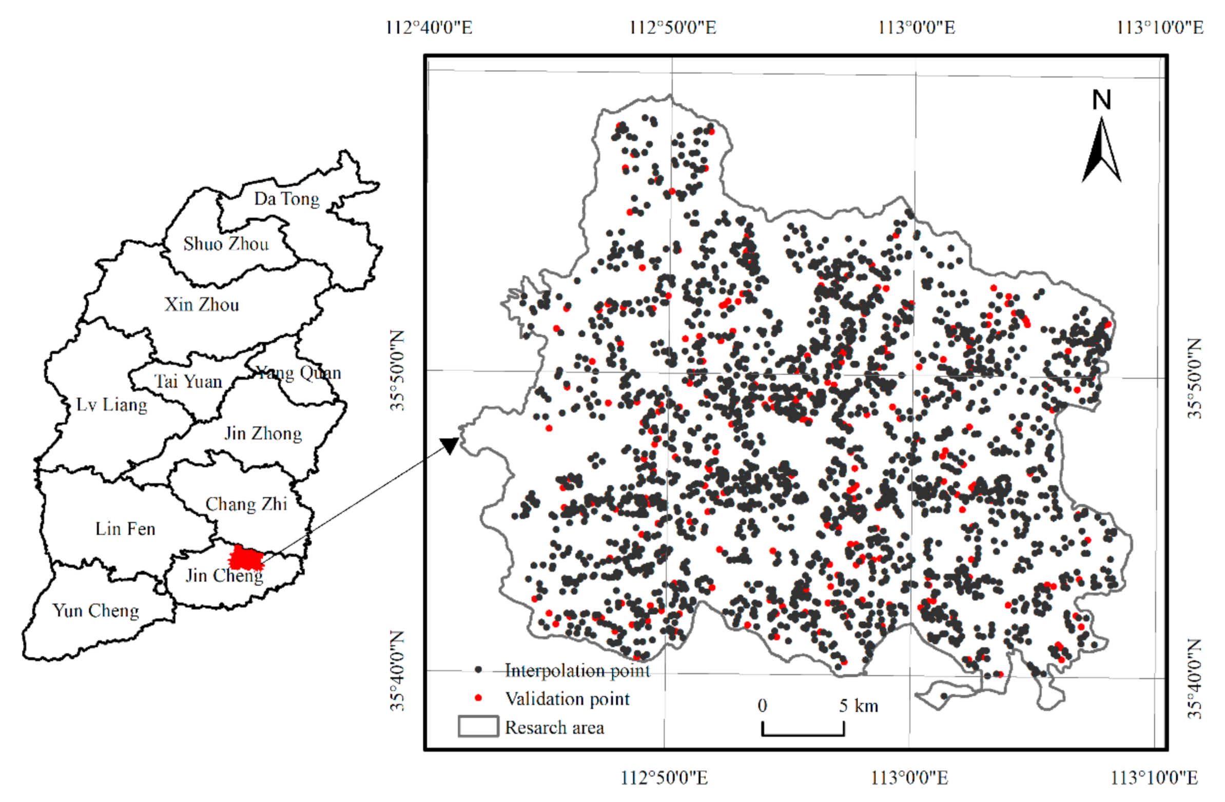
2.1. Study Area

Gaoping City is located at the foothills of the Taihang Mountains in the southeast area of Shanxi Province in central China (35°40′–36°0′ N, 112°40′–113°10′ E; Figure 1). The total land area of the city is 946 km², with an altitude ranging from 780 m to 1391 m. Gaoping is surrounded by mountains in the east, west, and north, with flat land in the middle. There are many types of land use and large areas of arable land. The main soil types are cinnamon soil and fluvo-aquic soil. The study area has a warm temperate continental monsoon climate. The annual average temperature is approximately 10.5 °C, the annual average sunshine duration is 2532.5 h, the frost-free period is 180–200 days, and the annual average rainfall is about 600 mm (mainly from July to September). Shanxi Province, Gaoping, where the research was carried out is characterized by good water and air quality and as such offers optimum research possibilities.

2.2. Data Sources

2.2.1. Soil Sampling and Determination

A total of 2583 samples were collected before crops were planted in the spring of 2010, in accordance with the “Rules for soil quality survey and assessment” (NY/T 1634–2008). We used the “S” method to layout points in each field by employing stainless steel soil drills and other tools. The spatial distribution of the data points is shown in Figure 1. After pretreatment of the soil samples, the contents of soil organic matter (SOM), total nitrogen (TN), available phosphorus (AP), and available potassium (AK) of each sample were determined. Specific determination methods are described elsewhere [40].

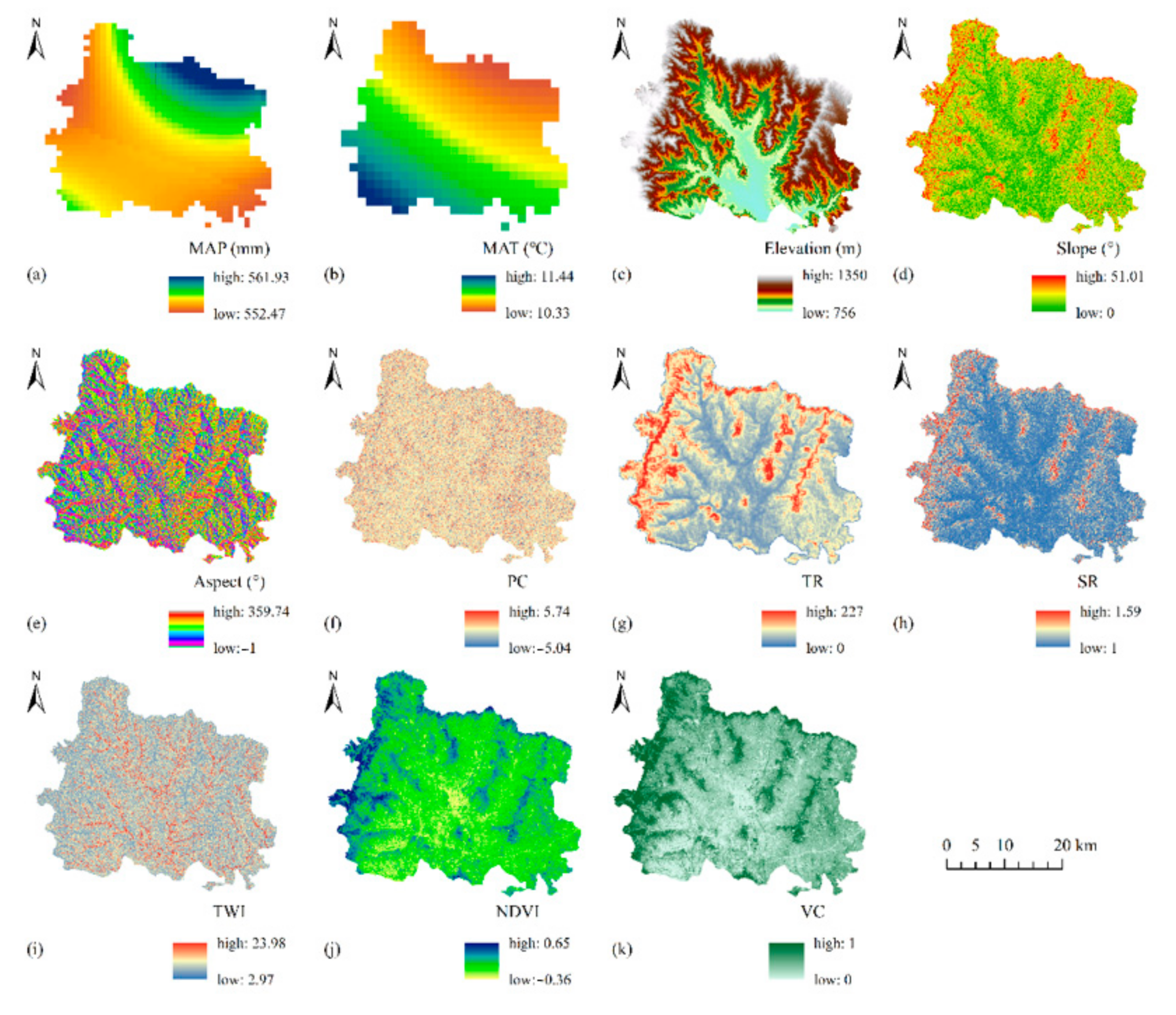
2.2.2. Environmental Data

Numerous studies have demonstrated that soil nutrient content is comprehensively affected by factors such as climate, vegetation, and terrain [3,14,41,42]. Therefore, this paper selected these factors as auxiliary variables to participate in the investigation of soil nutrient spatial modeling.

The climate factors included mean annual precipitation (MAP) and mean annual temperature (MAT), which were obtained from National Meteorological Information Center [43]. We downloaded the precipitation and temperature data of local meteorological stations from 1980 to 2010. By calculating the average multi-year precipitation and average multi-year temperature, and by performing kriging interpolation, meteorological data at each soil sampling point in Gaoping City were extracted.

The topographic factors were derived from the DEM (30 m spatial resolution) obtained from Geospatial Data Cloud [44]. Based on the DEM data, we obtained various composite terrain factor indicators in the SAGA-GIS software.

The remote-sensing data include the NDVI and vegetation coverage (VC), which were also derived from Geospatial Data Cloud [44]. We downloaded Landsat 8 remote sensing images that were consistent with the sampling time. After preprocessing the image, we used the band calculator to calculate the NDVI and VC to reflect the growth status of farmland vegetation in that year. The data of various environmental covariates are shown in

Table 1. List of environmental covariate data.

Data Type	Index
Terrain data	Elevation
	Slope
	Aspect
	Plane curvature, PC
	Topographic relief, TR
	Surface roughness, SR
	Topographic wetness index, TWI
Meteorological data	Mean average precipitation, MAP
	Mean average temperature, MAT
Remote sensing data	Normalized differential vegetation index, NDVI
	Vegetation coverage, VC

.

2.3. Geospatial Techniques

2.3.1. Ordinary Kriging (OK)

The OK model is based on spatial autocorrelation and second-order stationary assumptions. It uses the semivariogram theory as a tool to analyze its spatial structure, and realizes the optimal unbiased linear estimation of the unknown area based on the existing sampling point data in a limited area [11]. The semivariance function equation is described as Equation (1).

$$\gamma (h)=\frac{1}{2N(h)}{\displaystyle \sum _{i=1}^{N(h)}{\left[Z\left(x_i\right)-Z\left(x_i+h\right)\right]}^2}$$

(1)

where $\gamma \left(h\right)$ is the semivariogram value; $h$ is the lag; $N\left(h\right)$ is the total number of point pairs with an interval of $h$; $Z\left(x_i\right)$ and $Z\left(x_i+h\right)$ are the measured values of regionalized variables at positions $x_i$ and $x_i+h$, respectively.

2.3.2. Regression Kriging (RK)

Regression kriging combines multiple linear regression (MLR) and kriging interpolation. The steps for establishing this method are as follows: a stepwise MLR analysis is performed between the target variable and its highly correlated auxiliary variables to obtain the trend item and residual item, which represent certainty and randomness, respectively. Then, OK is applied to interpolate the residual item of the regression model before finally summing them up [16,18]. The fundamental equation of the RK model is described as Equation (2):

$$y_{RK}\left(x_i\right)=y_{MLR}\left(x_i\right)+y_{OK}\left(x_i\right)$$

(2)

where $y_{RK}\left(x_i\right)$ denotes the predicted value of the RK model at the point $x_i$; $y_{MLR}\left(x_i\right)$ is the trend value of MLR at point $x_i$; $y_{OK}\left(x_i\right)$ is the residual item estimated by the OK method at the point $x_i$.

2.3.3. Geographically Weighted Regression Kriging (GWRK)

As a hybrid method, the modeling process of GWRK [25] is similar to that of RK, with the exception of the fact that the global fitting in RK is replaced with the local fitting in GWR. The GWR approach is used to deal with spatial non-stationarity by introducing a spatial location into regression coefficients [21].

Assuming that there is a total of $n$ observation points, the location of each observation point is $\left(u_i,v_i\right)$, and there is a total of $m$ independent variables involved in modeling. The expression of the GWR model is shown in Equation (3):

$$y_i={\displaystyle \sum _{i=0}^n{\displaystyle \sum _{j=0}^m{\beta }_j}}\left(u_i,v_i\right)x_{ij}+{\epsilon }_i$$

(3)

where $x_{ij}$ is the jth independent variable at the observation point; ${\beta }_i\left(u_i,v_i\right)$ is the regression coefficient of the jth independent variable at the position $\left(u_i,v_i\right)$;${\epsilon }_i$ is the random error term; $y_i$ is dependent variable.

Two types of spatial weight function methods, the Gaussian function and Bi-square function, are usually used to determine the spatial weight in GWR analysis. Different types of kernel functions can be used during operation, including fixed kernel functions and adaptive kernel functions. Research has shown that an adaptive kernel is arguably more favorable when dealing with non-uniform spatial distributions [21,24]. Because the sampling points are not uniformly distributed, this study selects an adaptive Gaussian kernel function for modeling. In addition, geographic weighted regression analysis is very sensitive to the bandwidth selection of a specific weight function [45]. This study uses the corrected Akaike information criterion (AICc) to determine the model bandwidth, where the principle is to minimize the AICc. This approach helps to evaluate whether the GWR model simulates the data better than the MLR model.

2.3.4. Multiscale Geographically Weighted Regression Kriging (MGWRK)

As mentioned, MGWRK [39] is a combination of MGWR and kriging interpolation. The MGWR model can be expressed as Equation (4):

$$y_i={\displaystyle \sum _{i=0}^n{\displaystyle \sum _{j=0}^m{\beta }_{bwj}}}\left(u_i,v_i\right)x_{ij}+{\epsilon }_i$$

(4)

where ${\beta }_{bwj}$ is the regression coefficient corrected by the effective bandwidth of the jth independent variable. In our study, the kernel functions and kernel types of MGWR and GWR models are consistent.

The MGWR model accounts for the spatial scale effect of the influence of different independent variables on the dependent variable, and provides different independent variables with different bandwidths. This is the main difference between the MGWR model and the GWR model. All independent variables in the GWR model share a bandwidth, which can be regarded as a weighted average of different levels of spatial heterogeneity [38,46].

2.4. Model Validation and Evaluation

Ninety percent of sampling points (2284) were randomly selected from the original data as the prediction set to build the model, and the remaining 10% samples (254) were used as the verification set to test the model’s prediction accuracy. We evaluated the performance of different models by calculating the mean error (ME), mean absolute error (MAE), root mean square error (RMSE), and prediction accuracy (Acc) of the validation set [33,47]. These four indices can be written as Equations (5)–(8):

$$ME=\frac{1}{n}{\displaystyle \sum _{i=1}^n\left[\widehat{Z}\left(x_i\right)-Z\left(x_i\right)\right]}$$

(5)

$$MAE=\frac{1}{n}{\displaystyle \sum _{i=1}^n\left[\left|\widehat{Z}\left(x_i\right)-Z\left(x_i\right)\right|\right]}$$

(6)

$$RMSE=\sqrt{\frac{1}{n}{\displaystyle \sum _{i=1}^n{\left[\widehat{Z}\left(x_i\right)-Z\left(x_i\right)\right]}^2}}$$

(7)

$$Acc=\left[1-\frac{1}{n}{\displaystyle \sum _{i=1}^n\left|\frac{\widehat{Z}\left(x_i\right)-Z\left(x_i\right)}{Z\left(x_i\right)}\right|}\right]$$

(8)

where $\widehat{Z}$($x_i$) is the predicted value at position $x_i$; $Z\left(x_i\right)$ is the measured value at position $x_i$; $n$ is the number of samples.

In general, ME, MAE, and RMSE values closer to zero and a higher Acc give a better prediction.

3. Results

3.1. Descriptive Statistics

In this study, 11 indicators (elevation, slope, aspect, PC, TR, SR, TWI, MAP, MAT, NDVI, and VC) were initially selected as environmental variables (Figure 2).

Table 2. Descriptive statistics of soil nutrients.

Index	Unit	Min	Max	Mean	S.D.	Variance	CV (%)
Soil organic matter, SOM	g kg−1	3.10	45.00	27.04	7.28	52.99	26.92
Total nitrogen, TN	g kg−1	0.11	2.51	1.33	0.29	0.08	21.65
Avaliable Phosophorus, AP	mg kg−1	1.40	39.90	12.90	6.25	39.09	48.48
Avaliable potassium, AK	mg kg−1	38.00	388.00	153.03	44.30	1962.28	28.95

shows the descriptive statistics of the soil nutrients. The SOM content ranged from 3.10 g/kg to 45 g/kg. The TN, AP, and AK contents of soil ranged from 0.11 g/kg to 2.51 g/kg, 1.40 mg/kg to 39.90 mg/kg, and 38 mg/kg to 388 mg/kg, respectively. The coefficient of variation (CV) is defined as the ratio of the standard deviation to the mean, and is a normalized measure of the dispersion of a probability distribution or frequency distribution [20]. The CV values of the SOM, TN, AP, and AK contents were 26.92%, 21.65%, 48.48%, and 28.95%, respectively. Thus, the CV of the AP content was the largest, which is consistent with previous research results [48]. In addition,

Table 3. Descriptive statistics of soil environmental covariates.

Index	Unit	Min	Max	Mean	S.D.	Variance	CV (%)
Mean Average Precipitation, MAP	mm	552.52	561.93	555.35	1.67	2.79	0.30
Mean Average Temperature, MAT	°C	10.33	11.44	10.82	0.25	0.06	2.29
Elevation	m	780.00	1273.00	914.78	68.08	4635.17	7.44
Slope	°	0.00	34.20	7.38	4.46	19.87	60.41
Aspect	°	−1.00	359.17	176.34	96.16	9245.94	54.53
Surface Roughness, SR		1.00	1.21	1.01	0.02	0.00	1.49
Topographic relief, TR		14.00	157.00	46.24	18.69	349.19	40.41
Plane Curvature, PC		−2.24	2.34	0.01	0.57	0.33	5870.25
Topographic wetness index, TWI		3.81	22.38	7.44	2.68	7.16	35.95
Normalized differential vegetation index, NDVI		−0.16	0.37	0.07	0.07	0.01	100.89
Vegetation Coverage, VC		0.00	1.00	0.29	0.18	0.03	61.33

Notes: Min, Minimum. Max, Maximum. S.D., standard deviation. CV, the coefficient of variation.

shows the descriptive statistics of the environmental covariates. The CV of different environmental covariates in the study area also varied significantly.

3.2. Correlation Analysis of Soil Nutrients and Environmental Factors

The results of a Pearson’s correlation analysis of soil nutrients and environmental factors in the study area are presented in

Table 4. Correlations between environment attributes and soil nutrients.

Index	SOM	TN	AP	AK
MAP	0.114 **	−0.006	−0.098 **	−0.109 **
MAT	−0.015	0.018	0.082 **	0.079 **
Elevation	−0.154 **	−0.057 **	0.039	−0.025
Slope	−0.094 **	−0.022	−0.008	−0.012
Aspect	0.016	−0.002	0.012	0.015
SR	−0.082 **	−0.020	0.001	−0.016
TR	−0.214 **	−0.066 **	0.019	−0.029
PC	−0.028	−0.018	0.025	0.001
TWI	0.018	0.006	−0.031	−0.043 *
NDVI	−0.151 **	−0.098 **	−0.004	0.010
VC	−0.154 **	−0.098 **	−0.006	0.006

Notes of abbreviation. SOM, soil organic matter. TN, total nitrogen. AP, available phosophorus. AK, available potassium. MAP, mean average precipitation. MAT, mean average temperature. SR, surface roughness. TR, topographic relief. PC, plane curvature. TWI, topographic wetness index. NDVI, normalized differential vegetation index. VC, vegetation coverage. * and ** represent the significant at the 0.05 level and 0.01 level (2-tailed), respectively.

. There were significant correlations between the SOM content and (i) topographic factors (elevation, slope, SR, TR), (ii) climate factors (MAP), and (iii) vegetation factors (NDVI and VC). The significant influencing variables of the TN content of soil were elevation, TR, and the NDVI. Both MAP and MAT had significant effects on the AP and AK contents. The AP content was also significantly negatively correlated with the TWI.

Terrain conditions affect soil nutrients by regulating the distribution of soil moisture as well as heat and air permeability conditions in a landscape [49,50]. In this study, topographic factors and soil nutrient content were significantly negatively correlated, thus indicating that environments with a high elevation, steep slopes, a fragmented ground surface, or low TWI usually have a low soil nutrient content.

Climate is the main driving force affecting plant type, crop growth, and litter decomposition [51], but soil nutrients have different response mechanisms to the different synergy of temperature and precipitation. Generally speaking, an environment with high precipitation and low temperature is conducive to the accumulation of soil nutrients [49]; however, an increase in precipitation may also increase soil erosion, which leads to the loss of effective soil elements [52]. Studies have also shown that temperature changes will affect the decomposition of microorganisms in the soil, thus complicating the relationship between temperature and nutrients [53]. In our study, the MAP had a positive effect on the SOM content, whereas it had a negative effect on AP and AK. Temperature exhibited a significant positive relationship with AP and AK, while the relationships between SOM, TN, and temperature were not significant.

Vegetation is also an important factor affecting the soil nutrient content. The influence of vegetation is usually mediated through terrain and climate variables [54]. Significant negative correlations were observed between the various vegetation factors and the soil nutrient content in Gaoping City, which is inconsistent with the results of Bangroo et al. [14]. It may be that the part of the plant residues returned to the soil by complex vegetation types hindered the accumulation of soil nutrients.

3.3. Analysis of Spatial Distribution Patterns of Soil Nutrients

3.3.1. Selection of Environmental Covariates and MLR Modeling

Using a stepwise regression method to select variables can ensure that only independent variable factors that are significant to the soil nutrient content enter the regression model, and can also check the multicollinearity of the model [55]. The probability level of variable entry in stepwise regression is 0.05, and the probability level of elimination is 0.1 The final fitting model of the MLR of each dependent variable is shown in

Table 5. MLR models between soil nutrient and environmental variables.

Index	Regression Equation	R2
SOM	SOM = 0.7188 × MAP − 0.1338 × TWI − 0.0123 × Elevation − 0.1669 × Slope − 2.5425 × VC + 52.1433 × SR − 0.05106 × TR − 0.5255 × PC − 408.3766	0.075
TN	TN = 0.4060069 × NDVI + 1.354716	0.0097
AP	AP = −0.3824 × MAP + 1.5562 × MAT + 0.0123 × Elevation − 0.0170 × TR + 197.9734	0.0193
AK	AK = −2.9193 × MAP − 0.8736 × TWI − 0.0909 × TR + 1785.001	0.0154

Notes: SOM = soil organic matter, TN = total nitrogen, AP = available phosphorus, AK = available potassium; MAP = mean average precipitation, MAT = mean average temperature, SR = surface roughness, TR = topographic relief, PC = plane curvature, TWI = topographic wetness index, NDVI = normalized differential vegetation index, VC = vegetation coverage.

.

To further explore the influence of environmental covariates on the soil nutrient content in the study area at different locations, and to compare the differences in spatial mapping of different methods, the factors of the MLR model were also applied for GWR and MGWR modeling.

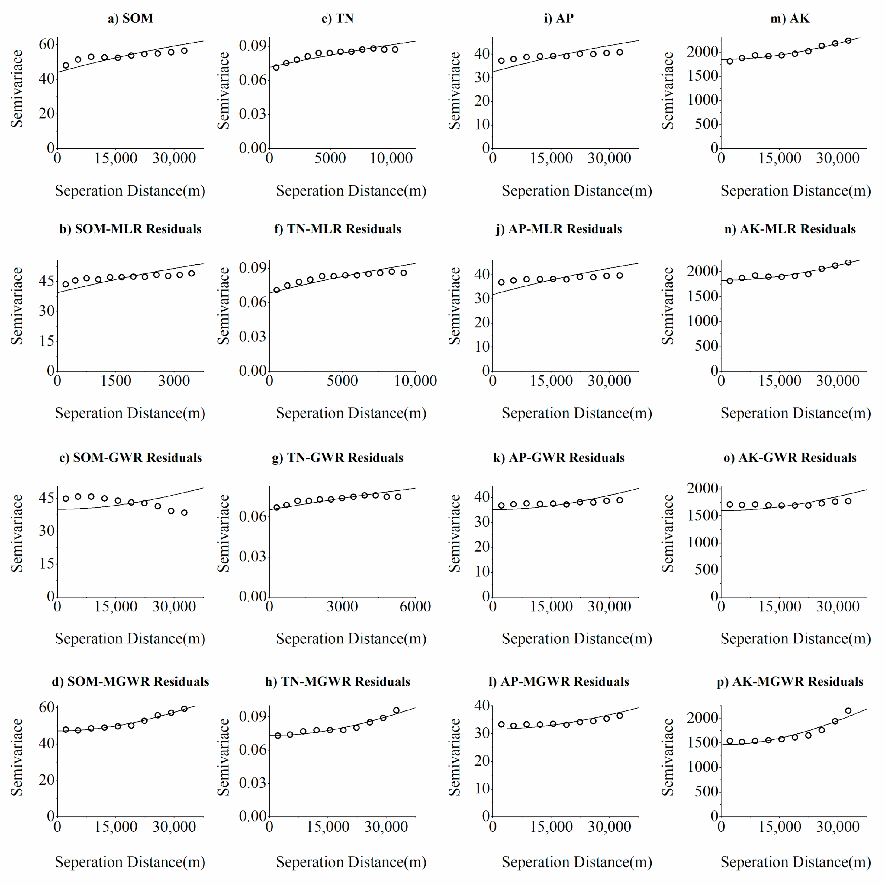
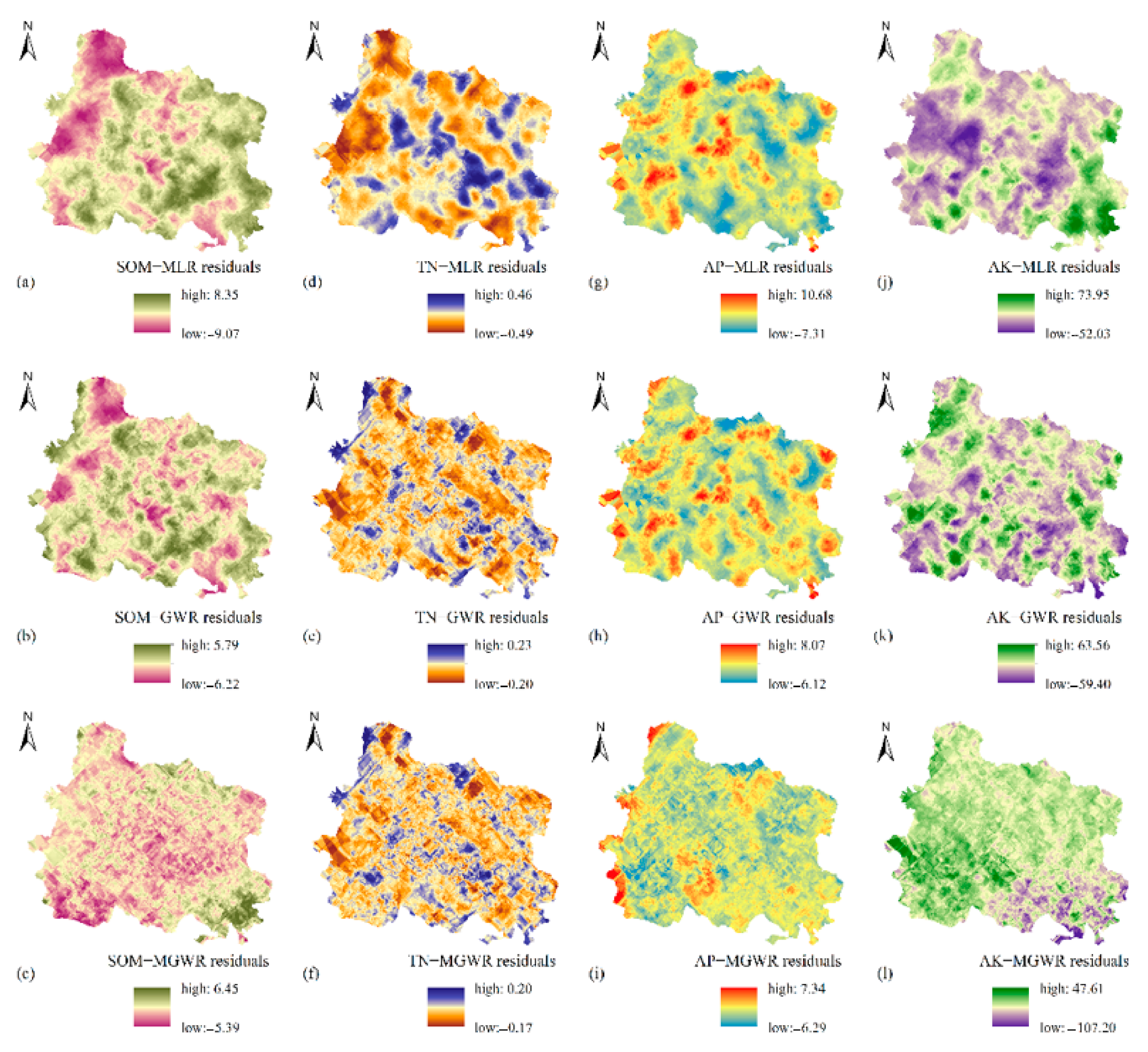
3.3.2. Spatial Variability Characteristics of Soil Nutrients and Residuals of MLR, GWR, and MGWR Models

The residuals of the regression models were used to fit the semivariogram model. We selected the optimal semivariogram model according to the maximum determination coefficient (R²).

Table 6. Semivariogram parameters of each model.

Index	Type	Fitting Model	Nugget (C0)	Sill (C0 + C)	Nugget/Sill [C0/(C0 + C), %]	Range (m)	R2
SOM	OK	Exponential Model	44.000	88.010	50.0	71,100	0.873
	MLR residuals	Exponential Model	39.300	78.610	50.0	8110	0.841
	GWR residuals	Gaussion Model	40.000	80.010	50.0	71,100	0.966
	MGWR residuals	Gaussion Model	47.200	109.980	57.1	71,100	0.979
TN	OK	Exponential Model	0.0715	0.143	50.0	31,100	0.844
	MLR residuals	Exponential Model	0.068	0.137	50.0	21,100	0.876
	GWR residuals	Exponential Model	0.065	0.131	50.0	21,100	0.837
	MGWR residuals	Gaussion Model	0.073	0.176	58.5	71,100	0.923
AP	OK	Exponential Model	32.500	65.010	50.0	71,100	0.941
	MLR residuals	Exponential Model	31.800	63.610	50.0	71,100	0.896
	GWR residuals	Gaussion Model	35.100	70.210	50.0	71,100	0.835
	MGWR residuals	Gaussion Model	31.630	63.270	50.0	71,100	0.883
AK	OK	Gaussion Model	1851	3882	52.3	71,100	0.959
	MLR residuals	Gaussion Model	1826	3653	50.0	71,100	0.915
	GWR residuals	Gaussion Model	1599	3199	50.0	71,100	0.850
	MGWR residuals	Gaussion Model	1462	4453	67.2	71,100	0.896

showed that the R² value of each model was >80%, which indicated that a good model simulation effect was achieved in each case. Semivariograms of soil nutrients and the residuals of MLR, GWR, and MGWR are shown in Figure 3.

The spatial autocorrelation for SOM in the various models ranged from 8110 m to 71,100 m. The nugget values were 44 (OK), 39.3 (MLR residuals), 40 (GWR residuals), and 47.2 (MGWR residuals). The spatial autocorrelation for TN ranged up to 31,100 m, and the spatial ranges of the residuals for MLR, GWR, and MGWR were 21,100 m, 21,100 m, and 71,100 m, respectively. The nugget values were 0.0715 (OK), 0.068 (MLR residuals), 0.065 (GWR residuals), and 0.073 (MGWR residuals). The spatial autocorrelation for the AP in each model ranged up to 71,100 m. The nugget values were 32.5 (OK), 31.8 (MLR residuals), 35.1 (GWR residuals), and 31.63 (MGWR residuals). The spatial autocorrelation for AK in each model also ranged up to 71,100 m. The nugget values were 1851 (OK), 1826 (MLR residuals), 1599 (GWR residuals), and 1462 (MGWR residuals).

The nugget/sill ratio of the optimal residual model was between 25% and 75%, which indicates that the model residual had a moderate degree of spatial autocorrelation. Therefore, it was necessary to use hybrid technologies (RK, GWRK, and MGWRK) for modeling [33]. The obtained semivariogram and various parameters were used to perform the kriging interpolation on the residuals. The results are presented in Figure 4, which shows that the three models produced very different spatial distributions of the residuals: (i) The extremum of the MLR residuals were the largest compared with other models, and the high and low values were clearly clustered, (ii) the spatial distribution of the GWR residuals presented a “low–high–staggered” phenomenon. (iii) the extremum of the MGWR residuals were the lowest for some indices, but the phenomenon of “low–high–staggered” distribution was much more serious than that of the GWR residuals. This may be because different bandwidths for various independent variables were used in the MGWR model, while all independent variables in the GWR model shared one mean bandwidth. Hence, the “fragmentation” phenomenon of the spatial distribution of GWR residuals was much less intense than that of the MGWR residuals.

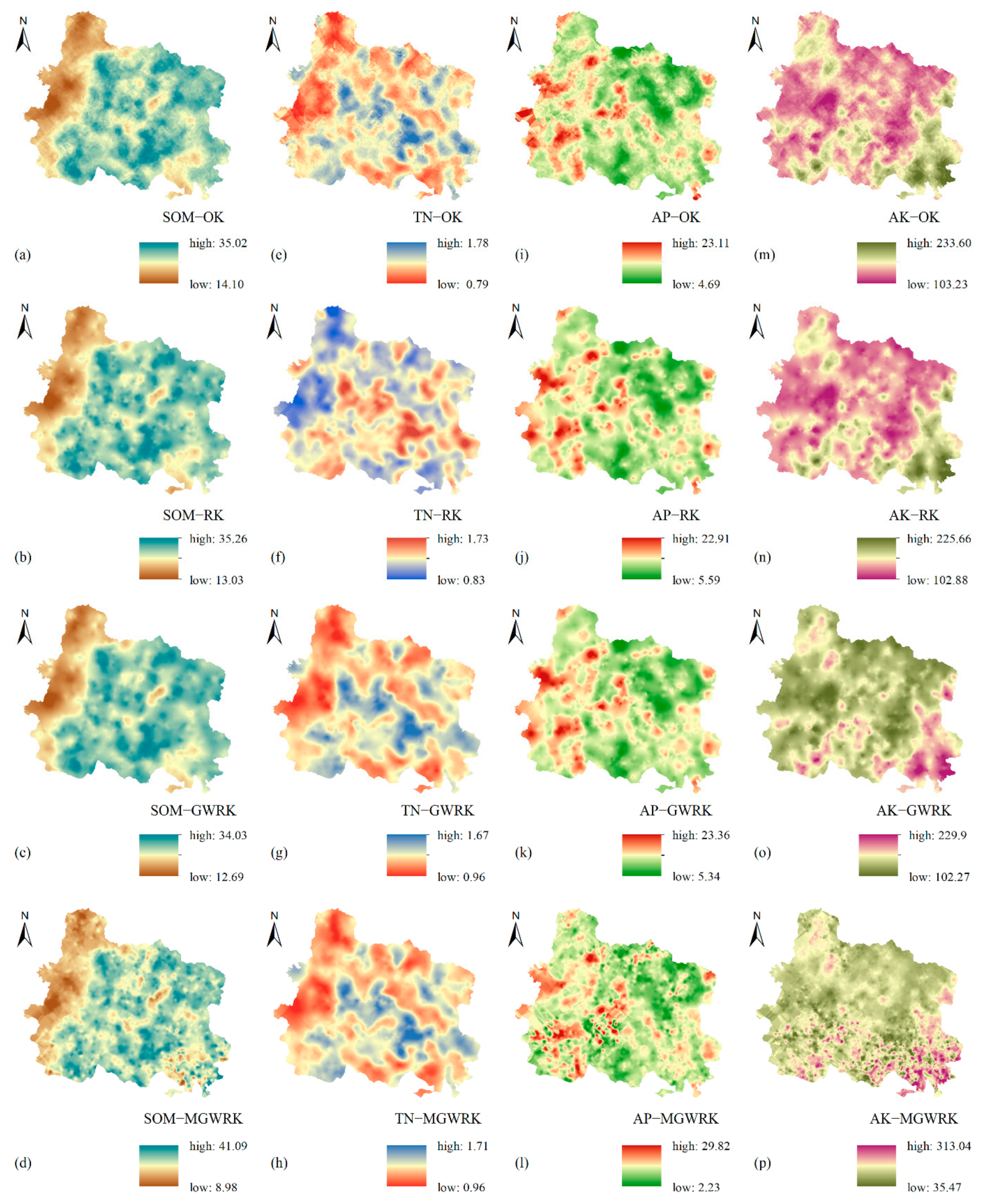
3.3.3. Results of Soil Nutrient Mapping Based on Different Models

Based on the above analysis, we drew spatial distribution maps of the soil nutrient content in the study area based on different geospatial technologies (OK, RK, GWRK, MGWRK) (Figure 5). A comparison of the results revealed that the overall spatial distribution trends of nutrient indicators obtained by these different models were consistent. The spatial prediction effect of the OK method was smoother. The mapping effects of RK and GWRK were very similar, while the “fragmentation” phenomenon of the MGWRK mapping effect was more prominent, which was basically consistent with the performance characteristics of the residual spatial distribution map.

The high-value areas of the SOM content in the study area were concentrated in the east, whereas the low-value areas were concentrated in the west. The TN content of soil decreased from the center of the study area toward the surrounding regions, which was contrary to the distribution patterns of various topographical factors. This implies that the TN content of soil in the study area is greatly affected by topographical factors. The AP content of soil in the western region of the study area was higher than that in the east, which was contrary to the characteristics of the spatial distribution of SOM. This may be because the regional differences in the amount of fertilizer applied, along with the fixed and difficult-to-move nature of phosphate fertilizers complicate the distribution of soil phosphorus over a small area [56,57]. The AK content was obviously higher in the southeast region of the study area compared to the northwest. The study also found that the soil nutrient content in the river valley is relatively high. This may be due to the flat terrain and convenient irrigation conditions, which is beneficial to the accumulation of various soil nutrient contents while soil nutrients are more likely to be lost in mountainous and hilly areas. At the same time, human activities such as different main crops and different management measures in various towns and small farm families may also cause differences in the spatial pattern of soil nutrient content.

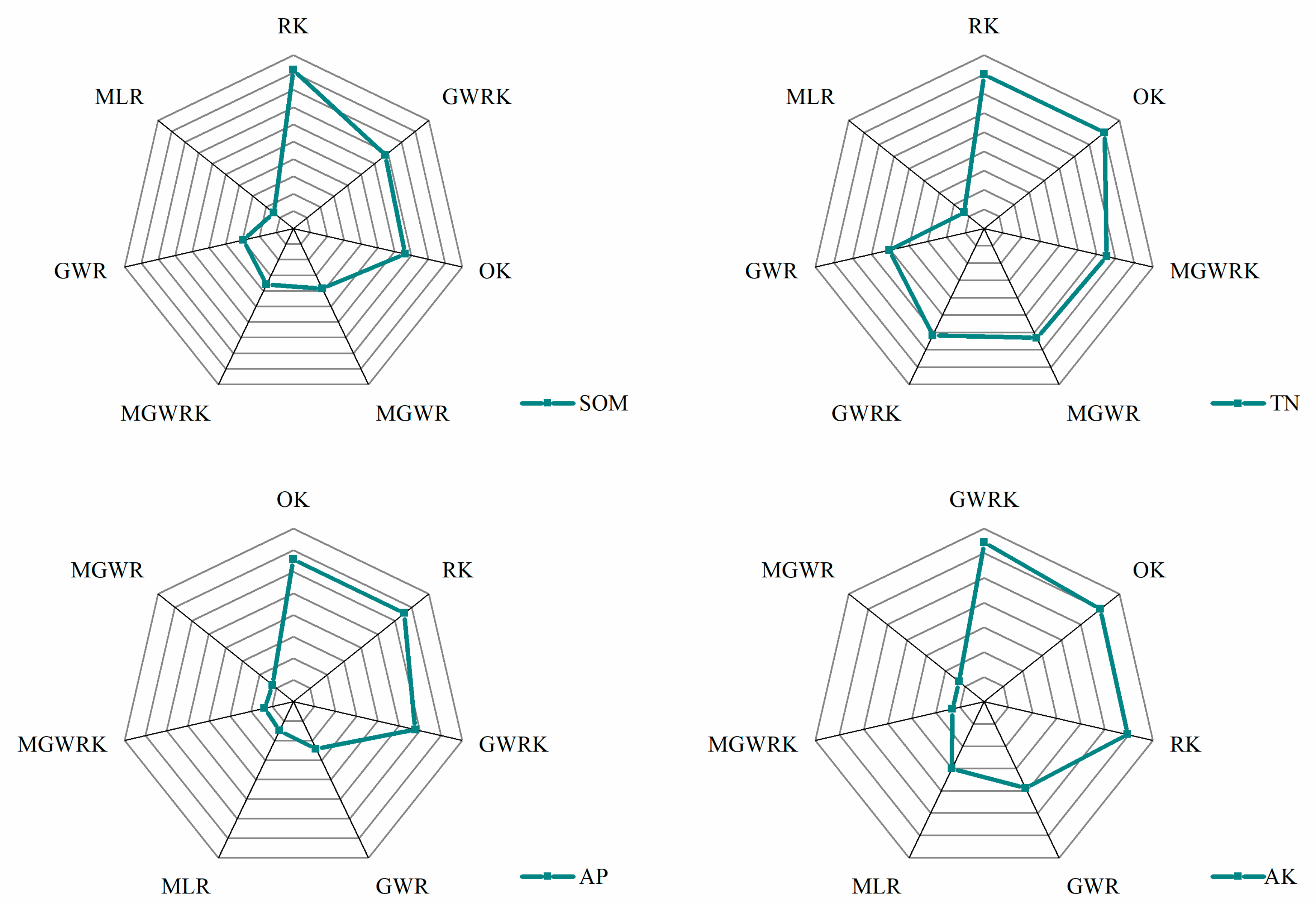
3.3.4. Evaluation of Model Accuracy

The prediction accuracy of the OK, RK, GWRK, and MGWRK models for soil nutrients was comprehensively evaluated by comparing each model’s performance based on the ME, MAE, RMSE, and Acc of 254 samples (

Table 7. Evaluation index of each model.

Index	Methods	ME	MAE	RMSE	ACC
SOM	OK	0.0232	4.4986	5.6669	0.8062
	MLR	−0.0001	5.6720	6.9999	0.7545
	RK	0.0160	3.9056	4.9402	0.8317
	GWR	0.0340	5.3505	6.6495	0.7696
	GWRK	0.0244	4.4597	5.6152	0.8079
	MGWR	0.1947	5.2317	6.6090	0.7785
	MGWRK	0.0186	5.2615	6.6687	0.7759
TN	OK	0.0003	0.1832	0.2392	0.8450
	MLR	−0.0003	0.2234	0.2858	0.8117
	RK	0.0004	0.1831	0.2388	0.8450
	GWR	−0.0019	0.1997	0.2598	0.8303
	GWRK	0.0010	0.1942	0.2530	0.8358
	MGWR	−0.0007	0.1928	0.2512	0.8365
	MGWRK	0.0007	0.1922	0.2504	0.8377
AP	OK	−0.0048	3.6354	4.8464	0.6716
	MLR	0.0000	4.6657	6.1906	0.5696
	RK	−0.0069	3.6383	4.8454	0.6712
	GWR	−0.0577	4.4876	5.9648	0.5883
	GWRK	−0.0086	3.8141	5.0737	0.6557
	MGWR	−0.0262	4.8092	6.3629	0.5645
	MGWRK	−0.0137	4.8087	6.3818	0.5674
AK	OK	0.0385	25.5836	33.9677	0.8200
	MLR	−0.0002	33.6282	43.9463	0.7601
	RK	0.0419	25.7632	34.1836	0.8188
	GWR	0.2043	31.4605	41.5619	0.7775
	GWRK	0.0508	24.3765	32.4621	0.8286
	MGWR	−1.5545	39.4682	53.3011	0.7260
	MGWRK	−0.1635	39.4764	53.5148	0.7264

Notes: OK: Ordinary Kriging; MLR: Multiple Linear Regression; RK: Regression Kriging; GWR: Geographically Weighted Regression; GWRK: Geographically Weighted Regression Kriging; MGWR: Multiscale Geographically Weighted Regression; MGWRK: Multiscale Geographically Weighted Regression Kriging.

). MLR, GWR, and MGWR participated in model accuracy evaluation simultaneously. The results showed that, for different soil properties, the best interpolation methods also differed depending on the selected auxiliary factors. We concluded that the best prediction model for (i) SOM was RK, (ii) TN and AP was RK or OK, and (iii) AK was GWRK.

4. Discussion

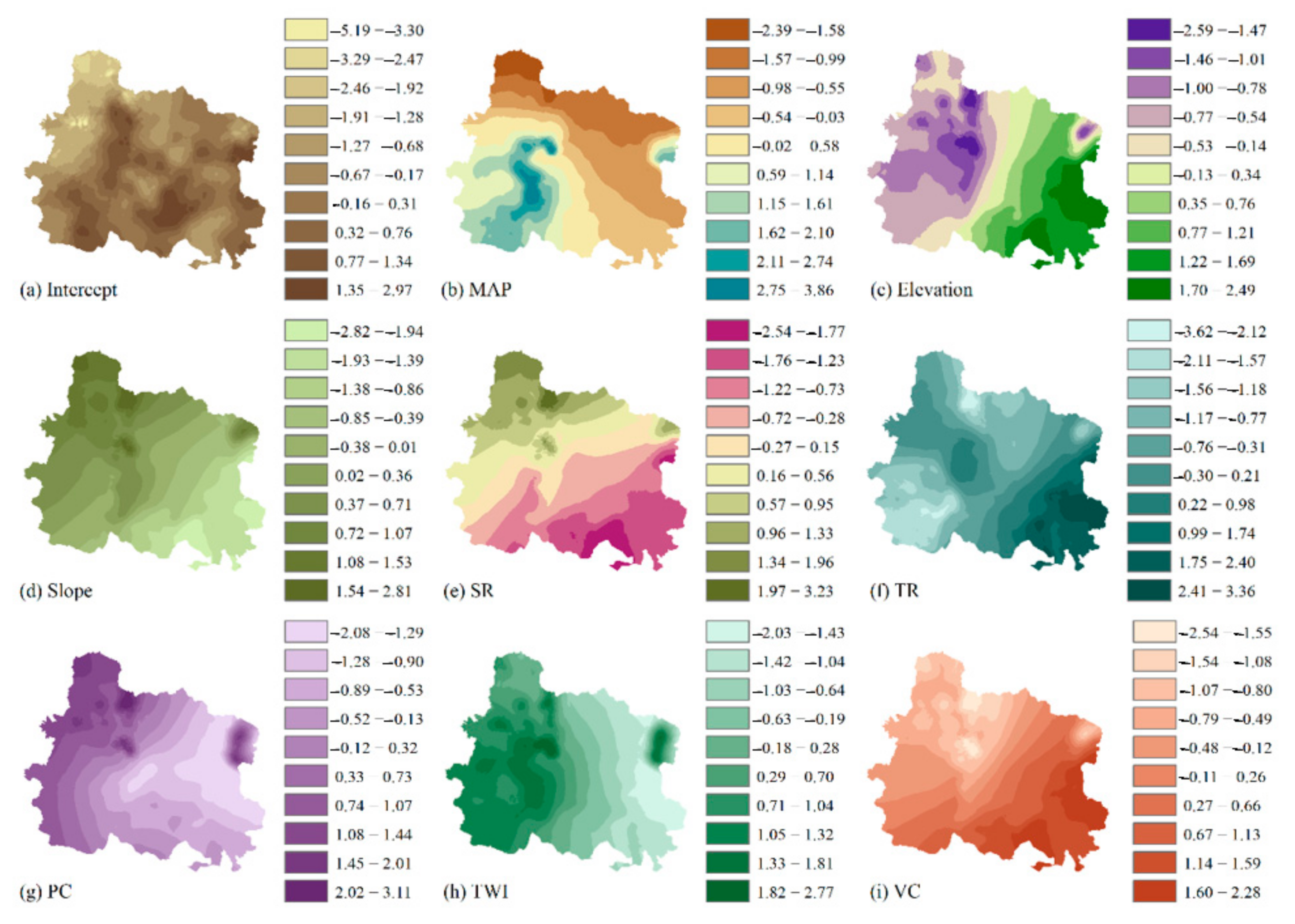
4.1. Spatial Non-Stationary Relationship between Soil Nutrients and Environmental Variables

In actual situations, the relationships between environmental variables and soil nutrients may vary geographically, i.e., spatial non-stationarity. Liu et al. [20] demonstrated in their study that nearest distance to residential area (TRA), Normalized Difference Moisture Index (NDMI), slope, Normalized Difference Vegetation Index (NDVI), nearest distance to road (TRD), and elevation were the dominant variables affecting the spatial distribution of SOC stocks; while the other three factors (i.e., nearest distance to river (TRR), aspect, and the land cover degree comprehensive index (LDCI)) did not play a dominant role in any part of the study region.

SOM is a critical indicator for the evaluation of soil quality. Thus, this study took SOM as an example to compare and analyze the regression effects of MLR, GWR and MGWR.

Table 8. The diagnostic criteria of the different regression models.

Model	RSS	AIC	AICC	R2	Adjust R2
MLR	2347.743	7022.766	7024.853	0.075	0.072
GWR	2118.583	6939.399	6947.297	0.165	0.132
MGWR	2028.812	6816.744	6823.630	0.201	0.171

Notes: RSS denotes residual sum of squares, AIC denotes Akaike information criterion, AICc is the corrected AIC.

showed that the GWR and MGWR models based on local regression idea could better explore and explain the spatial non-stationarity characteristics of variables than the global model MLR. It could also be seen from Table 7 that the MGWR model performed better than the GWR model in various diagnostic indicators. For example, the AICc value is reduced from 6947.297 (GWR) to 6823.630 (MGWR), and the R² value is increased from 0.165 (GWR) to 0.201 (MGWR), indicating that the MGWR model achieved a higher fitting accuracy. The maps of standardized local coefficients for the different explanatory variables by the MGWR model were provided in Figure 5, which could be a reference for the contribution of each influencing factor to SOM in various locations. The positive regression coefficients represent positive correlation, the negative regression coefficients correspond to negative correlation, and the absolute coefficient values reflect the degree of the influence of the factor on SOM [58].

Specifically, Figure 6b showed the standardized local coefficients of MAP (−2.39 to 3.86). MAP was negatively correlated with SOM in the northern region of the study area, and with the increasing MAP, the negative effect between MAP and SOM also increased. Whereas positive correlation was presented in the south, which indicated that SOM content increased with rising MAP over this area. Figure 6c showed the negative correlation between elevation and SOM in the western region, and the positive correlation in the eastern region. The local coefficients of slope (Figure 6d) and SR (Figure 6e) showed similar trends across the space. Both of them varied from positive to strongly negative from northwest to southeast, which demonstrated that with the increase of slope and MAP in the northwest of the study area, higher SOM could be observed, while the southeast is the opposite. In terms of TR (Figure 6f), negative correlation between SOM and TR was found in the north and southwest, while positive correlation was seen in the southeast. The absolute coefficient value was the lowest in the central area, which indicated that the central area was less effected by TR. Such spatial patterns could be due to the distribution of TR (Figure 2g); the terrain of the central region is very flat, therefore the weak influence from TR. In Figure 6g,h, it could be seen that the two explanatory variables (PC and TWI) had a strong negative impact on SOM in the eastern part of the study area and positive impact in the west. The negative effect in the eastern fringe was the greatest, which indicated that PC and TWI play a critical role in the distribution of SOM here. The local estimates of VC coefficients (Figure 6i) varied from strongly negative to strongly positive from northwest to southeast. We also found that the impact of VC on SOM is very weak in the central area, where the main land use type was construction land with low vegetation coverage. Understanding the characteristics of spatial non-stationarity is helpful to further explore the spatial relationships between environmental variables and soil nutrients.

4.2. Comparison of Model Performance in Soil Nutrient Mapping

Accuracy indicators were used to prepare radar charts to visualize the spatial prediction accuracy of the different models (Figure 7). The prediction accuracy of the MLR was not very good, and this approach provided the worst predictions of SOM and TN. Because MLR is less flexible, it can only estimate soil nutrient content by fitting a global function. If the relationship between soil properties and covariates is spatially variable rather than globally fixed, MLR usually cannot simulate the distribution of soil nutrients accurately. Although the regression equations and regression coefficients of the four nutrient indicators passed the significance test, the low R² values proved that each regression equation could only explain a small part of the spatial variation of the corresponding data [59]. This may be due to the non-linear relationship between soil nutrient indicators and environmental parameters in Gaoping City; thus, traditional linear regression models are restricted for the study area. However, by performing OK interpolation on the regression residuals, the prediction accuracy of the RK model was significantly improved, and similar conclusions have been drawn in previous studies [60,61,62,63].

The local regression model GWRK achieved a good prediction accuracy in most cases because it considered the non-stationarity of the spatial parameters, the relationship between each target variable and the explanatory variable, and the spatial distribution characteristics and trends of the residuals [12]. Brian et al. [23] used the GWRK method to predict the spatial pattern of soil pH at a depth of 15 cm. The results showed that, compared with the global model based on MLR, the local model based on GWR significantly improved the prediction accuracy of soil pH. Kumar et al. [24] estimated the SOC density in the Midwest of the United States based on the GWRK method. The authors proved that GWRK provides a useful visualization tool for SOC estimation on a regional scale when good correlations exist between SOC and environmental variables, and when the residual has spatial autocorrelation. These studies demonstrated that GWRK is a promising method for spatial predictions of soil attributes.

As a newly proposed method, MGWRK has certain advantages in reducing the overall residual level. The R² of MGWR is also higher than that of GWR, but its prediction accuracy is not very high compared with other models. Only in the prediction of TN, MGWRK ranked in the top three. The MGWRK model accounts for the spatial scale effect of different environmental covariates, which is a useful exploration. However, different bandwidths also have an impact on the spatial distribution of the residuals, which may lead to the failure of the MGWRK method to achieve the desired ideal effect. This was also reported by Qiao Lei et al. [39], who selected 13 indices (i.e., aspect, slope, MAP, MAT, altitude, annual cross primary productivity of vegetation, annual evapotranspiration, topographic wetness index, plane curvature, stream power index, terrain position index, terrain ruggedness index, and the annual average NDVI) as the environmental covariates, and compared the capabilities of OK, RK, GWRK, and MGWRK on SOM prediction; their results showed that the spatial prediction accuracy of the MGWRK method reached 69.0% of the RK method, 71.7% of the OK method, and 71.2% of the GWRK method. Therefore, MGWRK can provide a method reference for the digital mapping of the soil nutrient content in the study region, but its characteristics and performance require further investigation.

In summary, the use of hybrid technologies (RK, GWRK, and MGWRK) could improve the spatial prediction accuracy of soil properties than pure regression models (MLR, GWR, and MGWR). Hybrid methods also had advantages compared with OK, thus indicating that taking heterogeneity and dependence into consideration is necessary when model residuals showed moderate or strong spatial autocorrelation. Other studies reported similar results [23,64,65]. Yang et al. [33] compared the performance of MLR, RK, GWR, GWRK, MGWR, and MGWRK in mapping topsoil electrical conductivity (EC). The authors also found that hybrid approaches (i.e., MGWRK, RK, and GWRK) occupied the first three positions in the digital mapping of soil EC. However, the improvement of hybrid methods is very limited in our study, which may be due to the fuzzy correlations between soil properties and auxiliary variables [66]. The OK method, which makes full use of the spatial structure information of the data, has also achieved a satisfactory accuracy at a high sampling density and with a strong spatial correlation of the sampled data. Therefore, it may be more beneficial to design soil sampling rationally and obtain higher-quality data of auxiliary variables than to look for complex statistical methods to improve spatial prediction accuracy [10,67].

5. Conclusions

To summarize, this study compared the performance of OK, MLR, RK, GWR, GWRK, MGWR, and MGWRK for the digital mapping of soil nutrients in Gaoping City, China. The results showed that these models performed differently when predicting various indicators. The hybrid methods (RK, GWRK, and MGWRK) improved model prediction accuracy to a certain extent when the residuals were spatially correlated; however, this improvement was not significant. The new method MGWRK has certain advantages in reducing the overall residual level, but it failed to achieve the desired accuracy. Further verification of the applicable conditions and deviations of the MGWRK approach is required. Considering the cost of modeling, the OK method still provided an interpolation method with a relatively simple analysis process and relatively reliable results. This does not mean that more complex models would lead to an improved model performance.

In addition, the prediction accuracy of a spatial regression model largely depends on the correct selection of auxiliary variables. Although all the variables selected in this study were natural factors, soil nutrients are simultaneously affected by five major soil-forming factors and human factors. Human activities in low-altitude areas increase the spatial variability of soil nutrients. Future research should select appropriate methods to quantify management measures (e.g., planting systems, farming measurements), and then incorporate them into models to further improve prediction accuracy.

References

1. Mcbratney, A.B.; Odeh, I.O.A.; Bishop, T.F.A.; Dunbar, M.S.; Shatar, T.M. An overview of pedometric techniques for use in soil survey. Geoderma 2000, 97, 293–327. [Google Scholar] [CrossRef]
2. Sumfleth, K.; Duttmann, R. Prediction of soil property distribution in paddy soil landscapes using terrain data and satellite information as indicators. Ecol. Indic. 2008, 8, 485–501. [Google Scholar] [CrossRef]
3. John, K.; Isong, I.A.; Kebonye, N.M.; Ayito, E.O.; Agyeman, P.C.; Afu, S.M. Using Machine Learning Algorithms to Estimate Soil Organic Carbon Variability with Environmental Variables and Soil Nutrient Indicators in an Alluvial Soil. Land 2020, 9, 487. [Google Scholar] [CrossRef]
4. Liu, D.; Wang, Z.; Zhang, B.; Song, K.; Duan, H. Spatial distribution of soil organic carbon and analysis of related factors in croplands of the black soil region, Northeast China. Agric. Ecosyst. Environ. 2006, 113, 73–81. [Google Scholar] [CrossRef]
5. Liu, E.; Yan, C.; Mei, X.; He, W.; Bing, S.H.; Ding, L.; Qin, L.; Shuang, L.; Fan, T. Long-term effect of chemical fertilizer, straw, and manure on soil chemical and biological properties in northwest China. Geoderma 2010, 158, 173–180. [Google Scholar] [CrossRef]
6. Cambardella, C.; Moorman, T.B.; Novak, J.M.; Parkin, T.B.; Konopka, A. Field-Scale Variability of Soil Properties in Central Iowa Soils. Soilence Soc. Am. J. 1994, 58, 1501–1511. [Google Scholar] [CrossRef]
7. Wang, K.; Zhang, C.; Li, W. Comparison of Geographically Weighted Regression and Regression Kriging for Estimating the Spatial Distribution of Soil Organic Matter. Mapp. Sci. Remote Sens. 2012, 49, 915–932. [Google Scholar] [CrossRef]
8. Emadi, M.; Baghernejad, M. Comparison of spatial interpolation techniques for mapping soil pH and salinity in agricultural coastal areas, northern Iran. Arch. Agron. Soil Sci. 2014, 60, 1315–1327. [Google Scholar] [CrossRef]
9. Ye, H.; Huang, W.; Huang, S.; Huang, Y.; Zhang, S.; Dong, Y.; Chen, P. Effects of different sampling densities on geographically weighted regression kriging for predicting soil organic carbon. Spat. Stat. 2017, 20, 76–91. [Google Scholar] [CrossRef]
10. Shen, Q.; Wang, Y.; Wang, X.; Liu, X.; Zhang, X.; Zhang, S. Comparing interpolation methods to predict soil total phosphorus in the Mollisol area of Northeast China. Catena 2019, 174, 59–72. [Google Scholar] [CrossRef]
11. Eldeiry, A.A.; Garcia, L.A. Comparison of Ordinary Kriging, Regression Kriging, and Cokriging Techniques to Estimate Soil Salinity Using LANDSAT Images. J. Irrig. Drain. Eng. 2010, 136, 355–364. [Google Scholar] [CrossRef]
12. Kumar, A.; Lal, R.; Liu, D. A geographically weighted regression kriging approach for mapping soil organic carbon stock. Geoderma 2012, 189–190, 627–634. [Google Scholar] [CrossRef]
13. Watt, M.S.; Palmer, D.J. Use of regression kriging to develop a Carbon: Nitrogen ratio surface for New Zealand. Geoderma 2012, 183–184, 49–57. [Google Scholar] [CrossRef]
14. Bangroo, S.; Najar, G.; Achin, E.; Truong, P.N. Application of predictor variables in spatial quantification of soil organic carbon and total nitrogen using regression kriging in the North Kashmir forest Himalayas. Catena 2020, 193, 104632. [Google Scholar] [CrossRef]
15. Mondal, A.; Khare, D.; Kundu, S.; Mondal, S.; Mukherjee, S.; Mukhopadhyay, A. Spatial soil organic carbon (SOC) prediction by regression kriging using remote sensing data. Egypt. J. Remote Sens. Space Sci. 2017, 20, 61–70. [Google Scholar] [CrossRef] [Green Version]
16. Odeh, I.O.; McBratney, A.B.; Chittleborough, D.J. Further results on prediction of soil properties from terrain attributes: Heterotopic cokriging and regression-kriging. Geoderma 1995, 67, 215–226. [Google Scholar] [CrossRef]
17. Hengl, T.; Heuvelink, G.B.; Stein, A. A generic framework for spatial prediction of soil variables based on regression-kriging. Geoderma 2004, 120, 75–93. [Google Scholar] [CrossRef] [Green Version]
18. Hengl, T.; Heuvelink, G.B.M.; Rossiter, D.G. About regression-kriging: From equations to case studies. Comput. Geosci. 2007, 33, 1301–1315. [Google Scholar] [CrossRef]
19. Walter, C.; Mcbratney, A.B.; Donuaoui, A.; Minasny, B. Spatial prediction of topsoil salinity in the Chelif Valley, Algeria, using local ordinary kriging with local variograms versus whole-area variogram. Soil Res. 2001, 39, 259–272. [Google Scholar] [CrossRef] [Green Version]
20. Liu, Y.; Guo, L.; Jiang, Q.; Zhang, H.; Chen, Y. Comparing geospatial techniques to predict SOC stocks. Soil Tillage Res. 2015, 148, 46–58. [Google Scholar] [CrossRef]
21. Brunsdon, C.; Fotheringham, A.S.; Charlton, M.E. Geographically Weighted Regression: A Method for Exploring Spatial Nonstationarity. Geogr. Anal. 1996, 28, 281–298. [Google Scholar] [CrossRef]
22. Kumar, S.; Lal, R. Mapping the organic carbon stocks of surface soils using local spatial interpolator. J. Environ. Monit. JEM 2011, 13, 3128–3135. [Google Scholar] [CrossRef]
23. Odhiambo, B.O.; Kenduiywo, B.K.; Were, K. Spatial prediction and mapping of soil pH across a tropical afro-montane landscape. Appl. Geogr. 2020, 114, 102129. [Google Scholar] [CrossRef]
24. Kumar, S. Estimating spatial distribution of soil organic carbon for the Midwestern United States using historical database. Chemosphere 2015, 127, 49–57. [Google Scholar] [CrossRef] [PubMed]
25. Mitran, T.; Mishra, U.; Lal, R.; Ravisankar, T.; Sreenivas, K. Spatial distribution of soil carbon stocks in a semi-arid region of India. Geoderma Reg. 2018, 15, e00192. [Google Scholar] [CrossRef]
26. Yu, H.; Fotheringham, A.S.; Li, Z.; Oshan, T.; Kang, W.; Wolf, L.J. Inference in multiscale geographically weighted regression. Geogr. Anal. 2020, 52, 87–106. [Google Scholar] [CrossRef]
27. Mcmaster, R.B.; Sheppard, E. Introduction: Scale and Geographic Inquiry; Blackwell Publishing Ltd.: Hoboken, NJ, USA, 2008. [Google Scholar]
28. Lam, N.S.N.; Quattrochi, D.A. On the Issues of Scale, Resolution, and Fractal Analysis in the Mapping Sciences. Prof. Geogr. 1992, 44, 88–98. [Google Scholar] [CrossRef]
29. Peng, G.; Ling, B. Scale Effects on Spatially Embedded Contact Networks. Comput. Environ. Urban Syst. 2016, 59, 142–151. [Google Scholar] [CrossRef] [Green Version]
30. Cao, C. Detecting the Scale and Resolution Effects in Remote Sensing and GIS; Louisiana State University and Agricultural & Mechanical College: Baton Rouge, LA, USA, 1992. [Google Scholar]
31. Pan, Y.; Roth, A.; Yu, Z.; Doluschitz, R. The impact of variation in scale on the behavior of a cellular automata used for land use change modeling. Comput. Environ. Urban Syst. 2010, 34, 400–408. [Google Scholar] [CrossRef]
32. Murakami, D.; Lu, B.; Harris, P.; Brunsdon, C.; Charlton, M.; Nakaya, T.; Griffith, D.A. The importance of scale in spatially varying coefficient modeling. Ann. Am. Assoc. Geogr. 2019, 109, 50–70. [Google Scholar] [CrossRef]
33. Yang, S.-H.; Liu, F.; Song, X.-D.; Lu, Y.-Y.; Li, D.-C.; Zhao, Y.-G.; Zhang, G.-L. Mapping topsoil electrical conductivity by a mixed geographically weighted regression kriging: A case study in the Heihe River Basin, northwest China. Ecol. Indic. 2019, 102, 252–264. [Google Scholar] [CrossRef]
34. Mei, C.L.; He, S.Y.; Fang, K.T. A Note on the Mixed Geographically Weighted Regression Model. J. Reg. Sci. 2004, 44, 143–157. [Google Scholar] [CrossRef]
35. McMillen, D.P. Geographically Weighted Regression: The Analysis of Spatially Varying Relationships. Am. J. Agric. Econ. 2004, 86, 554–556. [Google Scholar] [CrossRef]
36. Nakaya, T.; Fotheringham, S.; Charlton, M.; Brunsdon, C. Semiparametric Geographically Weighted Generalised Linear Modelling in GWR 4.0. 2009. Available online: http://www.geocomputation.org/2009/PDF/nakaya_et_al.pdf (accessed on 15 October 2020).
37. Wu, C.; Ren, F.; Hu, W.; Du, Q. Multiscale geographically and temporally weighted regression: Exploring the spatiotemporal determinants of housing prices. Int. J. Geogr. Inf. Sci. 2019, 33, 489–511. [Google Scholar] [CrossRef]
38. Fotheringham, A.S.; Yang, W.; Wei, K. Multiscale Geographically Weighted Regression (MGWR). Ann. Am. Assoc. Geogr. 2017, 107, 1247–1265. [Google Scholar] [CrossRef]
39. Qiao, L.; Zhang, W.; Huang, M.; Wang, G.; Ren, J. Mapping of soil organic matter and its driving factors study based on MGWRK. Sci. Agric. Sin. 2020, 53, 1830–1844. [Google Scholar] [CrossRef]
40. Carter, M.R.; Gregorich, E.G. Soil Sampling and Methods of Analysis; CRC Press: Boca Raton, FL, USA, 2007. [Google Scholar]
41. Yang, S.; Zhang, H.; Zhang, C.; Li, W.; Guo, L.; Chen, J. Predicting soil organic matter content in a plain-to-hill transition belt using geographically weighted regression with stratification. Arch. Agron. Soil Sci. 2019, 65, 1745–1757. [Google Scholar] [CrossRef]
42. Zeng, C.; Yang, L.; Zhu, A.X.; Rossiter, D.G.; Liu, J.; Liu, J.; Qin, C.; Wang, D. Mapping soil organic matter concentration at different scales using a mixed geographically weighted regression method. Geoderma 2016, 281, 69–82. [Google Scholar] [CrossRef]
43. National Meteorological Information Center. Available online: http://data.cma.cnr (accessed on 15 October 2020).
44. Geospatial Data Cloud. Available online: http://www.gscloud.cn (accessed on 15 October 2020).
45. Shabrina, Z.; Buyuklieva, B.; Ng, M.K.M. Short-Term Rental Platform in the Urban Tourism Context: A Geographically Weighted Regression (GWR) and a Multiscale GWR (MGWR) Approaches. Geogr. Anal. 2020, 1–22. [Google Scholar] [CrossRef]
46. Oshan, T.M.; Li, Z.; Kang, W.; Wolf, L.J.; Fotheringham, A.S. MGWR: A Python Implementation of Multiscale Geographically Weighted Regression for Investigating Process Spatial Heterogeneity and Scale. Int. J. Geo Inf. 2019, 8, 269. [Google Scholar] [CrossRef] [Green Version]
47. Sun, Y.S.; Wang, W.F.; Li, G.C. Spatial distribution of forest carbon storage in Maoershan region, Northeast China based on geographically weighted regression kriging model. Chin. J. Appl. Ecol. 2019, 30, 1642–1650. [Google Scholar] [CrossRef]
48. Wang, S.; Hu, K.; Lu, P.; Yu, T. Spatial variability of soil available phosphorus and environmental risk analysis of soil phosphorus in Pinggu County of Beijing. Sci. Agric. Sin. 2009, 42, 1290–1298. [Google Scholar] [CrossRef]
49. Wang, S.; Adhikari, K.; Wang, Q.; Jin, X.; Li, H. Role of environmental variables in the spatial distribution of soil carbon (C), nitrogen (N), and C:N ratio from the northeastern coastal agroecosystems in China. Ecol. Indic. Integr. Monit. Assess. Manag. 2018, 84, 263–272. [Google Scholar] [CrossRef]
50. Tu, C.; He, T.; Lu, X.; Luo, Y.; Smith, P. Extent to which pH and topographic factors control soil organic carbon level in dry farming cropland soils of the mountainous region of Southwest China. Catena 2018, 163, 204–209. [Google Scholar] [CrossRef]
51. Song, X.D.; Brus, D.J.; Liu, F.; Li, D.C.; Zhao, Y.G.; Yang, J.L.; Zhang, G.L. Mapping soil organic carbon content by geographically weighted regression: A case study in the Heihe River Basin, China. Geoderma 2016, 261, 11–12. [Google Scholar] [CrossRef]
52. Naipal, V.; Ciais, P.; Wang, Y.; Lauerwald, R.; Oost, K.V. Global soil organic carbon removal by water erosion underclimate change and land use change during 1850–2005 AD. Biogeosci. Discuss. 2018, 4459–4480. [Google Scholar] [CrossRef] [Green Version]
53. Davidson, E.A.; Janssens, I.A. Temperature sensitivity of soil carbon decomposition and feedbacks to climate change. Nature 2006, 440, 165–173. [Google Scholar] [CrossRef] [PubMed]
54. Schillaci, C.; Acutis, M.; Lombardo, L.; Lipani, A.; Fantappiè, M.; Märker, M.; Saia, S. Spatio-temporal topsoil organic carbon mapping of a semi-arid Mediterranean region: The role of land use, soil texture, topographic indices and the influence of remote sensing data to modelling. Sci. Total Environ. 2017, 601–602, 821–832. [Google Scholar] [CrossRef]
55. Agostinelli, C. Robust stepwise regression. J. Appl. Stat. 2003, 48, 557–558. [Google Scholar] [CrossRef] [Green Version]
56. Behera, S.K.; Singh, M.V.; Singh, K.N.; Todwal, S. Distribution variability of total and extractable zinc in cultivated acid soils of India and their relationship with some selected soil properties. Geoderma 2012, 162, 242–250. [Google Scholar] [CrossRef]
57. Zhao, Q.; Zhao, G.; Jiang, H. Study on spatial variability of soil nutrients and reasonable sampling number at county scale. J. Nat. Resour. 2012, 27, 1382–1391. [Google Scholar] [CrossRef]
58. Qu, M.; Li, W.; Zhang, C.; Huang, B.; Zhao, Y. Spatial assessment of soil nitrogen availability and varying effects of related main soil factors on soil available nitrogen. Environ. Sci. Process. Impacts 2016, 18, 1449–1457. [Google Scholar] [CrossRef] [PubMed]
59. Hengl, T. A Practical Guide to Geostatistical Mapping of Environmental Variables; European Commission, Joint Research Centre, Institute for Environment and Sustainability: Ispra, Italy, 2007. [Google Scholar]
60. Zhang, S.; Wang, Z.; Zhang, B.; Song, K.; Liu, D.; Li, F.; Ren, C.; Huang, J.; Zhang, H. Prediction of spatial distribution of soil nutrients using terrain attributes and remote sensing data. Trans. Chin. Soc. Agric. Eng. 2010, 26, 188–194. [Google Scholar] [CrossRef]
61. Ren, L.; Yang, L.; Wang, H.; Yang, F.; Chen, W.; Zhang, L.; Jinhao, X.U. Spatial prediction of soil organic matter in apple region based on random forest. Resour. Environ. Arid Region 2018. [Google Scholar] [CrossRef]
62. Yang, Q.; Wang, X.Q.; Sun, X.L.; Wang, H.L. Comparing Prediction Accuracies of Ordinary Kriging and Regression Kriging with REML in Soil Properties Mapping. Chin. J. Soil Sci. 2018, 49, 283–292. [Google Scholar] [CrossRef]
63. Ziadat, M.F. Analyzing Digital Terrain Attributes to Predict Soil Attributes for a Relatively Large Area. Soil Sci. Soc. Am. J. 2005, 69, 1590–1599. [Google Scholar] [CrossRef]
64. Benítez, F.L.; Anderson, L.O.; Formaggio, A.N.R. Evaluation of geostatistical techniques to estimate the spatial distribution of aboveground biomass in the Amazon rainforest using high-resolution remote sensing data. Acta Amaz. 2016, 46, 151–160. [Google Scholar] [CrossRef] [Green Version]
65. Imran, M.; Stein, A.; Zurita-Milla, R. Using geographically weighted regression kriging for crop yield mapping in West Africa. Int. J. Geogr. Inf. Syst. 2015, 29, 234–257. [Google Scholar] [CrossRef]
66. Kravchenko, A.N.; Robertson, G.P. Can Topographical and Yield Data Substantially Improve Total Soil Carbon Mapping by Regression Kriging? Agron. J. 2007, 99, 12–17. [Google Scholar] [CrossRef] [Green Version]
67. Zhang, C.-T.; Yang, Y. Can the spatial prediction of soil organic matter be improved by incorporating multiple regression confidence intervals as soft data into BME method? Catena 2019, 178, 322–334. [Google Scholar] [CrossRef]
Figure 1. Location of the study area and the spatial distribution of the calibration points (n = 2284) and validation points (n = 254) in the study area.
Sustainability 13 03270 g001
Figure 2. Spatial distribution of environmental covariates.
Sustainability 13 03270 g002
Figure 3. Semivariograms of soil nutrients and the residuals of MLR, GWR, and MGWR.
Sustainability 13 03270 g003
Figure 4. Maps of different model residuals for soil nutrients.
Sustainability 13 03270 g004
Figure 5. Distribution of soil nutrients mapped by different models.
Sustainability 13 03270 g005
Figure 6. Spatial patterns of local coefficients in the MGWR.
Sustainability 13 03270 g006
Figure 7. Radar chart of the prediction accuracy (Acc) values of different models, where a longer polyline corresponds to greater accuracy. Notes: OK: Ordinary Kriging; MLR: Multiple Linear Regression; RK: Regression Kriging; GWR: Geographically Weighted Regression; GWRK: Geographically Weighted Regression Kriging; MGWR: Multiscale Geographically Weighted Regression; MGWRK: Multiscale Geographically Weighted Regression Kriging.
Sustainability 13 03270 g007