Sustainable Urban Greening and Cooling Strategies for Thermal Comfort at Pedestrian Level

Abstract

The increase of the urban warming phenomenon all over the world is gaining increasing attention from scientists as well as planners and policymakers due to its adverse effects on energy consumption, health, wellbeing, and air pollution. The protection of urban areas from the outdoor warming phenomenon is one of the challenges that policy and governments have to tackle as soon as possible and in the best possible way. Among the urban heat island mitigation techniques, cool materials and urban greening are identified as the most effective solutions in reducing the urban warming phenomenon. The effects produced by the adoption of cool materials and urban forestation on the urban microclimate were investigated through a computational fluid-dynamic (CFD) model. The CFD model was calibrated and validated thanks to experimental surveys within the Catania University campus area. The urban microclimate thermal comfort analysis and assessment were carried out with the Klima–Michel Model (KMM) and Munich Energy Balance Model for Individuals (MEMI). In particular, three scenarios were performed: cool, low, and high levels of urban greening. The cool scenario, although it produces air temperature at around 1.00 °C, determines the worst condition of outdoor thermal comfort, especially at the pedestrian level. On the contrary, a high level of urban greening, obtained by the extensive green roofs together with an urban forestation, guarantees the wellbeing of pedestrians, showing more convenient values of PMV and PET.

1. Introduction

The increase of urban population all over the world is leading to environmental, energy, and health implications of urban warming [1]. A recent study has shown that heatwaves, which are estimated to become more frequent and last longer in a hot climate, interact with urban warming to produce rather high heat stress for urban residents [2].

Furthermore, the features of the urbanized environments exacerbate the effects of global climate change [3]. Urban areas tend to have air temperatures higher than the rural surroundings as a result of gradual ground changes that include replacing the vegetation with buildings and roads [4].

The increase in temperatures in urban spaces is known as urban heat island (UHI) [5]. This phenomenon is due to several factors such as the specific composition of urban areas in terms of people and activities, morphology of neighborhoods, geometries, urban canyons [6], as well as surfaces with low albedo [7]. On a clear summer afternoon, the air temperature in a typical city could come up 2.5 °C higher than in the surrounding rural areas [8]. These factors affect the urban climate, energy uses, and livability of cities [9]. Urban areas are often characterized by higher vehicular traffic and less vegetation than their surrounding environment [10].

The radiative properties of the surface used in outdoor spaces have a key role, as they influence the air temperature of the lowest layers of the urban canopy layer [11]. Road pavements, claddings of facades, and roofs of the buildings are fundamental in the energy balance of the urban areas. The materials absorb solar radiation and store and release it by means of infrared radiation and convection heat transfer to their surrounding area during the evening and night-time [12]. Urban surfaces are characterized by values of solar absorption higher than rural surfaces [13]. Thereby, they have a superficial temperature lower than that of the building surfaces. Building materials emit an amount of energy higher than rural surfaces, and it leads to persistent warming in urban areas [14].

Increased urban temperatures produce the rising of the energy demand for building cooling, which in turn increases the greenhouse gas emissions and the outdoor thermal discomfort [15,16].

For evaluating outdoor thermal comfort in the urban contexts, several models are available in the scientific literature. Fanger’s indexes based on a steady-state energy balance model are implemented in many international standards [17,18]. Currently, the original equation of Fanger indexes is modified by Jendritzky and Nubler, 1981 [19,20], to evaluate the thermal comfort in external environments. They have produced the Klima–Michel Model (KMM) by adding the complex radiation balance in the outdoor environment and considering basic thermoregulatory processes through the human body, such as the constriction or dilation of peripheral blood vessels and the rate of physiological sweat [21].

The “Munich Energy-Balance Model for Individuals” (MEMI) [22,23] is the basis for the calculation of another index, called Physiological Equivalent Temperature (PET), which collected all the meteo-climatic factors in a single temperature index, namely the equivalent temperature. In KMM and MEMI models, the thermoregulatory processes are evaluated considering the human activity and climatic conditions.

Nowadays, mitigation strategies such as cool and green surfaces can enhance the outdoor thermal comfort in the urban areas, since both strategies reduce the sensible heat reaching the building surfaces, but the processes for reducing UHI are different [24]. Cool materials increase the reflectiveness of incoming solar radiation in urban areas reducing the net radiation [25]. Green surfaces increase the latent heat flux through the evapotranspiration process, while, thanks to the shading effect, reducing the incoming net radiation [26]. Cool materials applied on road pavements, with reflectivity 0.60, prove to be able to reduce the surface temperature by 5–6 °C compared to the conventional asphalt road [11]. In the Greek city of Florina, the application of cool pavements and cool roofs led to a reduction in the maximum air temperature by 1.39 °C and a decrease in soil temperature by 3.52 °C [27]. In Acharnes (Greece), reflective materials on the roofs allowed a reduction in surface temperature on the roofs between 1.51 °C to 10 °C and a decrease of 17% in energy consumptions [28]. The analysis of several mitigation strategies such as green roofs, green park, cool roofs, and cool pavements in an old densely populated neighborhood of Avola (Italy) highlighted that cool pavements reduce the environmental air temperature by over 2.0 °C [29]. Nevertheless, cool pavements can induce thermal discomfort to pedestrians and residents because of the high reflected solar radiation [30].

The adoption of vegetation in urban areas produces significant benefits by lowering air temperature and reducing air conditioning in the building [26,31]. It was found that medium trees and shrubs can cool down cities by from about 0.3 °C to 1.0 °C [4]. The results of CFD simulations on the effectiveness of several different mitigation strategies on the microclimate in Vienna showed that, at the pedestrian level, the planting trees allow achieving a decrease in air temperature of about 0.7 °C. A slight cooling in the air temperature, about 0.3 °C, was found when applying green roofs on all buildings of the investigated area. Moreover, the combined adoption of trees and green roofs can lead to a lower air temperature by around 1.0 °C [32].

However, few studies analyze critically the mitigation strategies that involve cool materials and urban forestation from the point of view of thermal comfort at pedestrian level. The purpose of this paper is to provide a comprehensive assessment of the effectiveness of three different scenarios based on the adoption of cool materials and low and high levels of urban greening.

These analyses have been developed through computational thermo-fluid-dynamic (CFD) simulations, calibrated with experimental measurements within the investigated area. Different parameters such as air temperature, wind speed, relative humidity, mean radiant temperature, predicted mean vote, and physiological equivalent temperature indexes were calculated and analyzed for each scenario. Finally, a comparative analysis was carried out to highlight the weaknesses and strengths of the different strategies.

The paper is organized as follows:

• Section 2 describes the methodological approach, the tools and software used for CFD simulations, and analytic models for calculating comfort indicators. The equipment used for a ground survey is described too;
• Section 3 provides detailed descriptions of the case study;
• Section 4 discusses the methods used for calibrating and validating the model through statistical analysis approach;
• Section 5 provides the results of computational simulations (CFD) for Cool and Green scenarios;
• Section 6 reports scenarios’ results and some critical issues through comparative analysis.

2. Materials and Methods

2.1. CFD Simulations

Computational fluid-dynamic simulations have been carried out through the ENVI-met software [33], which is a three dimensional numerical prognostic calculation code based on a holistic model. This tool is able to recreate the microclimate and thermo-physical behavior of the urban microscale. Three-dimensional modeling of the urban area is based on the discretization of simulation domain in finite volumes. Thereby, the model is composed of many three-dimensional cells with a typical horizontal resolution from 0.5 to 10 m.

The software implements theoretical physical models of nonlinear equations, including three main prognostic variables, that allow the analysis of the interactions between environment and atmosphere on a local basis [34,35]. The main variables are average air flow, temperature and humidity, and turbulence. The analytic model is based on Navier–Stokes equations for wind flow, atmospheric flow turbulence equations, energy and momentum equation, and boundary condition parameters [34]. ENVI-met software implements the energy and mass balance equations related to:

• Shortwave and longwave radiation fluxes attributable to shading, reflection, and re-radiation from building systems and the vegetation;
• Transpiration, evaporation, and sensible and latent heat flux from the vegetation, including full simulation of all plant physical parameters [36];
• Water and heat transfer inside the soil system.

The calculation procedure implies the following steps:

• Geometry modeling of simulation domain;
• Generation of the mesh of the calculation grid;
• Implementation of buildings, obstacles geometry, trees, shrubs, and plants;
• Definition of the boundary conditions and entering climate data;
• Definition of the radiative and thermo-physical properties of buildings and urban materials;
• Calculation of the field of temperature, humidity, wind speed, and comfort indicators;
• Extraction of the simulation outcomes in 2D and 3D maps and in specific points at different height.

The results of the simulations are collected in several outputs folders that can be extracted as plots or text files.

In this study, outdoor air temperature (T_o), wind speed (w), relative humidity (RH), soil temperature (T_soil), and mean radiant temperature (MRT) were considered useful parameters for comparing different scenarios. The evaluation of outdoor thermal comfort at pedestrian level, 1.00 m above ground level, in the different scenarios is carried out using the Klima–Michel Model (KMM) for calculating PMV index and Munich Energy-Balance Model for Individuals (MEMI) based on the Physiological Equivalent Temperature (PET).

2.2. Comfort Indexes

2.2.1. PMV

Predicted mean vote (PMV) is a well-known index defined by ISO 7730 [17]. It was initially intended for indoor use. In 1990, Jendritzky [20] introduced the Klima–Michel model (KMM) in the PMV in order to take into account the outdoor conditions. It is an adaptation of the Fanger model [17], with a short wave radiation model, for the calculation of the mean radiant temperature. This model assumes a typical activity and clothing of a man, 35 years old, 1.75 m tall, 75 kg weight, walking at 4 km/h (2.3 met).

Therefore, the values of the adapted PMV index [19,20] for the outdoor environment can overcome the international standard graduation used for indoor spaces. Indeed, while the PMV scale is defined between −3 (very cold) and +3 (very hot), where 0 is the thermal neutral (comfort) condition, the PMV for outdoor environment, may reach values above +4 or below −4 [37].

2.2.2. PET

The “MEMI” model is used for calculating the physiological equivalent temperature (PET). It is based on the energy balance of the human body (Equation (1)) and some parameters of the Gagge two-node model [38]. The most important advantage of the model is the possibility of calculating the physiological sweat rate, as a function of the average skin temperature (T_sk) and the core temperature (T_cr). The evaluation of both the heat flowing from the parts of the body surface covered by clothes or not is also allowed.

According to the Gagge model, the human body is divided into the outer region “skin” and internal body “core”. Therefore, the equation of the thermal balance between the human body and the outdoor environment is given by:

M + W + R + C + E_d + E_re + E_sw = S = S_cr + S_sk

(1)

where S—the heat stored through body heating or cooling; S_cr—the heat stored in the core; S_sk—the heat stored in the skin; M—metabolic rate; W—Physical work output; R—Net radiative heat flux; C—convective heat flux; E—Latent heat flux exchanged through evaporation of moisture diffused through the skin (E_d), respiratory (E_re), and evaporation sweat (E_sw).

The terms reported in Equation (1) are in (W/m²) and depend on the meteorological parameters [38], heat resistance of clothing, and human activity.

In particular, E_sw depends on sweat frequency that is a function of the core temperature (T_cr), outdoor environmental conditions, and human activity. As the mean clothing temperature, mean skin temperature and sweat rate depend also on the climatic conditions; a substantial difference emerges with respect to Fanger’s theory.

The equation is solved under typical indoor settings (mean radiant temperature equal to air temperature MRT = T_a, water vapor pressure (pa) of 12 hPa, approximately equivalent to a relative humidity of 50% at T_a = 20 °C, and wind speed (w) of 0.1 m/s. In these conditions, the air temperature obtained solving the system is the PET.

PET is defined as the air temperature at which, in a typical indoor setting, the heat balance of the human body (work metabolism 80 W of light activity, added to basic metabolism; heat resistance of clothing 0.9 clo) is maintained with core and skin temperatures equal to those under the actual environmental conditions. The relationship between PMV and PET is shown in Figure 1.

2.3. Field Survey

The weather data implemented in ENVI-met are as follows: dry bulb temperature, relative humidity, global, direct and diffuse solar radiation, wind speed, and direction taken from a permanent weather station. The uncertainty, measurements range, and characteristics of the sensors are reported below:

• Air temperature and relative humidity sensors: (uncertainty: 0.10 °C and 0.1%; measurements range: −50–100 °C and 0–100%);
• Radiometer: (spectral response: 300–3000 nm; operative temperature −40 °C/+80 °C; uncertainty: ±4 W/m²);
• Anemometer: (measurement range: 0 ÷ 50 m/s; threshold: 0.36 m/s; uncertainty 1%; below 3 m/s and 1.5% above 3 m/s; resolution: 0.06 m/s).

For the validation of the CFD simulations, the measurements were carried out with a portable microclimate station Heat Shield Master ELR615M by LSI Lastem.

Figure 2 shows all the components and sensors, such as a globe-thermometer, a thermo-hygrometric probe, and a rotor anemometer.

Table 1. Technical features of probe.

Climatic Variables	Type of Probes	Accuracy	Range
Air temperature	Thermometer Silicon band gap	±0.3 °C, (@10, 40 °C) ±0.8 °C (@60 °C)	−20 °C ÷ 60 °C
Relative Humidity	Hygrometric Sensors	1.8% (10 ÷ 90%)	0 ÷ 100%
Wind speed	DNA205 Rotor Anemometer	2.5%	0 ÷ 0.75 m/s
Globe temperature	ELR615M globe thermometer probe (Ø = 150 mm), Sensor type: 1/3 DIN-A Pt100	± 0.3 °C (@25 °C)	−20 ÷ 125 °C

reports the technical characteristics of each probe.

The values of air temperature (T_o), globe temperature (T_g), wind speed (w), and relative humidity (RH) were recorded every minute. The instruments were tested and calibrated before the field survey, while the measurement process complied with the Standard ISO 7726 [40].

2.4. Statistical Analysis

Table 2. Statistical indices used for validation.

Index	Name	Formula	U.M.
MAE	Mean absolute error	$\mathrm{MAE}=\frac{{\displaystyle {\sum }_{\mathrm{i}=1}^{\mathrm{n}}\left|{\mathrm{m}}_{\mathrm{i}}-{\mathrm{s}}_{\mathrm{i}}\right|}}{\mathrm{n}}$	data-dependent
RMSE	Root mean square error	$\mathrm{RMSE}=\sqrt{\frac{{\displaystyle {\sum }_{\mathrm{i}=1}^{\mathrm{n}}{\left({\mathrm{m}}_{\mathrm{i}}-{\mathrm{s}}_{\mathrm{i}}\right)}^2}}{\mathrm{n}}}$	data-dependent
r	Pearson correlation coefficient	$\mathrm{r}=\frac{{\displaystyle {\sum }_{\mathrm{i}=1}^{\mathrm{n}}\left({\mathrm{m}}_{\mathrm{i}}-\overline{\mathrm{m}}\right)\left({\mathrm{s}}_{\mathrm{i}}-\overline{\mathrm{s}}\right)}}{\sqrt{{\displaystyle {\sum }_{\mathrm{i}=1}^{\mathrm{n}}{\left({\mathrm{m}}_{\mathrm{i}}-\overline{\mathrm{m}}\right)}^2}}·\sqrt{{\displaystyle {\sum }_{\mathrm{i}=1}^{\mathrm{n}}{\left({\mathrm{s}}_{\mathrm{i}}-\overline{\mathrm{s}}\right)}^2}}}$	-
R2	Coefficient of determination	${\mathrm{R}}^2=1-\frac{{\displaystyle {\sum }_{\mathrm{i}=1}^{\mathrm{n}}{\left({\mathrm{m}}_{\mathrm{i}}-{\mathrm{s}}_{\mathrm{i}}\right)}^2}}{{\displaystyle {\sum }_{\mathrm{i}=1}^{\mathrm{n}}{\left({\mathrm{m}}_{\mathrm{i}}-\overline{\mathrm{m}}\right)}^2}}$	-

reports the statistical indexes for quantifying the discrepancies between the observed (m_i) and simulated (s_i) data.

The mean absolute error (MAE) is the average of all absolute errors and expresses the difference between actual and predicted values. It represents the vertical or horizontal distance between each point and the equality line [41].

The root mean square error (RMSE) is instead the standard deviation of the residuals (i.e., the differences between observed and predicted values). Residuals are a measure of how far from the regression line data points are. It is worth noticing that few large errors can lead to a great RMSE value [42,43,44].

The Pearson coefficient (r) is given by the ratio between the covariance of the two variables and the product of their mean square deviations. It measures the intensity of the correlation between two random variables or two quantitative statistical characters.

The coefficient of determination (R²) is defined as the proportion of the variance in the dependent variable (s_i) that is predictable from the independent variable (m_j). It indicates how simulated values are close to the regression line of the measured values. The index R² ranges between 0 and 1; the upper value means that the simulated values match the measured ones perfectly [45].

3. The Case Study

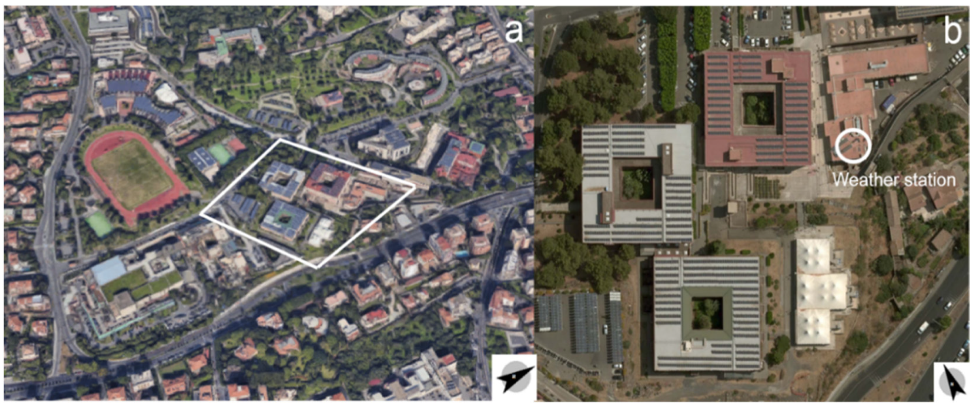
The investigated area is a part of the University Campus of the metropolitan city of Catania along the Mediterranean coast in Southern Italy (latitude 37°30′ North and longitude 15°04′ East). This area was selected for its peculiar urban texture, high population density, as well as urban density.

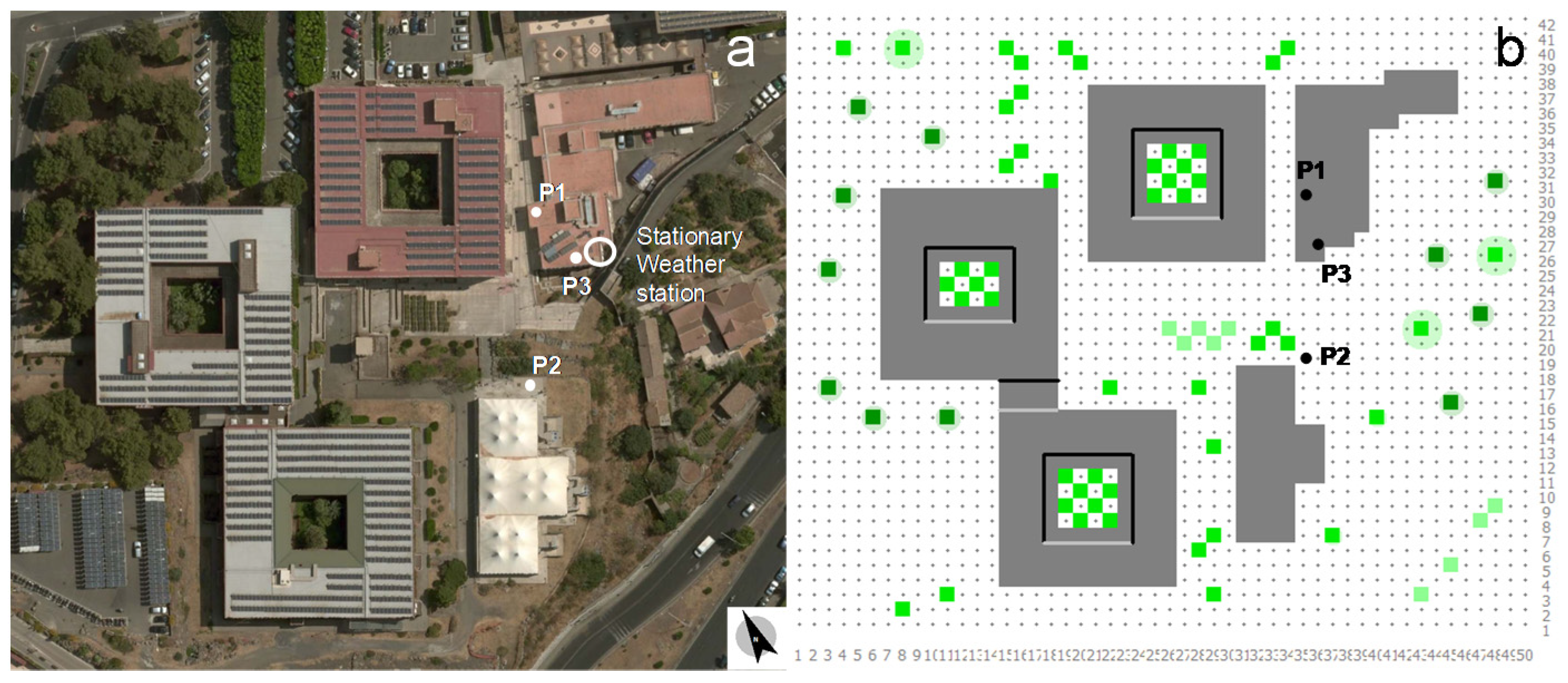
According to the international Köppen–Geiger climate classification, Catania is characterized by warm and humid summer and moderately cool, wet winter. In the summer, the average outdoor temperature ranges from 23 °C to 35 °C, with peaks of 39 °C when hot winds blow from North Africa. Figure 3 shows the investigated area.

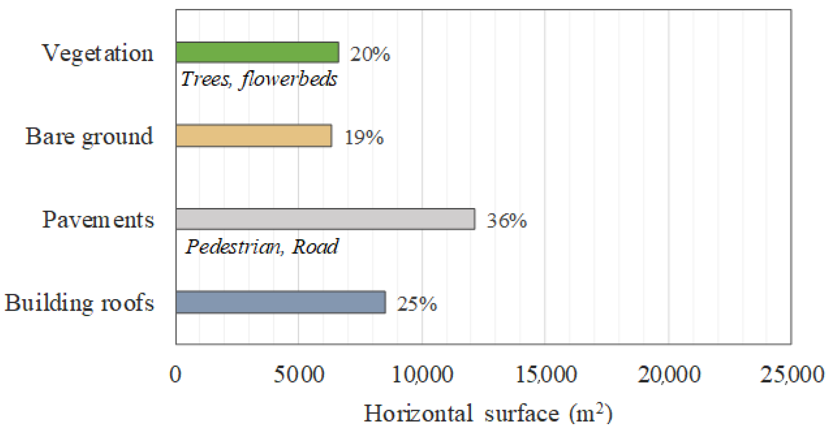
The area has a surface of around 33,600 m² and includes five buildings 5.00 to 15.00 m high that host classrooms and Department offices. The squared buildings have huge sizes (35 × 35 m²), as shown in Figure 3b. Figure 4 shows the different typology of the land surface of the investigated area at current state.

Currently, about 8496 m² are the building roofs and about 12,160 m² is a paved area (pavements, roads), while the presence of vegetation is estimated at around 6610 m² of the total investigated area.

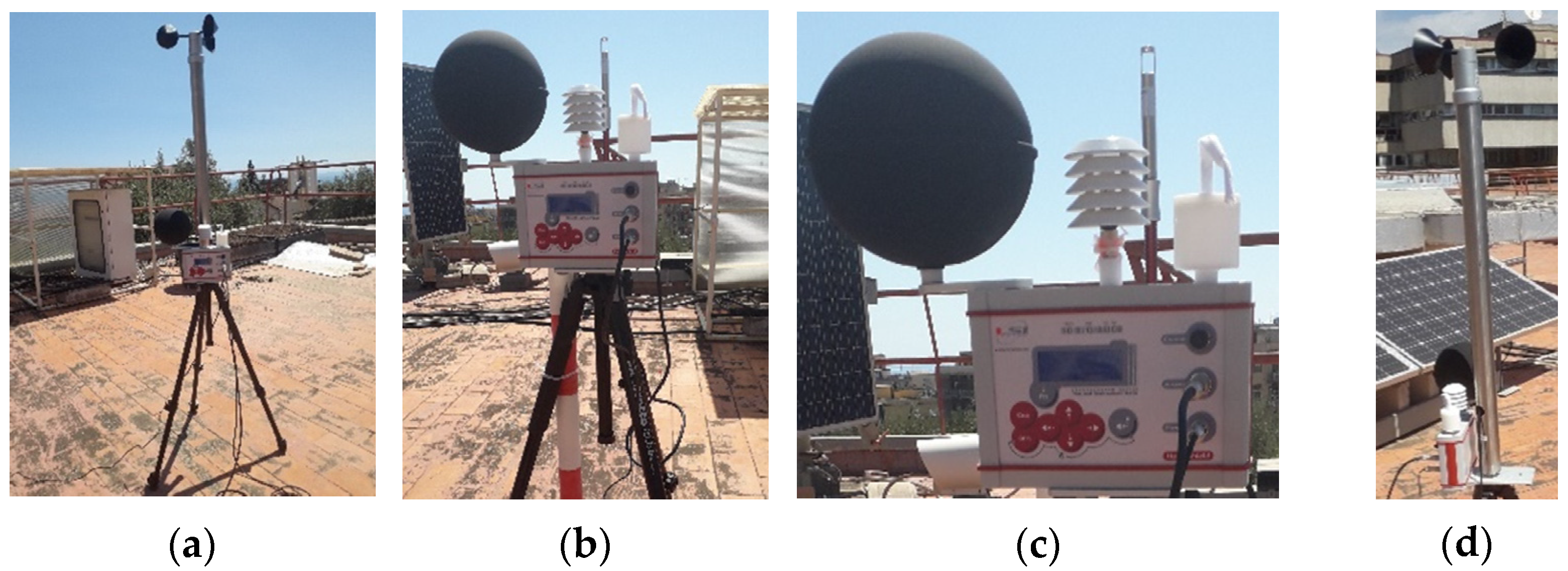
The measurements were taken with a LSI-Lastem weather station (equipped with the air temperature sensor, black globe thermometric sensor, thermo-hygrometric sensor, and anemometer) located on the roof of the building of the Electric, Electronics, and Computer Engineering Department.

3.1. Baseline Scenario

3.1.1. Model Simulation

The simulation model presents a domain with a number of grids equal to 50 × 42 × 30 featured by a mesh of 4.0 × 4.0 × 1.0 m. The total domain dimension is 200.0 × 168.0 × 100.0 m. The height along the z-axis of the domain is constant until 15.0 m, which represents the size of the tallest building; after that, it increases with a telescopic factor rate of 10%. Along all borders of the domain, six cells of nesting grids are set. The time step of the simulation was constant and equal to two seconds to avoid numerical instability and convergence issues.

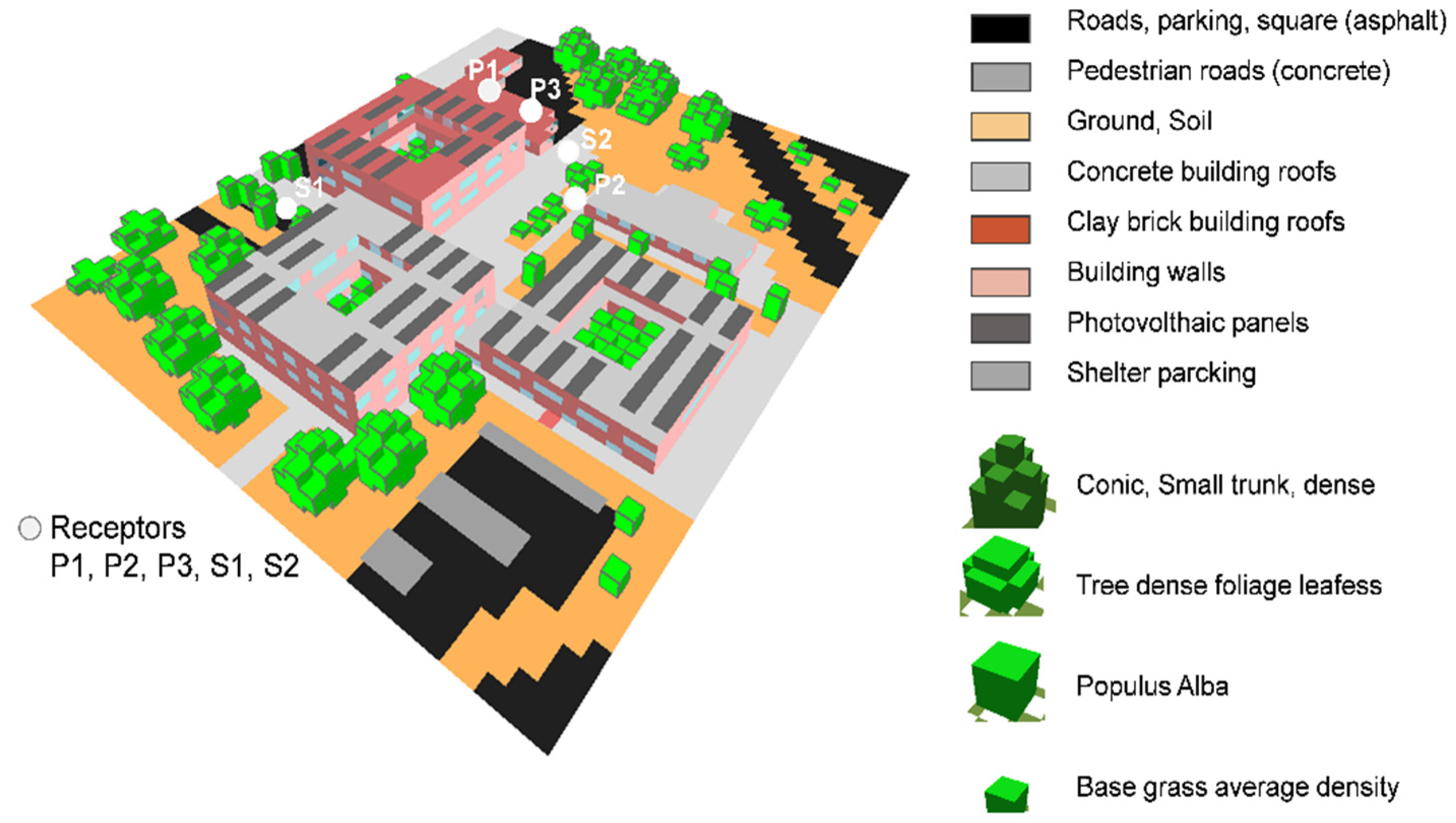
Figure 5 displays the 3D Model of the investigated area in the baseline scenario where green color represents the vegetated area (trees or shrubs), black color represents the paved area (road, parking, square), dark gray represents photovoltaic panels, light gray represents pedestrians’ roads, and light brown represents the unpaved area (ground, soil).

In the domain, three receptors, namely P1, P2, and P3, have been selected for the purpose of validating the CFD model (see Figure 6).

In the same way, two receptors (S1 and S2) have been selected to investigate locally the variation of microclimate and thermal comfort under the three proposed different scenarios (see Figure 5).

Two sequences of simulations were carried out: from 6.00 a.m. on July 28 to 6.00 a.m. on July 31 and from 6.00 a.m. on August 22 to 6.00 a.m. on August 25. The simulations started at sunrise when the energy balance is almost equal to zero.

Finally, the parameters for calculating PMV and PET were set up as follows: age of users, 24 years old, medium height of 1.70 m, average weight of 70 kg, metabolic rate equal to 1.50 Met, and clothing thermal insulation (clo) equal to 0.50.

3.1.2. Materials and Thermo-Physical Properties

Materials and thermo-physical properties have been modeled according to international literature sources [12]. The outer surfaces of buildings, roads, pedestrian pavements, and other outdoor spaces are made up of “standard” materials that absorb remarkable solar radiation during daytime contributing to the release of high heat flux.

Globally, eight different kinds of urban surfaces have been identified and defined. Aiming to simplify the model, for each of them, a single value of albedo and emittance based on the material predominance was assigned.

Table 3. Thermal and optical properties of existing material.

Urban Components	Albedo (ρ)	Solar Emittance (ε)
Roads, parking, square (asphalt)	0.20	0.85
Pedestrian roads	0.30	0.85
Ground, soil	0.20	0.95
Concrete building roofs	0.30	0.90
Clay brick building roofs	0.30	0.90
Building walls	0.20	0.90
Photovoltaic panels	0.625	0.90
Shelter parking	0.20	0.90

reports the values of albedo and solar emittance adopted for the model.

It is worth highlighting that PV systems are installed on many roofs. Consequently, they have been modeled too. Indeed, they have been considered as conventional roofs with a reduction in reflectivity of around 0.625. The latter was calculated considering the conversion rate of the solar radiation into electricity (15%), the PV panel reflection (10%), and the portion of absorbed energy that comes back to the external environment by convection and radiation from the upper and lower surface of the PV modules (12.5%).

The vegetation occupies about 20% of the total land area in the model. Indeed, most trees and shrubs are placed to the north-west of the selected area, whereas the extensive vegetation and bare ground are facing south-east. The trees are predominantly conifers, but some deciduous plants are present, while flowerbeds are occupied by some small grass and evergreen plants. The plants identified on the area and simulated are conic: small trunk, sparse, medium 15 m (conifer); tree: 10.0 m height, dense foliage, leafless (conifer); and Populus Alba: 7.0 m height (deciduous) and base grass, average density, 0.50 m tall. All the plants are characterized by the albedo estimated in the range 0.25–0.40.

Thermo-physical and optical properties of plants as well as the leaf area density (LAD) are reported in

Table 4. Thermo-physical and optical properties of plants included in the model.

Type	Species	Height (m)	LAD (-)	ρ (-)	ε (-)
Conic, small trunk, dense	conifer	15.0	2.3	0.12	0.10
Tree dense foliage leafless	conifer	10.0	2.5	0.25	0.12
Populus alba	deciduous	7.0	2.0	0.40	0.20
Base grass, average density	-	0.30	0.30	0.25	0.15

.

3.2. On Site Weather Measurements

Figure 6 shows the actual locations where the portable weather stations have been placed during the field measurement and surveys.

Table 5. Locations and investigated periods selected for measurements survey.

No	Locations	Time Periods	Locations	Height a.g.l. (m)
1	P1	10.00 a.m. on July 29–6.00 p.m. on July 30	Roof Terrace of building. n. 13	5.4
2	P2	10.00 a.m.–6.00 pm. on July 30	Pavements	7.0
3	P3	12.00 a.m. on August 22–12.00 a.m. on August 24	Roof Terrace of building. n. 13	5.4

reports the locations and time periods of the survey.

The portable station was settled at 1.2 m on the roof of the building n. 13 (P1 point) from 10.00 a.m. on July 29 to 6.00 p.m. on July 30 and in P3 point in close proximity to the stationary weather station from 12.00 a.m. on August 22 to 12.00 p.m. on August 24 (Figure 6a). The mobile station was installed on a tripod of 1.2 m height and placed close to the building n. 15 (P2 point) from 10.00 a.m. on July 30 to 6.00 p.m. on July 30.

4. Calibration and Validation

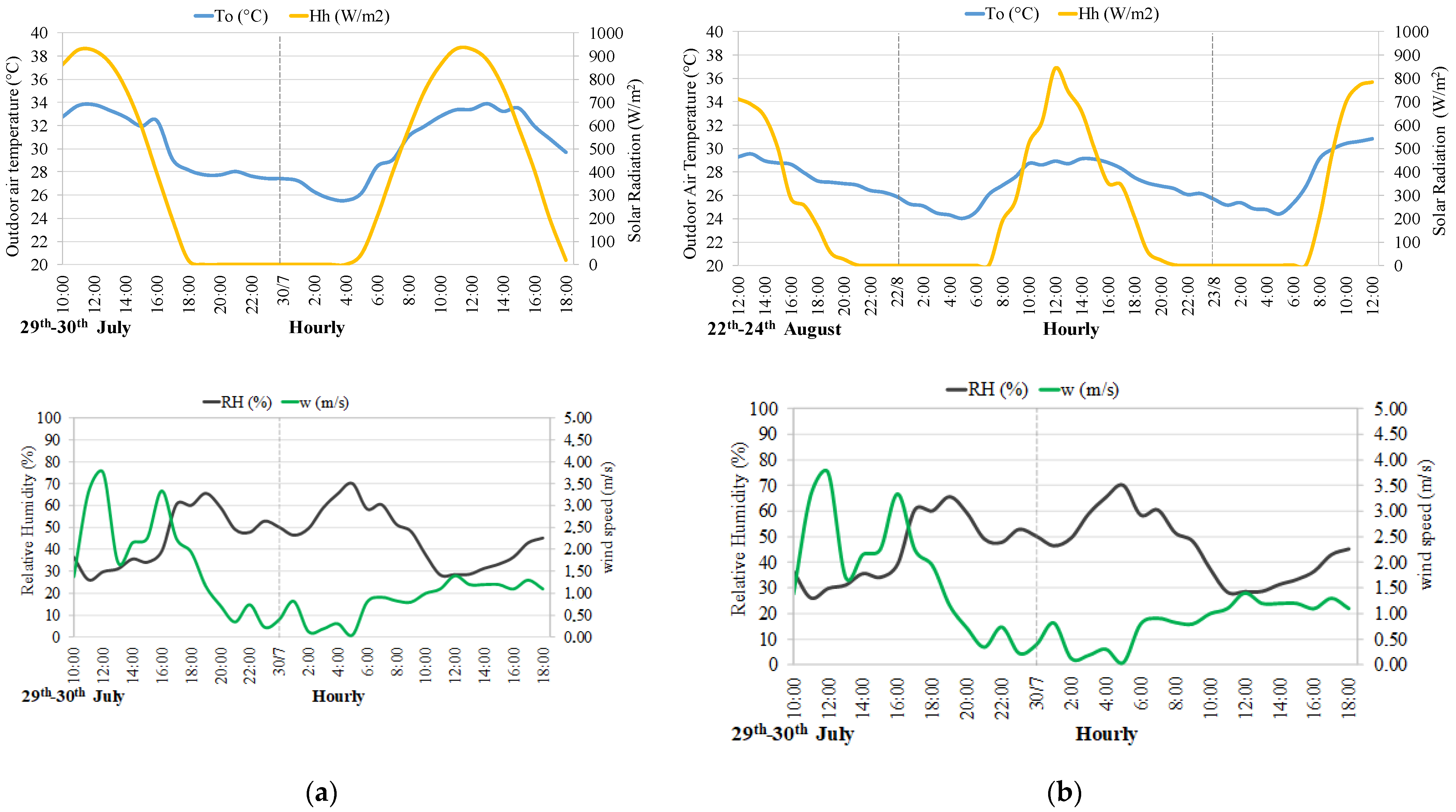
The simulation model was calibrated using hourly data of weather station reported in Figure 7.

The reliability of the ENVI-met model was evaluated against the statistical indicators introduced in Section 2.4 using the data recorded by the portable weather station in P1, P2, and P3.

Table 6. Validation indices of the ENVI-met model.

Variables	Statistical Indices	Unit		Locations
			P1 (h = 5.41 m) 29th–30th July	P2 (h = 1.20 m) 30th July	P3 (h = 1.20 m) 22th–24th August
To	MAE	°C	1.33	2.41	0.82
	RMSE	°C	1.60	2.50	0.69
	r	-	0.96	0.95	0.98
	R2	-	0.93	0.91	0.94
RH	MAE	%	4.76	4.95	3.04
	RMSE	%	5.49	6.02	2.15
	r	-	0.94	0.77	0.97
	R2	-	0.88	0.60	0.95

reports the calculated statistical indicators.

The analysis of MAE and RMSE values for the air temperature and relative humidity reveal a not perfect correlation at the points P1 and P2, while at P3 the discrepancies are quite low. For the air temperatures, MAE at P3 is less of 1.0 °C, while anywhere else it exceeds 1.0 °C, and it is even above 2.0 °C at P2.

Nevertheless, a good correlation with experimental measurements is confirmed in terms of air temperature by the high values of the correlation coefficient “r“ and of the determination coefficient R², which are always higher than 0.90. Although the statistical indicators do not achieve optimal values, the profiles of air temperature and relative humidity are very close and similar in all points.

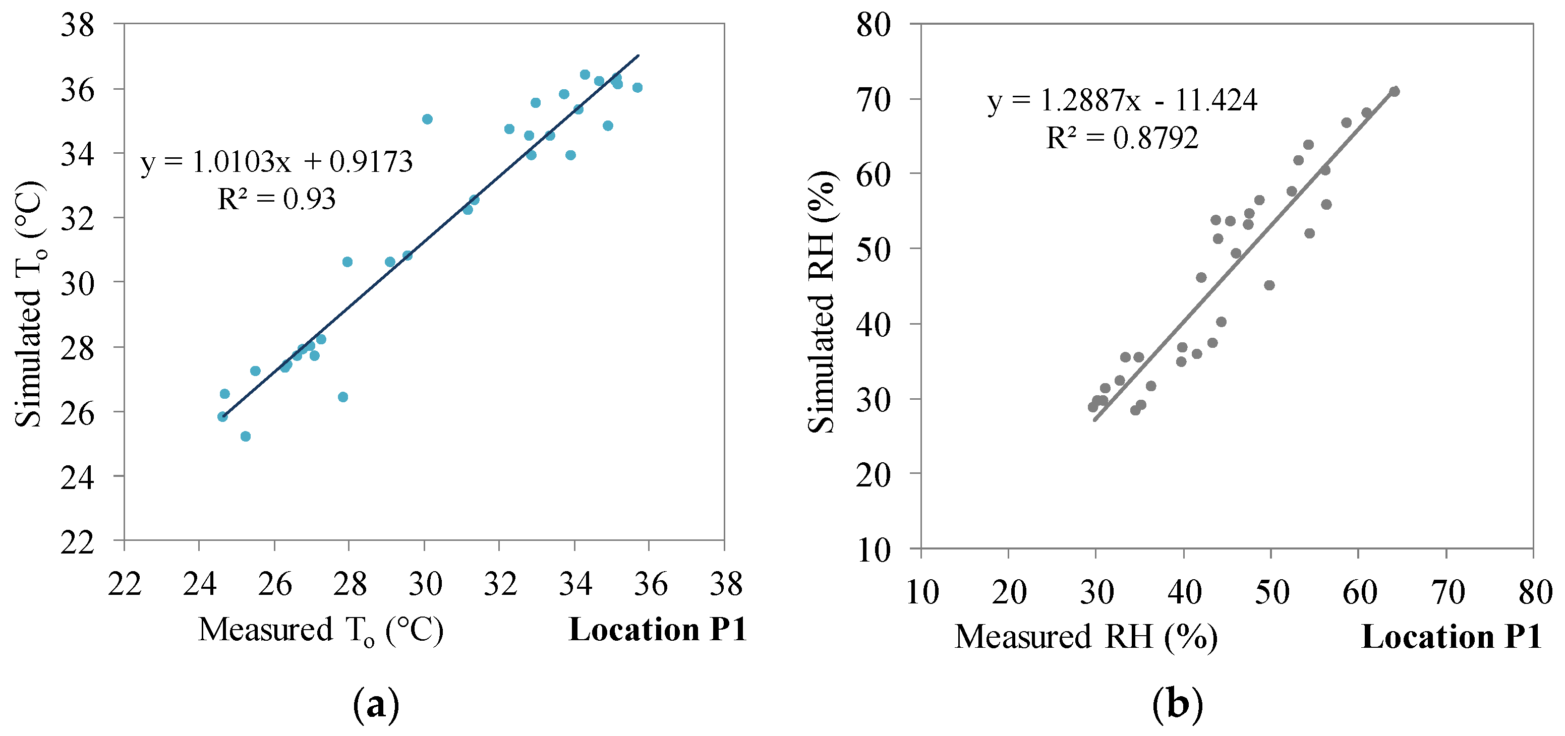
Indeed, as an example, the comparison between the measured and simulated values at P1, displayed in Figure 8a,b, highlight a good correlation for air temperature (T_o) and relative humidity (RH).

Nevertheless, during the night, the temperatures simulated are around 1.0 °C lower compared with the measured ones. This could be due to an overestimation of the low long-wave radiation exchange with the sky because of low sky temperatures or high values of emittance of the outer layer of the building’s surface. Despite this, the model does not seem to be affected by the fraction of anthropogenic heat that actually contributes to climate microscale.

During the hours of maximum solar radiation, the profile of simulated air temperature is lower than about 1.0–2.0 °C with respect to that measured trend. A similar result was also found in other studies [45]. For example, Mohamed et al. [46] have evaluated the microclimate of an urban area located within the Islamic Quarter of Cairo (Egypt). They have compared ENVI-met and measured data, discovering a difference in peak value of the temperature of 2.0 °C between 11.00 a.m. and 3.00 p.m. on a summer day.

Gusson and Duarte performed on-site microclimate measurements for the calibration of ENVI-met models of two densely populated districts in São Paulo in Brasil (Brasilândia and Bela Vista). A grid with a mesh of 3 × 3 × 3 m³ was adopted for modeling both districts in ENVI-met. Despite good correlation coefficients, they found out a difference in peak value of temperatures of 3.2 °C between simulated and recorded data at around 12 p.m. [47].

5. Proposed Scenarios

Three scenarios were proposed and evaluated to enhance outdoor environmental microclimate conditions:

• Cool scenario (Cs), in which a reflective paint is applied on the pedestrian pavements, roads, and building roofs;
• Green Roof scenario (GRs), in which extensive green roofs are installed with an increase of surface cover at around 25%;
• Green Saturation scenario (GSs), in which any available area is covered with vegetation and green roofs. In this way, the green surface cover increases by around 44%.

More in detail, the Cool scenario (Cs) consists in the replacement of conventional materials with cool paints for pedestrian roads, pavements roads, and the application of cool paint on the roofs of all buildings. The cool materials are supposed to have high albedo and high emissivity to reflect the solar radiation. Commercial products were adopted: their thermal and optical features are reported in

Table 7. Surface cover (%) treated with cool materials.

Urban Components	Surface (m2)	Surfaces Ratio (%)	Albedo (ρ)	Emittance (ε)
Cool pavements	12,160	36%	0.80	0.90
Cool roofs	8500	25%	0.80	0.90
Total	20,650	61%	-	-

[48].

The total surface treated with cool materials is 20,650 m², which represents 61% of the investigated area. The Green Roof scenario (GRs) is based on the installation of 8500 m² extensive green roofs on the top of all buildings. The features of the substrate and vegetation layer of the green roof are reported in

Table 8. Features of the substrate layer.

Height	H	0.15	m
Thermal conductivity	λ	1.00	W·m−1·K−1
Absorptance	α	0.60	-
Albedo	ρ	0.30	-
Emittance	ε	0.90	-
Moisture content	Θsat	0.50	m−3·m−3

and

Table 9. Features of the vegetation layer.

Height	H	0.30	m
Leaf Area Index	LAI	1.50	m2·m−2
Absorptance	α	0.60	-
Albedo	ρ	0.25	-
Emittance	ε	0.95	-
Transmissivity	τ	0.15	-

, respectively.

Data available in the scientific literature [49] were considered for the thermo-physical properties of substrate and vegetation layers. The Green Saturation scenario (GSs), in addition to the green roofs, considers the planting of new trees, such as Populus alba and pine, with an average height of 10 m, and new grass until it reaches the saturation of bare soil. Pines and Populus alba have been adopted, because they are endemic species and have physical characteristics that are suitable for urban greening. The surface of vegetation is 14,800 m² in the green saturation scenario.

6. Results and Discussion

6.1. Microclimate and Thermal Comfort Daily Variation

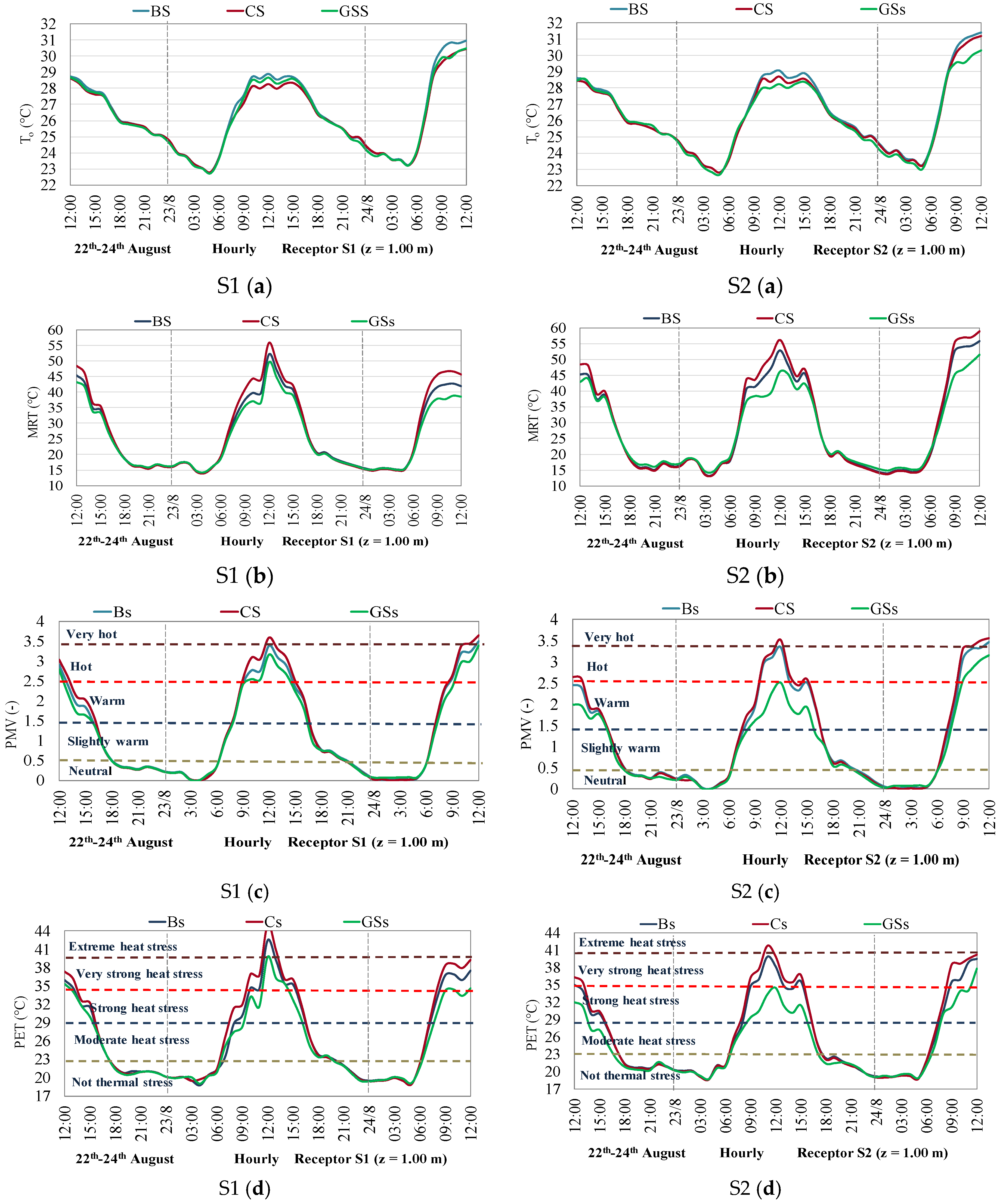
This section reports the results of thermal comfort simulation for the Baseline, Cool, and Green scenarios. An accurate analysis has highlighted that Green Roofs (GRs) do not affect the microclimate at pedestrian level. For this reason, Figure 9a–d reports only the profile of air temperature, mean radiant temperature, predicted mean vote and physiological Equivalent Temperature for the Baseline (Bs), Cool (Cs), and Green Saturation (GSs) scenarios at the S1 and S2 receptors.

Under the Baseline scenario (Bs), the air temperature ranges from 22.8 °C to 31.0 °C for both S1 and S2 receptors. At noon, the Cool scenario (Cs), compared to the baseline scenario (Bs), gives place to a decrease of the air temperature by 0.5 °C at the S2 receptor and by 0.8 °C at the S1 receptor.

The Green Saturation scenario (GSs) shows the best performance at the receptors S2, which is close to green spaces, with a reduction in the air temperature of about 0.8 °C. Nevertheless, a decrease in the air temperature is also achieved at the receptor S1, which is quite far from green areas.

It is to outline that during the daytime the Cool scenario (Cs) shows values of MRT higher than in the green saturation (GSs) and baseline (Bs) scenarios; this happens for the zone closest to the building facades due to highest albedo of these surfaces. An increase of 4.0 °C is observed at S2 receptor and of 3.4 °C at S1 receptor.

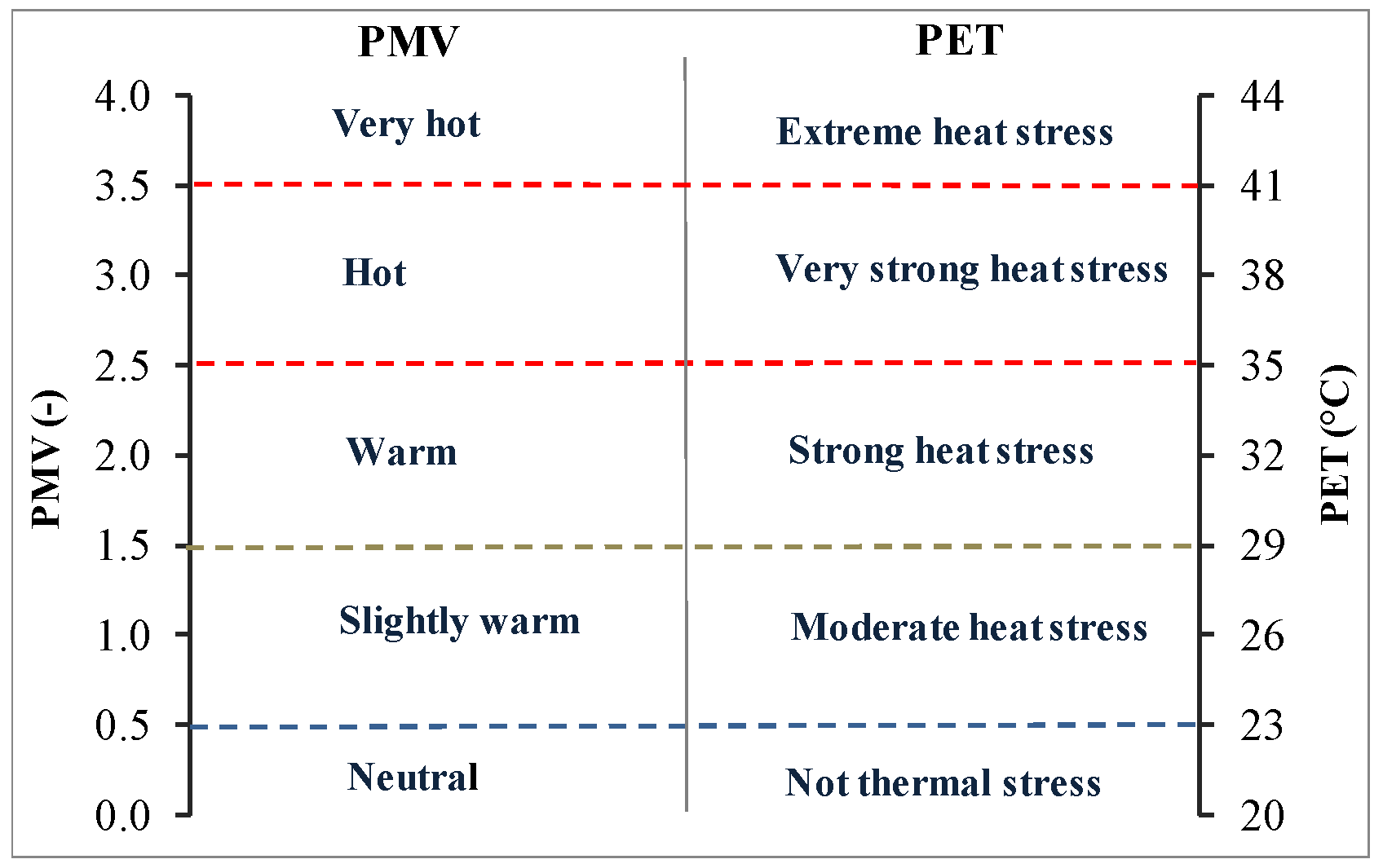
As to the PMV, a value of 2.5 is exceeded for all scenarios for both receptors from 8:00 a.m. to 4.00 p.m. The only exception is observed at the receptor S2 for the Green Saturation scenario (GSs). A similar result is observed for the PET index, which is higher than 35.0 °C, “very strong heat stress”, excepting at the receptor S2 for the Green Saturation scenario (GSs).

However, during the hour of maximum solar radiation, the highest values of PMV and PET, according to the value of MRT, have been observed for the Cool scenario. It has to be highlighted that the trend of all investigated parameters show a rapid drop of the curve at around 2.00 p.m. on August 23 due to a decrease of direct solar radiation caused by clouds. In any case, the best results are achieved by the GSs, for which the PET ranges from 19.9 °C to 36.4 °C.

The cumulative frequency distribution was also calculated for the following parameters: T_o, MRT, PMV, and PET during the selected period from 12.00 p.m. on August 22 to 12.00 p.m. on August 24.

Actually, Figure 10a–d reports only the cumulative frequency distribution of air temperature and mean radiant temperature of the Baseline (Bs), Cool (Cs), and Green Saturation (GSs) scenarios in the S1 and S2 receptors.

It can be seen that in the Cool scenario (Cs), the air temperature T_o exceeds 28 °C for 10% of the time. The situation is thus better than in the Baseline scenario (Bs), where T_o exceeds 28 °C for about 30% of the time. That may be explained on the basis of the previous remarks.

From Figure 10b, it is evident that the three scenarios are better differentiated in terms of MRT, especially for MRT higher than 33 °C. As to the parameters more strictly related to thermal comfort (PMV end PET), it can be seen from Figure 10c that all investigated scenarios reach the “Warm” level. Actually, the “warm level” is exceeded 25% of time in the (Cs) and 20% in the (Bs). The GSs exceeds for 10% of time the “Warm” category in the receptor S1. The effect of the Green Saturation scenario (GSs) is remarkable in receptor S2.

It worth highlighting that, as far as the PMV is concerned, the worst results were obtained in the (Cs), while the best performance was achieved by the GSs. This trend is even more evident in the cumulative frequency distribution of PET.

6.2. Spatial Analysis

6.2.1. Air Temperature, Wind Speed, and Relative Humidity

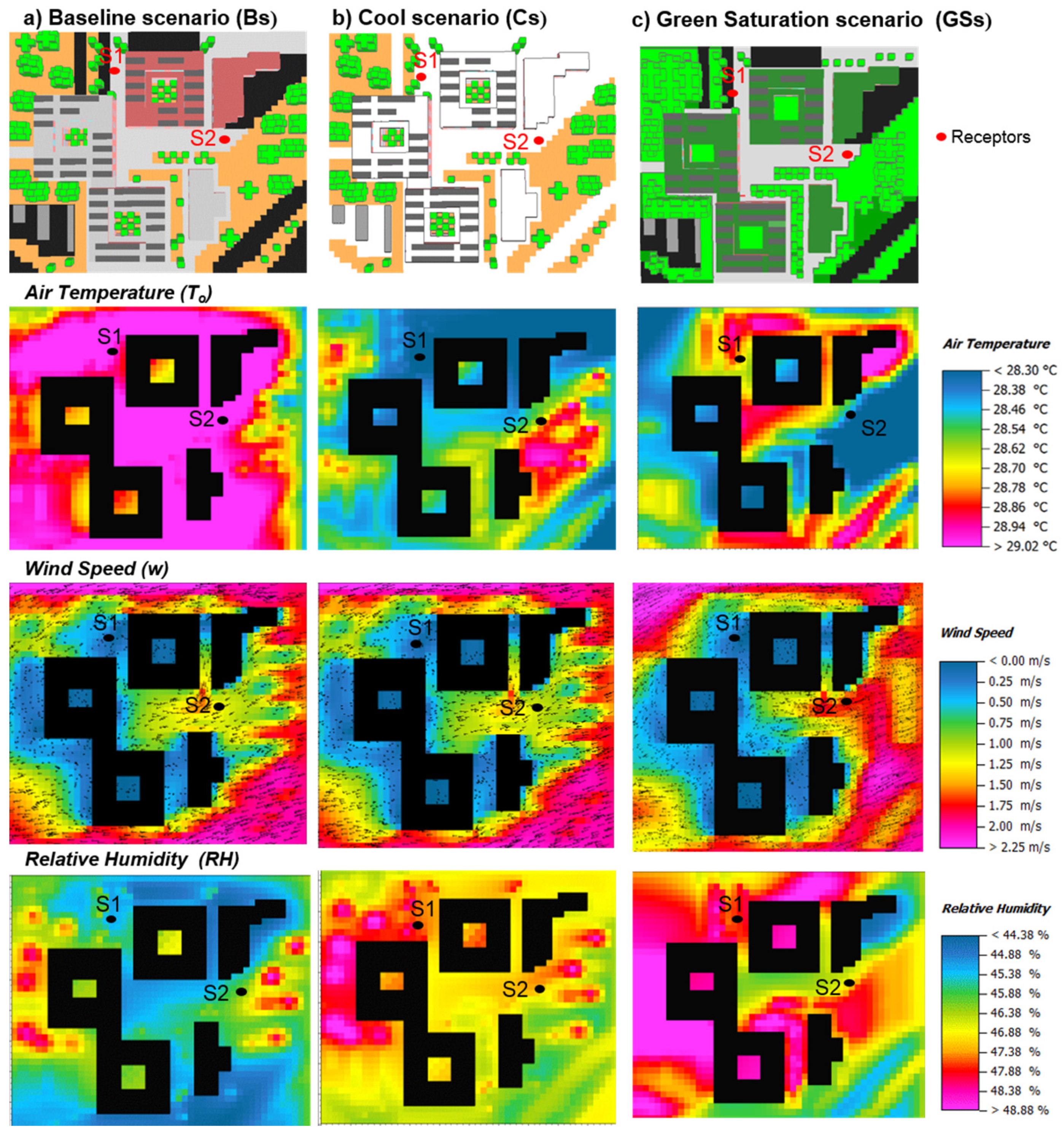
Figure 11 collects a horizontal view (x-y) of air temperature, wind speed, and relative humidity for the three scenarios at 1.00 m height above the ground level at 12:00 am on August 23.

In this section, the scenarios are analyzed according to a spatial point of view, considering the following parameters: air temperature (T_o), wind speed (w), and relative humidity (RH). In the Baseline scenario (Bs), the air temperature of 30.0 °C is reached in most of the areas analyzed.

The highest values of air temperature occur on waterproof surfaces, such as pedestrian pavement and roads, while the minimum value of temperature, of about 28.4 °C, occurs on unpaved surfaces. Under the Cool scenario (Cs), temperatures lower than 29.0 °C have been found in all the investigated areas.

Above soil surfaces, the temperatures range between 28.5 to 28.8 °C and over the roads and pedestrian pavements, the temperature is about 28.2 °C. Globally, cool pavements and roofs allow to reduce the peaks of about 1.0 °C.

For the Green Saturation scenario (GSs), the maximum external air temperature is 29.2 °C, whereas the minimum is 28.0 °C. Consequently, this latest scenario is the most effective, especially regarding the magnitude of minimum values of air temperature.

However, it is worth noticing that the cooling effect of vegetation is not limited to spaces where the plants were added, but their effects are spread to all the surrounding areas.

As regards the field of wind, it is possible to observe that the wind comes from the east, and its speed ranges from 0 to 2.25 m/s. As predicted, the highest wind speed is observed in open areas, whereas areas of stagnation appear behind the buildings or in the narrow spaces between the buildings. Moreover, in areas where vegetation is most present, substantial disturbances of wind speed occur as a consequence of the highest roughness of the soil surface.

The maps of relative humidity, for the three scenarios, indicate that the areas where vegetation is present are characterized by the highest relative humidity (up to 49%). In the Green Saturation scenario (GSs), the highest values of relative humidity were found. A maximum value of 51.6% was recorded in areas where the vegetation is very dense.

6.2.2. Soil Temperature, Mean Radiant Temperature, and Thermal Comfort Indexes

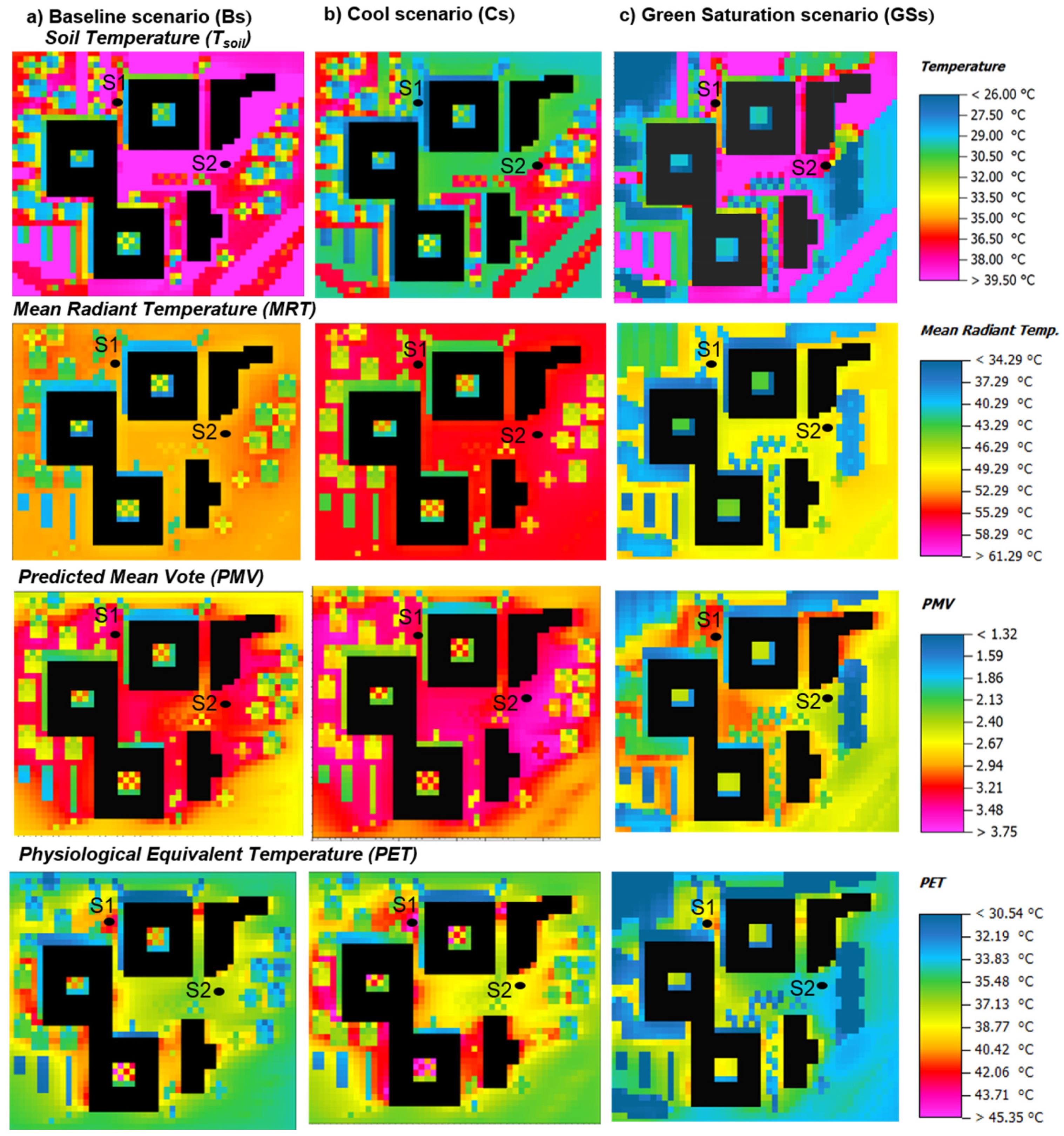
In this section, the scenarios are analyzed by a spatial point of view considering the following parameters: soil temperature (T_soil), mean radiant temperature (MRT), predicted mean vote (PMV), and physiological equivalent temperature (PET) (Figure 12).

For the Baseline scenario (Bs), the soil temperature reaches the maximum values of 44.2 °C in paved areas, while just 27.0 °C is observed in the vegetated or shaded areas. The MRT has an average value of 52.0 °C in the whole area, which drops to 43.0 °C in shaded areas. The PMV index has a maximum value of 3.03 and a minimum value of 1.99.

The areas occupied by pedestrian pavements and roads have PMV values of about 3.00 and can be classified as hot areas, whereas the green areas with PMV values of 2.00 can be classified as warm areas. The PET index has a maximum value of 47.0 °C in paved areas and a minimum of 30.5 °C in the vegetation areas. Therefore, the Baseline scenario can be classified as hot and characterized by rather strong heat stress. Thus, for most of the investigated areas, the environment is very far from comfortable conditions, and high degrees of discomfort are perceived by the people.

The Cool scenario (Cs) shows values of soil temperature between 25.1 °C and 38.8 °C. On the surface of cool pavements, one can observe a reduction at around 5.0 °C compared to the maximum value of the Baseline scenario (Bs) and a reduction by 2.0 °C in the minimum value. It has to be highlighted that the mean radiant temperature reaches values of 55.0 °C almost in the whole area with an increment of about 3.0 °C compared to the Baseline scenario. This quite unexpected outcome depends on the remarkable amount of solar radiation reflected from the cool pavements and able to cause an increase in the temperature of the surrounding surfaces. The PMV ranges from a minimum value of 2.08 to a maximum of 3.50. In the Cool scenario, both the minimum and maximum values of PMV are higher than in the Baseline case. The PET index has a maximum value of 47.6 °C and a minimum value of 31.4 °C, with an increment of about 1.6 °C and 1.0 °C with respect to the Baseline scenario. It is worth to be highlighted that in the areas between neighboring buildings and in the spaces between the cool pavements and buildings is apparently a strong increase of PET. These areas suffer because of high reflected radiation and relative humidity.

Although the surface temperature of the pavements is reduced, the multiple heat reflections lead to an increase of the human thermal stress, as deductible by observing the magnitude of the maximum and minimum values of PMV and PET, compared to the baseline scenario.

Looking at the map of the reflected radiation, it is worth underlining that the cool pavements reflect in the average 200 W/m² against 170 and 130 W/m² of the Baseline (Bs) and Green Saturation (GSs) scenarios, respectively. The previous outcome confirms that the application of cool paint over a paved area contributes to the deterioration of the outdoor thermal comfort due to the increase of the reflected solar irradiance.

Figure 13 reports the 2D maps of reflected solar radiation (Gr) for all investigated scenarios on a horizontal plane at pedestrian level, at 12.00 a.m., on August 23.

The Green Saturation scenario (GSs) offers the best behavior in terms of MRT, PMV, and PET. As a matter of fact, MRT ranges between 34.4 °C and 52.3 °C. In addition, PMV has a minimum value of 1.4 and a maximum value of 3.0. Finally, PET assumes values between 28.0 °C and 41.1 °C.

To further characterize the various scenarios, it is useful to introduce the indicator I_PET defined by the variation of PET between the Baseline (Bs) and the proposed scenarios (P_s,i), as follows:

$${\mathrm{I}}_{\mathrm{PET},\mathrm{i}}(\%)=\frac{{\mathrm{PET}}_{\mathrm{Ps},\mathrm{i}}-{\mathrm{PET}}_{\mathrm{Bs}}}{{\mathrm{PET}}_{\mathrm{Bs}}}$$

(2)

The i index is referred to the different proposed scenarios, i.e., Ps = Cs, Ps = GSs.

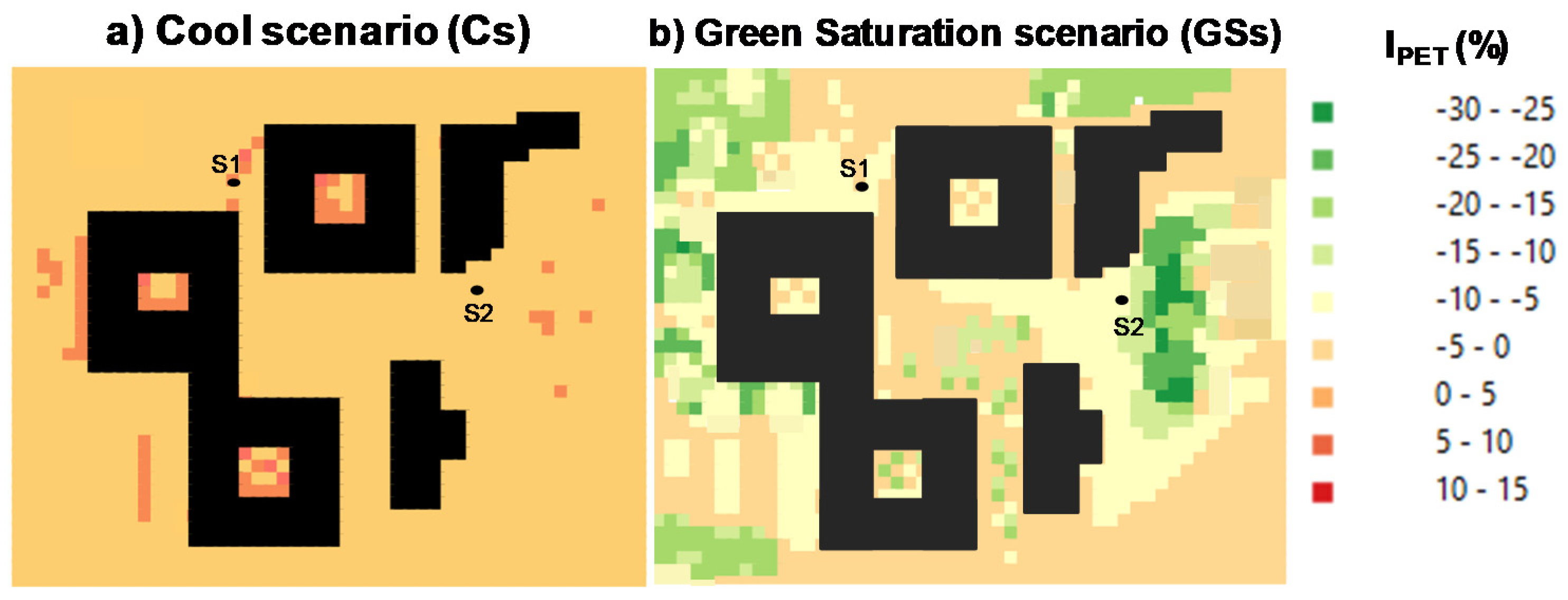
Figure 14 depicts the I_PET for the Cool and Green Saturation scenarios at z = 1.00 m at noon on August 23. The positive sign means an increase of PET, while the negative sign indicated a reduction.

As it is possible to see, the Cool scenario shows an increase in the PET in all points of the investigated area. Figure 14 shows that the highest increase of the PET (10–15%) occurs in the internal courtyards of the buildings, mostly due to the multiple reflections. On the contrary, the Green Saturation scenario shows a reduction in the PET values in all investigated areas.

The highest reduction (−30% to −20%) is reached in the areas with trees and shrubs. It is worth pointing out that a decrease in PET of about 5% is achieved even in areas not provided with vegetation.

Of course, the beneficial effect of the Green scenario has to be attributed to the evapotranspiration of plants, which leads to a cooling effect in the surroundings. Moreover, the shading effect of trees and shrubs allows the creation of small areas where the warming sensation is attenuated.

Generally, under the Green Saturation scenario, it is possible to achieve acceptable outdoor thermal comfort with the exception of very limited areas represented by the surfaces between neighboring buildings and spaces around the buildings.

6.2.3. Spatial Cumulative Frequency Distribution

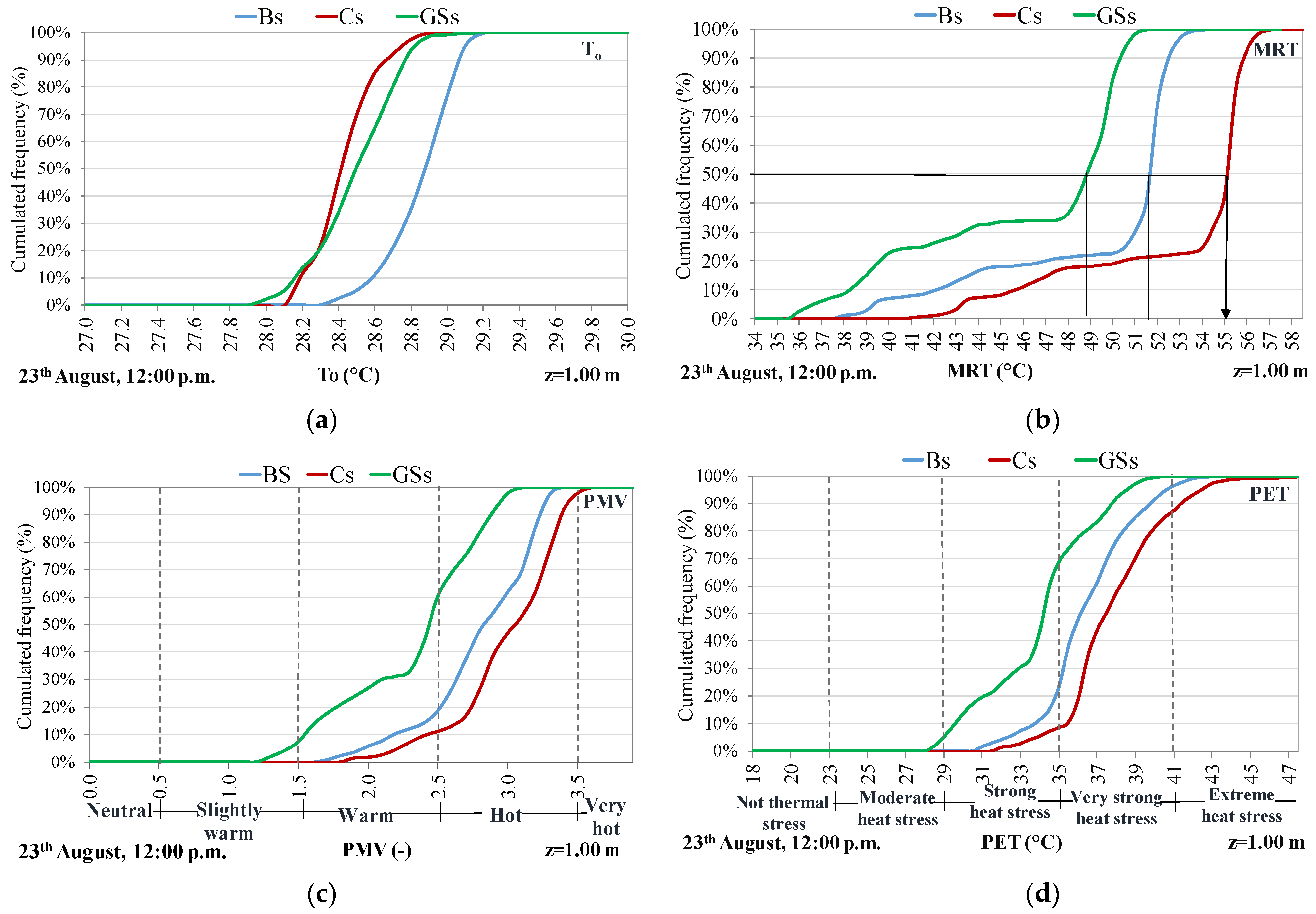
Figure 15 shows the cumulative frequency distribution of T_o, MRT, PMV, and PET for Baseline (Bs), Cool (Cs), and Green Saturation (GSs) scenarios with reference to the whole investigated area at height of 1.0 m above the ground level at 12.00 p.m. on August 23.

Overall, the graphs show that in spite of the fact that the Cool scenario (Cs) exhibits the best performance in terms of T_o, it proves to be the worst case in terms of MRT, because of the high reflectivity assumed by the surfaces treated with cooling paints.

The consequences can be seen in the PMV and PET, considering that both PMV and PET are more sensitive to MRT than to T_o.

This is a clear hint about the adverse effect that reflective paints may cause on the thermal sensation in the outdoor environment. In conclusion, compared to the baseline scenario, the best performance thus pertains to the GSs.

6.3. Spatial Averages

In order to provide a synthetic comparison of the three proposed scenarios, the average values of the thermal parameters and the comfort Indicators were calculated. The spatial average values on the whole area relating to air temperature, mean radiant temperature, relative humidity, predicted mean vote, and physiological equivalent temperature is as follows:

$$\overline{\mathrm{L}}=\frac{{\displaystyle {\sum }_{\mathrm{i}=1}^{\mathrm{n}}{\mathrm{L}}_{\mathrm{n}}}}{\mathrm{n}}$$

(3)

Here, $\overline{\mathrm{L}}$ is the average spatial value of any previously mentioned (L) parameter extended to all cells (n) of the domain.

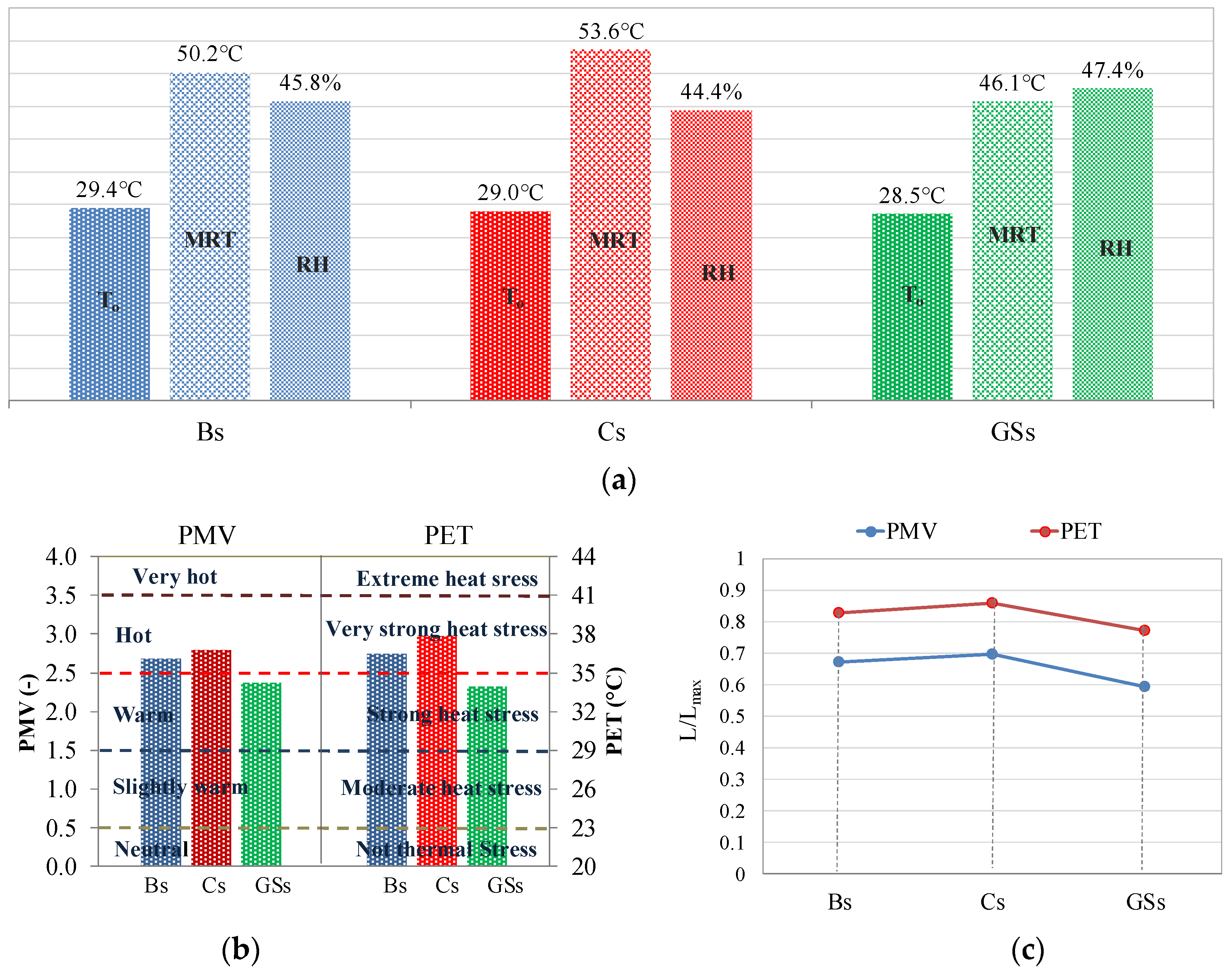
The average values of the investigated parameters for each scenario are compared and reported in Figure 16. In particular, Figure 16a displays a comparison in terms of outdoor air temperature, mean radiant temperature, and relative humidity. Figure 16b reports the comparison in terms of the mean values of PMV and PET according to the thermal sensation scale and heat stress categories. All the microclimate parameters and thermal comfort indicators refer to 1.00 m above the ground level and at 12.00 a.m. on August 23. Finally, PMV and PET normalized to their maximum values for the three analyzed scenarios are reported in Figure 16c.

Again, overall, Figure 16 shows that the best results are achieved by the Green Saturation scenario (GSs), which has the lowest of value T_o, MRT, PMV, and PET. These results are attributable to the synergic effect of shading and evapotranspiration processes. On the other hand, the Cool scenario (Cs) has the worst performance even with respect to the Baseline scenario (Bs), for all the mentioned parameters, with the exception of T_o.

It is to outline, that although the surfaces treated with green materials are less by 17% than those treated with cool materials, they allow achieving the greatest benefits for the urban microclimate and thermal comfort at the pedestrian level.

7. Conclusions

This paper aims to identify the effectiveness of urban greening and cool materials as strategies for the enhancement of urban micro-climate and well-being conditions of pedestrians. To this purpose, a micro-scale analysis, based on a numerical model and experimental field measurements, was carried out in the University Campus of the metropolitan city of Catania. The influence of materials and vegetation was analyzed to assess pedestrian comfort in different scenarios. The outcomes of the simulations reveal that the green roof does not affect the microclimate at the pedestrian level, while the application of cool materials can reduce the air temperature by almost 1.0 °C in the peak value compared to the other scenarios, while it is the Green Saturation scenario that ensured the best performance in terms of MRT, PMV, and PET.

Other meaningful results were also provided by the cumulative frequency curves. They allowed the estimation of how long a given condition of T_o, MRT, PMV, or PET is holding, and showed that the three scenarios are more sensitive to MRT than to T_o. Finally, the evaluation of PET and PMV provided comparable results. All the gathered information made it easy to assess the effectiveness of the various mitigation measures.

In conclusion, the methodology used here may be useful to urban planners and policymakers searching for the optimal urban greening and cooling strategies in the urban environment.