Abstract
Precision agriculture aims to use minimal inputs to generate maximal yields by managing the plant and its environment at a discrete instead of a field level. This new farming methodology requires localized field data including topological terrain attributes, which influence irrigation, field moisture, nutrient runoff, soil compaction, and traction and stability for traversing agriculture machines. Existing research studies have used different sensors, such as distance sensors and cameras, to collect topological information, which may be constrained by energy cost, performance, price, etc. This study proposed a low-cost method to perform farmland topological analytics using sensor implementation and data processing. Inertial measurement unit sensors, which are widely used in automated vehicle study, and a camera are set up on a robot vehicle. Then experiments are conducted under indoor simulated environments that include five common topographies that would be encountered on farms, combined with validation experiments in a real-world field. A data fusion approach was developed and implemented to track robot vehicle movements, monitor the surrounding environment, and finally recognize the topography type in real time. The resulting method was able to clearly recognize topography changes. This low-cost and easy-mount method will be able to augment and calibrate existing mapping algorithms with multidimensional information. Practically, it can also achieve immediate improvement for the operation and path planning of large agricultural machines.
1. Introduction
Maintaining adequate food supply has become challenging due to worldwide population expansion and climate change [1,2]. With the advancement of technologies, such as sensors, image processing techniques, and computing capability, precision agriculture has been promoted. Precision agriculture aims to use minimal inputs to generate maximal yields by taking into account the crop’s local field environment.
Precision agriculture includes precise irrigation quantity, correct and appropriate application of chemicals, and weeding, for which the topological characteristics of the crop field are a key component that needs to be considered. For instance, the quantity of irrigation varies drastically due to the change of terrain slopes. Hussnain et al. [3] described that low areas of the crop field are likely to collect more water from either the irrigation or rainfall, meaning that irrigation for those areas should be less compared to that for other areas with high slopes. Mareels et al. [4] concluded that precision agriculture especially for the irrigation system relies heavily on the topological characteristics of the crop field.
Topological terrain attributes also influence the efficiency of implementing large agriculture machines. Machine and tractor fleets used in agriculture improve the efficiency of the farming process, while they also require appropriate terrain attributes to be able to perform and maneuver [5]. Without information about the specific topological characteristics of the field, large farming tractors and implements could become stuck in the field or create unnecessary field ruts. Therefore, information collection for detailed topological characteristics is essential in precision agriculture. This need will only be heightened as farming transitions to autonomous vehicles.
Advanced sensors and computer vision techniques provide an opportunity to collect the topological characteristics from the environment required by precision agriculture. Sensors are becoming smaller and more powerful [6]. In addition, the costs of sensors are decreased, enabling their widespread deployment in practice. The development of computer vision technique has reached the level at which users can efficiently process collected data for decision-making.
However, collecting all information from the crop field not only increases the burden of memory needed by the equipment but also adds more useless information required to be proceeded by the researchers. A method to extract critical and useful information from the field is needed. We propose a method that combines the advanced sensors and inertial measurement units (IMUs) as well as the algorithm to monitor the crop field in real time at a low cost and in a practical manner. In addition, the automated monitor system also performs a field analysis of the relationship between the topological characteristics and crop growth to provide useful information for farmers to adjust their crop management strategies accordingly and in a timely manner.
Thermal remoting sensing is another commonly used technique in this field. Different from optical remoting sensing on the basis of reflected radiation, thermal remoting sensing relies on the emitted radiation of the target objects [7]. It allows the farmers to collect information such as temperature, crop stress, and crop diseases [8,9,10] so the corresponding activities could be performed timely and accordingly.
Unmanned airborne vehicles (UAVs) has been extensively implemented in modern agriculture due to their light weights and low costs, combined with remote sensing technologies. Honkavaara et al. [11] integrated UAVs and remoting sensing techniques to realize consistent data collection and processing for wheat production. Costa et al. [12] implemented UAVs and wireless sensor network to detect crop diseases and applied pesticide, significantly minimizing the amount of pesticide inputs. Maes and Steppe [13] combined thermal remoting sensing and UVAs for crop weed detection and achieved favorable results.
However, in addition to the above remoting sensing and 3D maps that researchers build based on cameras [14], additional information such as the landform and more accurate topography is still a requisite. The terrain will not only affect the growth of plants but also the management process by robot farmers. For example, it significantly increases the processing time and fuel cost for a large machine if there are a lot of turns, and an unbalanced landform could result in different soil and water conservation. Moreover, the algorithms for map maintenance [15] are susceptible to adverse surface conditions, such as unexpected pits, washouts from precipitation, steep slopes, or barriers. These drawbacks can limit the ability of autonomous mapping and further lead to the failure of localization. As a result, high-quality map building is challenging when attempting to include all these details [16]. Moreover, different landforms may result in various growing statuses [17], for example, steep slopes have a higher chance of causing severe erosion processes.
Energy costs associated with sensors constrain their applications. Traditional sensors, such as stereo vision cameras or LiDAR, can provide accurate prediction of the images collected from the fields, but their high power consumptions are too high to be implemented for the needs of large farmland (hundreds and thousands of acres) monitoring. Differently, the IMU sensor is a perfect substitute to be deployed in large farmland monitoring with a tradeoff between performance and energy costs. Table 1 lists the power consumption and market price for different types of sensors, showing that IMU sensors have advantages over other types of sensors with super low energy consumption and market price.

Table 1.
Power consumption and market price of different types of sensors.
To solve these problems, we propose an approach that addresses the proper hardware implementation and associate algorithms for the sensors data as shown in Figure 1. This work aims to augment the dimensional information of the existing farm mapping system. The hardware implementation includes the sensors’ selection, application, and configuration. We build upon this hardware with a customized data fusion algorithm to process the collected data.
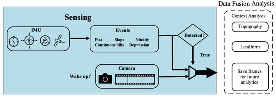
Figure 1.
Architecture of multiple-sensor-based sensing algorithm.
First, IMU sensors [18] are used as the main tool for data collection, especially in autonomous vehicle areas. Many existing solutions for motion tracking and gesture recognition rely on the IMU sensors’ built-in mobile devices [19]. Magnetic sensor [20,21] readings are used to determine device orientation changes, and in future may be applied to detect the detailed environment. Then, certain frames [22] can be captured with a trigger mechanism by the camera sensor mounted in the front of the robot for future analytics.
Next, analysis and data fusion are conducted on motion sensors’ data in real time with moving robot vehicles. The use of multiple sensors, such as a gyroscope [23] and an accelerometer [24], is advantageous because of the low-cost and easy combination, which makes it possible to collect continuous motion data in real time. With the data fusion algorithm, we can judge the topological information in real time according to the robot vehicle’s motion. If topological features change significantly, which we name it as an “event”, the camera is woken up to capture frames and saved them in association with the location on the map. This is for future reference of the current environment.
2. Related Work
2.1. Remote Monitoring
Agriculture industries traditionally implement optical and multispectral techniques on the images collected by satellites to analyze and evaluate the plant growth condition and yields [25]. The existence of chlorophyll, for instance, could be revealed by the light absorption from the leaf and, hence, determines plant health. It is of importance since decisions, such as fertilizing the soil and spreading insecticide or fungicide, should be taken based on this information. The treatments should be applied in time to ensure their functionality, requiring the filed information to be collected and analyzed frequently, which challenges the traditional method [26]. In addition, traditional monitoring methods are expensive to be implemented with regard to time efficiency. Remote sensing plays a critical role in precision agriculture by allowing farmers to collect various types of information to help improve the quality and yields of crops [27]. Optical remoting sensing, taking advantages of collected images by using visible and near infrared sensors to detect different target objects on the ground based on the radiation variation, has been utilized in many aspects of crop production [28]. Frolking et al. [29] developed new maps by combining the optical remote sensing and ground census data to investigate the diversity of rice production. Hall et al. [30] reviewed the applications of optical remoting sensing in viticulture by taking advantage of the information, such as soil structure and vine shape and size, from the collected images to ensure the quality and yields.
2.2. Motion Sensing
With the advancement of precise Global Positioning System (GPS) equipment and cameras detecting structures, various autonomous machines are employed in the agriculture sector [31]. The QUAD-AV project tested the performance of using microwave radar, stereo vision, LiDAR, and thermography to detect obstacles in the context of agriculture [32]. The project concluded that stereo vision stands out for its accuracy in ground and non-ground classification. Zhao et al. [33] proposed a method to gather road information on a large scale through the combination of phase cameras and motion sensors. An environment map was developed [34] for detecting the relative positions of nearby objects with multiple phone cameras. In addition, the turning movement of vehicles was captured by comparing the centrifugal force with a reference point. Then the authors extended this work by designing an efficient algorithm to reduce the computing time. Non-vision sensors are utilized in [35] to realize the detection of vehicle maneuvers, including lane changing, turning, and moving on a curvy path. Qi et al. [36] proposed to utilize the front- and rear-mounted cameras in a phone to identify dangerous road conditions. Chen et al. [37] developed a multiview 3D network to detect objects on the road, combined with a sensory-fusion framework to analyze data collected by LiDAR and cameras.
2.3. Robot Vehicles with Autonomoust Driving Techniques in Agriculture
Robots are gaining interest in precision agriculture due to the potential capability to automatically remove weeds and minimize the usage of pesticides and herbicides in crop production [38]. Different from the traditional methods that treat the whole field uniformly, robots apply resources to the target plants individually and, therefore, improve the resource efficiency. For this sake, the datasets focus on providing the field data to those who design automatic systems with robots to perform activities, such as classification, navigation, and mapping in modern agriculture [39].
2.4. Sensor Data Fusion in Agriculture
Fusion of sensor data has proved its capability in agriculture. Fusion of GPS and machine vision is leading the way to improve the applications of large machine guidance systems in agriculture. Plants cultivated in patterns facilitates the usage of autonomous machine systems with satisfying accuracy. However, the adverse environments where trees might disable the GPS signal negatively impact the system’s efficiency [40]. Acceleration data provided by the IMU devices compensate the impact of signal loss of GPS and ensure the accuracy of guidance systems. Therefore, the combination of GPS and IMU sensors can be implemented.
3. Methodology
3.1. IMU Sensor-Based Data Collection Approach
Two IMU sensors, a gyroscope, and an accelerometer were used to measure the attitude of an agricultural robot [41]. Inertial sensors come with intrinsic noises. To improve their usability and accuracy, we designed a coordinate alignment algorithm on both sloped surface and flat surface to detect sensor orientation changes and model stability. The proposed that the slope-aware algorithm first conduct coordinate alignment and estimate linear acceleration via dynamically withdrawing the gravity effect on recorded accelerometer readings. Then, it uses a clustering technique to identify relative orientation changes.
A gyroscope is an inertial sensor for measuring orientation based on the principles of angular momentum. However, because of noise jamming, temperature variation, and unstable force moment, algorithm drift error will occur and increase with time. Therefore, a gyroscope may have noise during a long period of data collection. A supplementary option is to use an accelerometer, which is a device that measures proper acceleration. When the accelerometer is motionless, the attitude angles can be calculated based on the acceleration of the gravity component in every axis via trigonometric functions.
Slope-Aware Alignment
The accuracy of coordinate alignment is mainly affected by the slope of the field. Hence, we developed a slope-aware coordinate alignment method to reduce or eliminate the negative effects caused by the slope. Traditional approaches fail to consider the slope, because they make the assumption that all the motion data is through the origin motion data point, and calculate the fit curve based on all motion data [42]. However, these approaches could encounter chaos with a random rough surface. Therefore, our slope-aware approach dynamically segments the whole path into pieces and uses each piece of the path as an independent input. Due to forces created by slopes, readings from each path deviate from the origin point. If we combine all the paths, we can estimate the slope and further improve the alignment accuracy. A rotation matrix will be derived by combining sensor readings from all paths. To derive the rotation matrix, we fitted the curve to find the direction unit vector. Different from traditional approaches, we trained the horizontal unit vector for each segment and combined them by assigning different weights for each segment. One segment will be selected if the recorded data indicates the car is in motion. The more data points we can include in this segment, the more we can increase the statistical power of the measurement.
As shown in Figure 2, the vector represents the orientation of a gyroscope sensor and represents the orientation of a robot vehicle. The rotation matrix can be estimated during the coordinate alignment process. In the rotation matrix , , , and are the unit coordinate conversion vectors along each demission, such that .
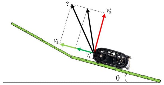
Figure 2.
Slope-aware rotation alignment concept.
3.2. Motion Pattern Recognition
Different field surfaces can lead to various accelerations and further affect the moving speed and motion patterns. Hence, recognizing motion patterns can help us understand the running environment of the robot vehicle. In this work, we use the dynamic time warping (DTW) algorithm to identify similar robot motions with varying speeds and further detecting running environments. The DTW algorithm is well known for evaluating the similarity between two temporal sequences. To measure the similarity, temporal sequences are “warped” by shrinking or stretching in the time domain. To achieve the best performance, the training set should be carefully prepared and include representatives of different types of events as much as possible. In order to improve detection accuracy, we chose to loosen some of the constraints of the DTW matching algorithms during the training process and also when conducting evaluations. As a theoretical result, our DTW algorithm was able to identify all the motions. There were four categories of motion patterns in our study as shown in Figure 3a–d.
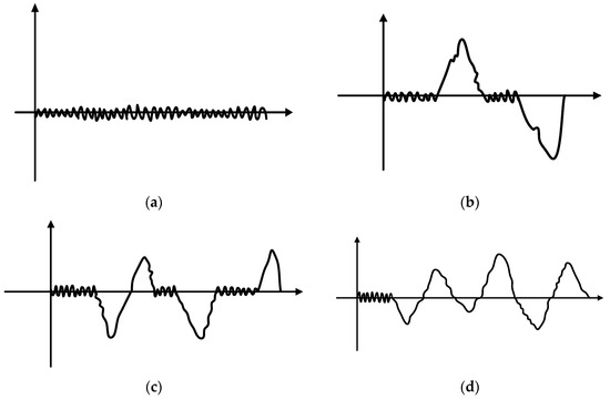
Figure 3.
Motion sensor theoretical patterns: (a) moving on a flat field; (b) moving over a slope; (c) moving across a depression; (d) moving on a muddy field.
3.3. Data Fusion Approach
The sensor fusion method avoids the measurement limitations of using only a camera. An advanced data fusion method was used to integrate data from the camera, accelerometer, and gyroscope [43]. In this study, two methods were discussed and compared. One is a self-adaptive complimentary principal component analysis (PCA) and the other one is the DTW.
Data collected from different sensors need to be synchronized as the clock on each device is different. After clock synchronization, we used principal component analysis (PCA) to speed up the data analysis process and detect various activities promptly as shown in Algorithm 1. PCA is able to extract the most important features from the collected dataset and convert a high-dimensional dataset to one with lower dimensions. PCA simplifies the dataset by discarding the least important features while maintaining the interpretability of variables.
| Algorithm 1. Pseudo-code of the algorithm for generating principal components |
| DTW (A, G) contains: |
| # A = (, …, ) is the accelerometer data. G = (, …, ) is the gyroscope data collected with continuous time series |
| -> Here, we claim M [0, … , n, 0, …, m] is a 2D data matrix which stands |
| for the similarity measures between the 2 timeseries. |
| # Data matrix initialization |
| -> M [0, 0]: = 0 |
| -> For i = 0 to m Step 1 Do: |
| -> M [0, i]: = Infinity |
| -> End |
| -> For i: = 1 to n Step 1 Do: |
| -> M [i, 0]: = Infinity |
| -> End |
| # Calculate the similarity measures between the 2 different time-series into M [n, m] |
| -> For i : = 1 to n Step 1 Do: |
| -> For j : = 1 to m Step 1 Do: |
| #Evaluate the similarity of the two points |
| -> diff : = |
| -> M [i, j] : = diff + Min (M [i-1, j], M [i, j-1], M [i-1, j-1]) |
| -> End |
| -> End |
| -> Return M [n, m] |
Additionally, PCA also combines original variables in such a way that only the most valuable features are retained. Hence, we extract features from our accelerometer and gyroscope dataset using the PCA algorithm. The algorithm is described by the following steps.
- Data Normalizationwhere is the mean and is the standard deviation of all the data.
- Covariance Matrix Calculationwhere represents the accelerometer readings and represents the gyroscope readings. Note that and .
is the covariance matrix, which is a matrix. The covariance matrix stores the covariance between two features. Once the covariance is established, PCA will perform the eigen decomposition on it. The covariance matrix can be calculated using the equations below:
where represents the mean vector, and it can be calculated using the following equation: The mean vector (d-dimensional vector) stores the mean of each feature column in the dataset.
- 3.
- Eigenvalue and Eigenvector Calculation
Next, we need to calculate the eigenvalues and eigenvectors for the covariance matrix. The covariance matrix is a square matrix, so the eigenvalue can be calculated using the characteristic equation below:
where, represents the eigenvalue for matrix , is an identity matrix which has the same dimension as to satisfy the requirement of matrix subtraction. “” is the determinant of the matrix. We can find a corresponding vector for each eigenvalue by solving the following equation:
- 4.
- Principal Component Selection
The eigenvalues are sorted in descending order such that they reflect the significance of the components. The eigenvector that has the highest eigenvalue is the principal component of the dataset. Given that our dataset contains two variables (accelerometer and gyroscope), we should have two eigenvalues and two eigenvectors. We use a feature vector to store the two eigenvectors.
- 5.
- Principle Component Formation
The eigenvectors represent the direction of the principal components. The original data need to be re-oriented to the new coordinate system using the eigenvectors. To re-orient the data, the original data were multiplied by the feature vector, and the re-oriented dataset is called a score as shown in Equation (7).
As discussed in previous sections, we built an event library (different motion patterns listed in Figure 3) using motion data collected by different robot vehicles. The motion data contain all the typical events. When a new event is detected, the corresponding motion data will be processed using the PCA algorithm and compared with all the predefined events in the event library. We used the DTW algorithm to evaluate the distance between the new event temporal sequence and all temporal sequences in the library. Based on the derived distance, a k-nearest neighbor algorithm was used to predict a label for the new event.
To evaluate the distance between two vectors, we used the following distance metrics. Euclidean distance—the root sum of squared differences:
Manhattan distance—the sum of absolute differences, also known as the Manhattan, city block, taxicab, or metric:
Squared distance—the square of the Euclidean metric:
Symmetric Kullback–Leibler metric distance—only valid when X and Y are real and positive numbers:
4. Experiment Design and System Implementation
4.1. System Design
A robot machine usually has limited battery capacities, so it is important to reduce unnecessary operations as much as possible if the machine is expected to do long-term work. Hence, it is better not to use the camera to monitor the machine during the whole trip, we only need to focus on some specific environmental images when an unusual topography is detected. Keeping this in mind, our algorithm leverages inertial sensors to continuously detect robot vehicle movement, only collecting corresponding camera data once an unusual motion pattern is detected. This, in addition to the fact that IMU sensors consume much less power than cameras, can dramatically decrease the energy requirement and the computing overhead of the whole algorithm.
4.2. System Implementation
Processing motion sensor data in real time is very important for our method. Additionally, capturing the associated environment images in time also offers accurate reference data for future analysis. Moreover, we also plan to add a real-time image processing function in future research. To achieve the best performance and extensibility, we chose an embedded computing platform and optimized the inference engine as the hardware container [44]. Our inference engine is optimized to run on this specific embedded computing platform [45,46]. In this work, we choose the NVIDIA Jetson TX2 embedded computer as the embedded computing platform. The Jetson TX2 has a hexcore ARMv8 64-bit CPU complex and a 256-core Pascal GPU. Our system is built upon the multithread framework, written in C and C++. We use independent pipelines to manage different tasks, e.g., we created a pipeline to collect data from motion sensors and monitor various events and implemented another pipeline to collect environment images. Each pipeline consists of a series of elements. The element is where a data stream is processed. In the hardware platform for small agricultural machine development, size and price are the two main parameters that must be considered in the design idea. In this study, we used a small-sized and low-cost IMU to capture acceleration and angular speed change.
4.3. Simulation Experiment Scenarios
In this study, we wanted to test our proposed algorithms and have precise control on knowing the terrain. Therefore, a simulation was built using a sand table that could easily create different terrain conditions. The sand table is a narrow rectangle that is like a downscaled racing track. During the data collection, we counted each run from one end of the sand table to the other end as one instance. To augment the datasets, we collected data with both ends as starting points and the other ends correspondingly as the end points. The different setups for each kind of terrain conditions as shown in Table 2 were chosen for the experimental tests. These simulated field conditions mainly included dry flat path, slope, depression, and muddy path. Each scenario was set up on the sand table. The lengths of these four experimental scenarios were approximately 2–3 m. Table 2 shows detailed information about each scenario. While the tested speeds of the robot vehicle in different scenarios vary according to the roughness of the fields, these speeds are helpful in guaranteeing high-quality data with proper passing period of each topography.
Table 2.
Indoor experiment scenarios.
4.4. Real-World Validation Experiment Scenarios
In this study, we collected the real-world field data with the vehicle (2019 Tacoma TRD Sport 4 × 4) as shown in Figure 4.
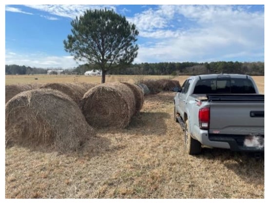
Figure 4.
The vehicle used for data collection.
Data collection activities included investigating and selecting locations of experiment scenarios in the field and collecting sensor data for various types of experiment scenarios. After the investigation in the field, four types of experiment scenarios were determined by researchers as shown in Table 3 with an IMU sensor. When collecting data for each experiment scenario, the researchers set the vehicle with a constant throttle to move straight forward with a fixed steering. The driving distance for each experiment scenario per trail was about 60 feet. Vehicle motion data in terms of gyroscope and acceleration (without g) were collected.
Table 3.
Real-world experiment scenarios.
5. Result and Discussion
We demonstrate and discuss the performance of our approach in recognizing dry flat surface field, slope, depression, and muddy field separately. In each scenario, a motion pattern and corresponding topological feature are plotted and discussed together in the following subsections. For different scenarios, we applied different speed and data collection rate setups for better quality data, and we also conducted some data processing, such as normalization, denoising, etc. Because the vehicle size and topological scale used for the simulated environment and the real-world field are significantly different, the ranges and slopes of both gyroscope and acceleration vary. However, our algorithm can still recognize the patterns with a data processing step.
5.1. Single Slope
As is shown in Figure 5, the field slopes were estimated using a gyroscope via coordinate alignment. The downslope with a sharply increasing incline and the downslope with a deep decrease are also marked. The derivative could easily address the gradient of the slope. If the gyroscope value drops down fast, then the slope is steep, while the slope has a minor gradient if the gyroscope value change is gradual. The results in Figure 5a give us an accordant pattern of slope detection in practice to the theoretical pattern. If, in some cases, the collected data could not perfectly match the pattern, the estimated linear acceleration was calculated as alignment using the accelerometer to reduce noise in the sensor data as shown in Figure 6. However, in most cases, the single slope could be recognized only using gyroscope data.
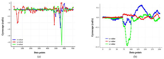
Figure 5.
Field slope with segmental gyroscope data: (a) simulated environment result; (b) real-world observed result.
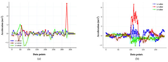
Figure 6.
Field slope with segmental linear acceleration data: (a) simulated result estimate; (b) real-world observed.
Figure 5b shows the real-world observed downslope from the field using a gyroscope via coordinate alignment. The climbing movement starts from around data point 100 and ends at around data point 175. The pattern is obvious and could be easily detected, but the noise from the observation, particularly at the end of the process, is significant. The results regarding the linear acceleration in Figure 6b, however, produce an unclear pattern of the downslope compared with the results from the gyroscope.
5.2. Depression or Soil Erosion
The depression can be identified from changes of values along the z-axis as shown in Figure 7. If the z-axis readings stay somewhat stable, then it should be a smooth field without bumps or depressions. If the readings start fluctuating, then there might exist a bump or depression. If the magnitude of readings along the z-axis changes from positive to negative, and readings of the x and the y axis also change, then it is very likely there is a depression. Similar patterns are also revealed by the real-world observed segmental gyroscope data collected from the experiments. The depression location starts from data point 100 and ends at around data point 270. The depressions between simulated environment and real-world environment are a little different in slope and distribution, so the valleys and peaks have different ranges. For example, the second valley in Figure 7a,b is different, but it was still recognized as similar to the second drop down according to pattern recognition.
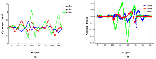
Figure 7.
Field depression with segmental gyroscope data: (a) simulated result estimate; (b) real-world observed.
5.3. Rough Field
The rough field is indicated by a continuous occurrence of bumps or depressions as shown in Figure 8a. If continuous peaks and valleys can be observed from z-axis values, then it is highly likely that there is a rough patch of the field. It can be divided into several depressions, which means the pattern of the rough field is a combination of depression patterns. The same pattern appears in the real-word observed segmental gyroscope data collected from the rough roads, shown in Figure 8b. With a short segment of the flat road before and after the rough segment, the fluctuations from all the directions continuously occur and show a clear pattern as estimated.
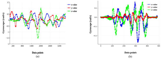
Figure 8.
Rough field with segmental gyroscope data: (a) simulated result estimate; (b) real-world observed.
5.4. Flat Field vs. Muddy Field
A muddy field could cause sudden deceleration as shown in Figure 9, where the muddy field starts from 9 s. The deceleration can be inferred from changes in readings along the y-axis. As we can see from this example, there is a deep valley at around 12 s, and the readings of both the x- and the z-axis are also fluctuating. Similar real-world results are shown in Figure 9b.

Figure 9.
Deceleration happens with the field surface changes: (a) Simulated result estimate; (b) real-world observed.
6. Conclusions and Future Work
Precision agriculture requires maps with localized topographies to properly adjust irrigation, route planning, and other crop management practices. Current approaches to this problem include the use of cameras and advanced computer vision algorithms or using distance sensors for gathering depth information for 3D map construction. Both methods are power-expensive, constraining their use. Our work presents an alternative method using a sensing algorithm with a low-cost, robot-vehicle-mounted, multidimensional map augmentation method that can track robot vehicle movements, monitor the surrounding environment by collecting key images, and link all the factors to the existing map, thereby providing useful analytics for task planning, route planning, and robot operators. The method leverages IMU sensors to gather mobility data for the robot vehicle. We also present data fusion techniques to detect topological changes in the field that could potentially cause a negative influence on farm machines. The results indicate this method works well and should lend itself to many useful agricultural applications.
In the future, we will continue exploring algorithms that can improve the robustness of this sensing method. Additionally, a deep neural network (DNN)–based mechanism will be developed that enables the algorithm to detect some categories of environmental objects alongside with the map points under good lighting conditions.
Author Contributions
Conceptualization, W.Z. and T.R.; methodology, W.Z.; software, W.Z.; validation, T.L., B.Q. and W.Z.; formal analysis, T.L.; investigation, Q.N.; resources, T.R.; data curation, Q.N.; writing—original draft preparation, W.Z.; writing—review and editing, T.R.; visualization, T.L.; supervision, T.R.; project administration, T.R.; funding acquisition, T.R. All authors have read and agreed to the published version of the manuscript.
Funding
This material is partially based upon work supported by the United States Department of Agriculture National Institute of Food and Agriculture, under ID number WIS02002.
Institutional Review Board Statement
Not applicable.
Informed Consent Statement
Not applicable.
Data Availability Statement
Data available on request due to restrictions eg privacy or ethical.
Conflicts of Interest
The authors declare no conflict of interest.
References
- Badgley, C.; Moghtader, J.; Quintero, E.; Zakem, E.; Chappell, M.J.; Aviles-Vazquez, K.; Perfecto, I. Organic agriculture and the global food supply. Renew. Agric. Food Syst. 2007, 22, 86–108. [Google Scholar] [CrossRef]
- Rosenzweig, C.; Parry, M.L. Potential impact of climate change on world food supply. Nature 1994, 367, 133–138. [Google Scholar] [CrossRef]
- Hussnain, M.; Sharjeel, M.; Chaudhry, S.R.; Hussain, S.A.; Raza, I.; Mirza, J.S. Investigating multi-topological zigbee based wireless sensor network in precision agriculture. J. Basics Appl. Sci. Res. 2013, 3, 195–201. [Google Scholar]
- Mareels, I.; Weyer, E.; Ooi, S.K.; Cantoni, M.; Li, Y.; Nair, G. Systems engineering for irrigation systems: Successes and challenges. IFAC Proc. Vol. 2005, 38, 1–16. [Google Scholar] [CrossRef]
- Myalo, O.V.; Myalo, V.V.; Prokopov, S.P.; Solomkin, A.P.; Soynov, A.S. Theoretical substantiation of machine-tractor fleet technical maintenance system on the example of Omsk region agricultural enterprises. Ser. J. Phys. Conf. Ser. 2018, 1059, 012005. [Google Scholar] [CrossRef]
- Nandurkar, S.R.; Thool, V.R.; Thool, R.C. Design and development of precision agriculture system using wireless sensor network. In Proceedings of the 2014 First International Conference on Automation, Control, Energy and Systems (ACES), Adisaptagram, India, 1–2 February 2014; Neumeier, S., Wintersberger, P., Frison, A.K., Becher, A., Facchi, C., Riener, A., Eds.; IEEE: New York, NY, USA, 2014. [Google Scholar]
- Prakash, A. Thermal remote sensing: Concepts, issues and applications. Int. Arch. Photogramm. Remote Sens. 2000, 33, 239–243. [Google Scholar]
- Shafian, S.; Maas, S.J. Index of soil moisture using raw Landsat image digital count data in Texas high plains. Remote Sens. 2015, 7, 2352–2372. [Google Scholar] [CrossRef]
- Gonzalez-Dugo, V.; Zarco-Tejada, P.; Berni, J.A.; Suárez, L.; Goldhamer, D.; Fereres, E. Almond tree canopy temperature reveals intra-crown variability that is water stress-dependent. Agric. For. Meteorol. 2012, 154, 156–165. [Google Scholar] [CrossRef]
- Berdugo, C.A.; Zito, R.; Paulus, S.; Mahlein, A.K. Fusion of sensor data for the detection and differentiation of plant diseases in cucumber. Plant Pathol. 2014, 63, 1344–1356. [Google Scholar] [CrossRef]
- Honkavaara, E.; Saari, H.; Kaivosoja, J.; Pölönen, I.; Hakala, T.; Litkey, P.; Pesonen, L. Processing and assessment of spectrometric, stereoscopic imagery collected using a lightweight UAV spectral camera for precision agriculture. Remote Sens. 2013, 5, 5006–5039. [Google Scholar] [CrossRef]
- Costa, F.G.; Ueyama, J.; Braun, T.; Pessin, G.; Osório, F.S.; Vargas, P.A. The use of unmanned aerial vehicles and wireless sensor network in agricultural applications. In Proceedings of the 2012 IEEE International Geoscience and Remote Sensing Symposium, Munich, Germany, 22–27 July 2012; IEEE: New York, NY, USA, 2012. [Google Scholar]
- Maes, W.H.; Steppe, K. Perspectives for remote sensing with unmanned aerial vehicles in precision agriculture. Trends Plant Sci. 2019, 24, 152–164. [Google Scholar] [CrossRef]
- Matsuzaki, S.; Masuzawa, H.; Miura, J.; Oishi, S. 3D Semantic Mapping in Greenhouses for Agricultural Mobile Robots with Robust Object Recognition Using Robots’ Trajectory. In Proceedings of the 2018 IEEE International Conference on Systems, Man, and Cybernetics (SMC), Miyazaki, Japan, 7–10 October 2018; IEEE: New York, NY, USA, 2018. [Google Scholar]
- Nadkarni, P.M. Management of evolving map data: Data structures and algorithms based on the framework map. Genomics 1995, 30, 565. [Google Scholar] [CrossRef]
- Li, L.; Yao, J.; Xie, R.; Tu, J.; Chen, F. Laser-Based Slam with Efficient Occupancy Likelihood Map Learning for Dynamic Indoor Scenes. ISPRS Ann. Photogramm. Remote Sens. Spat. Inf. 2016, 3, 119–126. [Google Scholar] [CrossRef]
- Chen, F.; Wang, J.M.; Sun, B.G.; Chen, X.M.; Yang, Z.X.; Duan, Z.Y. Relationships of plant species distribution in different strata of Pinus yunnanensis forest with landform and climatic factors. Chin. J. Ecol. 2012, 31, 1070. [Google Scholar]
- Won, S.H.P.; Golnaraghi, F.; Melek, W.W. A Fastening Tool Tracking System Using an IMU and a Position Sensor With Kalman Filters and a Fuzzy Expert System. IEEE Trans. Ind. Electron. 2009, 56, 1782–1792. [Google Scholar] [CrossRef]
- Feng, T.; Liu, Z.; Kwon, K.A.; Shi, W.; Carbunar, B.; Jiang, Y.; Nguyen, N. Continuous mobile authentication using touchscreen gestures. In Proceedings of the 2012 IEEE Conference On Technologies For Homeland Security (HST), Waltham, MA, USA, 13–15 November 2012; IEEE: New York, NY, USA, 2012. [Google Scholar]
- Hu, C.; Li, M.; Song, S.; Zhang, R.; Meng, M.Q.H. A Cubic 3-Axis Magnetic Sensor Array for Wirelessly Tracking Magnet Position and Orientation. IEEE Sens. J. 2010, 10, 903–913. [Google Scholar] [CrossRef]
- Zhao, W.; Xu, L.; Bai, J.; Ji, M.; Runge, T. Sensor-based risk perception ability network design for drivers in snow and ice environmental freeway: A deep learning and rough sets approach. Soft Comput. 2018, 22, 1457–1466. [Google Scholar] [CrossRef]
- Zhao, W.; Yamada, W.; Li, T.; Digman, M.; Runge, T. Augmenting Crop Detection for Precision Agriculture with Deep Visual Transfer Learning—A Case Study of Bale Detection. Remote Sens. 2021, 13, 23. [Google Scholar] [CrossRef]
- Mayagoitia, R.E.; Nene, A.V.; Veltink, P.H. Accelerometer and rate gyroscope measurement of kinematics: An inexpensive alternative to optical motion analysis systems. J. Biomech. 2002, 35, 537–542. [Google Scholar] [CrossRef]
- Bouten, C.V.; Koekkoek, K.T.; Verduin, M.; Kodde, R.; Janssen, J.D. A triaxial accelerometer and portable data processing unit for the assessment of daily physical activity. IEEE Trans. Biomed. Eng. 1997, 44, 136–147. [Google Scholar] [CrossRef] [PubMed]
- Mulla, D.J. Twenty five years of remote sensing in precision agriculture: Key advances and remaining knowledge gaps. Biosyst. Eng. 2013, 114, 358–371. [Google Scholar] [CrossRef]
- Zhang, C.; Kovacs, J.M. The application of small unmanned aerial systems for precision agriculture: A review. Precis. Agric. 2012, 13, 693–712. [Google Scholar] [CrossRef]
- Mahlein, A.K. Plant disease detection by imaging sensors–parallels and specific demands for precision agriculture and plant phenotyping. Plant Dis. 2016, 100, 241–251. [Google Scholar] [CrossRef] [PubMed]
- Neumeier, S.; Wintersberger, P.; Frison, A.K.; Becher, A.; Facchi, C.; Riener, A. Teleoperation: The holy grail to solve problems of automated driving? Sure, but latency matters. In Proceedings of the 11th International Conference on Automotive User Interfaces and Interactive Vehicular Applications, Utrecht, The Netherlands, 21–25 September 2019; pp. 186–197. [Google Scholar]
- Frolking, S.; Qiu, J.; Boles, S.; Xiao, X.; Liu, J.; Zhuang, Y.; Qin, X. Combining remote sensing and ground census data to develop new maps of the distribution of rice agriculture in China. Glob. Biogeochem. Cycles 2002, 16, 38-1–38-10. [Google Scholar] [CrossRef]
- Hall, A.; Lamb, D.W.; Holzapfel, B.; Louis, J. Optical remote sensing applications in viticulture—A review. Aust. J. Grape Wine Res. 2002, 8, 36–47. [Google Scholar] [CrossRef]
- Anderson, N.W. Method and System for Identifying an Edge of a Plant. U.S. Patent 7,916,898, 29 March 2011. [Google Scholar]
- Rouveure, R.; Nielsen, M.; Petersen, A.; Reina, G.; Foglia, M.; Worst, R.; Seyed-Sadri, S.; Blas, M.R.; Faure, P.; Milella, A.; et al. The QUAD-AV Project: Multi-sensory approach for obstacle detection in agricultural autonomous robotics. In Proceedings of the 2012 International Conference of Agricultural Engineering CIGR-Ageng, Valencia, Spain, 8–12 July 2012. [Google Scholar]
- Zhao, W.; Yin, J.; Wang, X.; Hu, J.; Qi, B.; Runge, T. Real-time vehicle motion detection and motion altering for connected vehicle: Algorithm design and practical applications. Sensors 2019, 19, 4108. [Google Scholar] [CrossRef] [PubMed]
- Beall, C.; Dellaert, F. Appearance-based localization across seasons in a metric map. In Proceedings of the IROS Workshop on Planning, Perception and Navigation for Intelligent Vehicles (PPNIV), Chicago, IL, USA, 16 September 2014. [Google Scholar]
- Estes, R.A.; Bynum, J.R.; Riggs, R. Gyroscopic Steering Tool Using Only a Two-Axis Rate Gyroscope and Deriving the Missing Third Axis. U.S. Patent 7,234,540, 26 June 2007. [Google Scholar]
- Qi, B.; Liu, P.; Ji, T.; Zhao, W.; Banerjee, S. DrivAid: Augmenting driving analytics with multi-modal information. In Proceedings of the 2018 IEEE Vehicular Networking Conference (VNC), Taipei, Taiwan, 5–7 December 2018; IEEE: New York, NY, USA, 2018; pp. 1–8. [Google Scholar]
- Chen, X.; Ma, H.; Wan, J.; Li, B.; Xia, T. Multi-view 3d object detection network for autonomous driving. In Proceedings of the IEEE Conference on Computer Vision and Pattern Recognition, Honolulu, HI, USA, 21–26 July 2017; pp. 1907–1915. [Google Scholar]
- Pretto, A.; Aravecchia, S.; Burgard, W.; Chebrolu, N.; Dornhege, C.; Falck, T.; Liebisch, F. Building an Aerial-Ground Robotics System for Precision Farming. arXiv 2019, arXiv:1911.03098. [Google Scholar]
- Lepej, P.; Rakun, J. Simultaneous localisation and mapping in a complex field environment. Biosyst. Eng. 2016, 150, 160–169. [Google Scholar] [CrossRef]
- Abbasi, A.Z.; Islam, N.; Shaikh, Z.A. A review of wireless sensors and networks’ applications in agriculture. Comput. Stand. Interfaces 2014, 36, 263–270. [Google Scholar]
- Zhao, W.; Wang, W.; Wang, X.; Jin, Z.; Li, Y.; Runge, T. A low-cost simultaneous localization and mapping algorithm for last-mile delivery. In Proceedings of the 2019 5th International Conference on Transportation Information and Safety (ICTIS), Liverpool, UK, 14–17 July 2019. [Google Scholar]
- Kang, L.; Zhao, W.; Qi, B.; Banerjee, S. Augmenting self-driving with remote control: Challenges and directions. In Proceedings of the 19th International Workshop on Mobile Computing Systems & Applications, New York, NY, USA, 14–18 February 2018; pp. 19–24. [Google Scholar]
- Li, T.; Kockelman, K.M. Valuing the safety benefits of connected and automated vehicle technologies. In Proceedings of the Transportation Research Board 95th Annual Meeting, Washington, DC, USA, 10–14 January 2016; Volume 1. [Google Scholar]
- Wang, X.; An, K.; Tang, L.; Chen, X. Short term prediction of freeway exiting volume based on SVM and KNN. Int. J. Transp. Sci. Technol. 2015, 4, 337–352. [Google Scholar] [CrossRef]
- Zhao, W.; Xu, L.; Qi, B.; Hu, J.; Wang, T.; Runge, T. Vivid: Augmenting vision-based indoor navigation system with edge computing. IEEE Access 2020, 8, 42909–42923. [Google Scholar] [CrossRef]
- Zhao, W.; Wang, X.; Qi, B.; Runge, T. Ground-level Mapping and Navigating for Agriculture based on IoT and Computer Vision. IEEE Access 2020, 8, 221975–221985. [Google Scholar] [CrossRef]
Publisher’s Note: MDPI stays neutral with regard to jurisdictional claims in published maps and institutional affiliations. |
© 2021 by the authors. Licensee MDPI, Basel, Switzerland. This article is an open access article distributed under the terms and conditions of the Creative Commons Attribution (CC BY) license (http://creativecommons.org/licenses/by/4.0/).