
Investigating Sustainable Commuting Patterns by Socio-Economic Factors


Abstract
1. Introduction
2. Literature Review
3. Methodologies
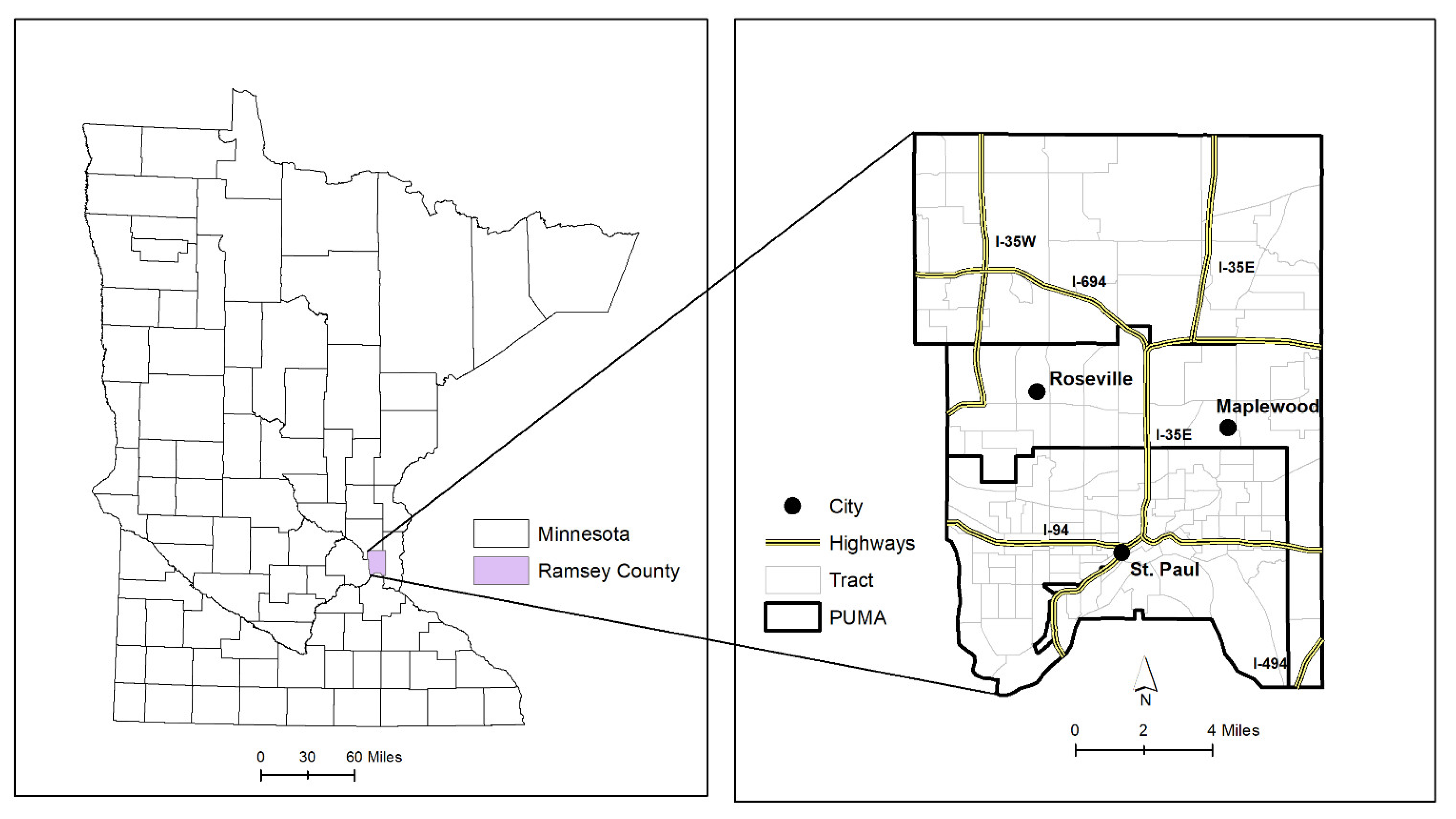
3.1. Study Area
3.2. Data
3.3. Method
4. Results
5. Discussion
6. Conclusions and Future Outlooks
Author Contributions
Funding
Institutional Review Board Statement
Informed Consent Statement
Data Availability Statement
Conflicts of Interest
References
- Antipova, A.A. Analysis of Commuting Distances of Low-Income Workers in Memphis Metropolitan Area, TN. Sustainability 2020, 12, 1209. [Google Scholar] [CrossRef]
- Kim, C.; Sang, S.; Chun, Y.; Lee, W. Exploring urban commuting imbalance by jobs and gender. Appl. Geogr. 2012, 32, 532–545. [Google Scholar] [CrossRef]
- Jang, W.; Yao, X. Tracking Ethnically Divided Commuting Patterns Over Time: A Case Study of Atlanta. Prof. Geogr. 2014, 66, 274–283. [Google Scholar] [CrossRef]
- Heath, Y.; Gifford, R. Extending the Theory of Planned Behavior: Predicting the Use of Public Transportation1. J. Appl. Soc. Psychol. 2002, 32, 2154–2189. [Google Scholar] [CrossRef]
- Boto-Álvarez, A.; García-Fernández, R. Implementation of the 2030 Agenda Sustainable Development Goals in Spain. Sustainability 2020, 12, 2546. [Google Scholar] [CrossRef]
- D’Adamo, I.; Rosa, P. How Do You See Infrastructure? Green Energy to Provide Economic Growth after COVID-19. Sustainability 2020, 12, 4738. [Google Scholar] [CrossRef]
- Molina, J.A.; Giménez-Nadal, J.I.; Velilla, J. Sustainable Commuting: Results from a Social Approach and International Evidence on Carpooling. Sustainability 2020, 12, 9587. [Google Scholar] [CrossRef]
- Bergman, Z.; Bergman, M.M. A Case Study of the Sustainable Mobility Problem–Solution Paradox: Motility and Access of Metrorail Commuters in the Western Cape. Sustainability 2019, 11, 2842. [Google Scholar] [CrossRef]
- American Public Transport Association. Who Rides Public Transportation. 2017. Available online: https://community-wealth.org/sites/clone.community-wealth.org/files/downloads/who%20rides%20public%20transportation.pdf (accessed on 5 January 2021).
- Shaw, C.B.; Gallent, N. Sustainable Commuting: A Contradiction In Terms? Reg. Stud. 1999, 33, 274–280. [Google Scholar] [CrossRef]
- Gojanovic, B.; Welker, J.; Iglesias, K.; Daucourt, C.; Gremion, G. Electric Bicycles as a New Active Transportation Modality to Promote Health. Med. Sci. Sports Exerc. 2011, 43, 2204–2210. [Google Scholar] [CrossRef] [PubMed]
- Koglin, T.; Rye, T. The marginalisation of bicycling in Modernist urban transport planning. J. Transp. Heal. 2014, 1, 214–222. [Google Scholar] [CrossRef]
- Thuany, M.; Melo, J.C.N.; Tavares, J.P.B.; Santos, F.M.J.; Silva, E.C.M.; Werneck, A.O.; Dantas, S.; Ferrari, G.; Sá, T.H.; Silva, D.R. The Profile of Bicycle Users, Their Perceived Difficulty to Cycle, and the Most Frequent Trip Origins and Destinations in Aracaju, Brazil. Int. J. Environ. Res. Public Health 2020, 17, 7983. [Google Scholar] [CrossRef]
- Moslem, S.; Campisi, T.; Szmelter-Jarosz, A.; Duleba, S.; Nahiduzzaman, K.M.; Tesoriere, G. Best–Worst Method for Modelling Mobility Choice after COVID-19: Evidence from Italy. Sustainability 2020, 12, 6824. [Google Scholar] [CrossRef]
- Ajzen, I. The theory of planned behavior. Organ. Behav. Hum. Decis. Process. 1991, 50, 179–211. [Google Scholar] [CrossRef]
- Peng, J.; Juan, Z.-C. The Theory of Planned Behavior: The Role of Descriptive Norms and Habit in the Prediction of Intercity Travel Mode Choice. J. Converg. Inf. Technol. 2013, 8, 211–219. [Google Scholar]
- Lois, D.; Moriano, J.A.; Rondinella, G. Cycle commuting intention: A model based on theory of planned behaviour and social identity. Transp. Res. Part F Traffic Psychol. Behav. 2015, 32, 101–113. [Google Scholar] [CrossRef]
- Chen, K.; Liang, H. Factors Affecting Consumers’ Green Commuting. Eurasia J. Math. Sci. Technol. Educ. 2016, 12, 527–538. [Google Scholar] [CrossRef]
- Chen, K.; Liang, H.; Wang, X. Psychological Divergence Between Urban and Suburban Chinese in Relation to Green Commuting. Soc. Behav. Pers. Int. J. 2016, 44, 481–498. [Google Scholar] [CrossRef]
- Song, Y.; Shao, G.; Song, X.; Liu, Y.; Pan, L.; Ye, H. The Relationships between Urban Form and Urban Commuting: An Empirical Study in China. Sustainability 2017, 9, 1150. [Google Scholar] [CrossRef]
- Gao, K.; Shao, M.; Sun, L. Roles of Psychological Resistance to Change Factors and Heterogeneity in Car Stickiness and Transit Loyalty in Mode Shift Behavior: A Hybrid Choice Approach. Sustainability 2019, 11, 4813. [Google Scholar] [CrossRef]
- Liu, C.; Cao, M.; Yang, T.; Ma, L.; Wu, M.; Cheng, L.; Ye, R. Inequalities in the commuting burden: Institutional constraints and job-housing relationships in Tianjin, China. Res. Transp. Bus. Manag. 2020, 100545. [Google Scholar] [CrossRef]
- Fan, J.X.; Wen, M.; Kowaleski-Jones, L. An ecological analysis of environmental correlates of active commuting in urban U.S. Health Place 2014, 30, 242–250. [Google Scholar] [CrossRef]
- Kim, C.; Choi, C. Towards Sustainable Urban Spatial Structure: Does Decentralization Reduce Commuting Times? Sustainability 2019, 11, 1012. [Google Scholar] [CrossRef]
- Oviedo, D.; Guzman, L.A. Revisiting Accessibility in a Context of Sustainable Transport: Capabilities and Inequalities in Bogotá. Sustainability 2020, 12, 4464. [Google Scholar] [CrossRef]
- Levin, L. How May Public Transport Influence the Practice of Everyday Life among Younger and Older People and How May Their Practices Influence Public Transport? Soc. Sci. 2019, 8, 96. [Google Scholar] [CrossRef]
- Delbosc, A.; Currie, G. The spatial context of transport disadvantage, social exclusion and well-being. J. Transp. Geogr. 2011, 19, 1130–1137. [Google Scholar] [CrossRef]
- Zhao, F.; Park, N. Using Geographically Weighted Regression Models to Estimate Annual Average Daily Traffic. Transp. Res. Rec. J. Transp. Res. Board 2004, 1879, 99–107. [Google Scholar] [CrossRef]
- Chiou, Y.-C.; Jou, R.-C.; Yang, C.-H. Factors affecting public transportation usage rate: Geographically weighted regression. Transp. Res. Part A Policy Pr. 2015, 78, 161–177. [Google Scholar] [CrossRef]
- Bai, T.; Li, X.; Sun, Z. Effects of cost adjustment on travel mode choice: Analysis and comparison of different logit models. Transp. Res. Procedia 2017, 25, 2649–2659. [Google Scholar] [CrossRef]
- Hasnine, M.S.; Lin, T.; Weiss, A.; Habib, K.N. Determinants of travel mode choices of post-secondary students in a large metropolitan area: The case of the city of Toronto. J. Transp. Geogr. 2018, 70, 161–171. [Google Scholar] [CrossRef]
- Liu, X.; Gao, L.; Ni, A.; Ye, N. Understanding Better the Influential Factors of Commuters’ Multi-Day Travel Behavior: Evidence from Shanghai, China. Sustainability 2020, 12, 376. [Google Scholar] [CrossRef]
- Ding, L.; Zhang, N. A Travel Mode Choice Model Using Individual Grouping Based on Cluster Analysis. Procedia Eng. 2016, 137, 786–795. [Google Scholar] [CrossRef]
- Cheng, L.; Chen, X.; De Vos, J.; Lai, X.; Witlox, F. Applying a random forest method approach to model travel mode choice behavior. Travel Behav. Soc. 2019, 14, 1–10. [Google Scholar] [CrossRef]
- Jing, P.; Zhao, M.; He, M.; Chen, L. Travel Mode and Travel Route Choice Behavior Based on Random Regret Minimization: A Systematic Review. Sustainability 2018, 10, 1185. [Google Scholar] [CrossRef]
- Ganciu, A.; Balestrieri, M.; Imbroglini, C.; Toppetti, F. Dynamics of Metropolitan Landscapes and Daily Mobility Flows in the Italian Context. An Analysis Based on the Theory of Graphs. Sustainability 2018, 10, 596. [Google Scholar] [CrossRef]
- Rademacher, N. How and where Minnesota’s population grew in the last decade, StarTribune. 12 April 2020. Available online: https://www.startribune.com/how-and-where-minnesota-s-population-grew-in-the-last-decade/569315761/ (accessed on 7 December 2020).
- Minnesota Compass, Ramsey County data. Available online: https://www.mncompass.org/profiles/county/ramsey (accessed on 5 November 2020).
- Ramsey County. 2040 Land Use Forecasts and Community Designation, Ramsey County Comprehensive Plan. Available online: https://www.ramseycounty.us/sites/default/files/Departments/Policy%20and%20Planning/RamseyCounty2040_Land%20Use.pdf (accessed on 13 December 2020).
- Yuan, F.; Sawaya, K.E.; Loeffelholz, B.C.; Bauer, M.E. Land cover classification and change analysis of the Twin Cities (Minnesota) Metropolitan Area by multitemporal Landsat remote sensing. Remote Sens. Environ. 2005, 98, 317–328. [Google Scholar] [CrossRef]
- Minnesota Department of Transportation (MNDOT). Ramsey County Highway Map. Available online: https://web.archive.org/web/20171230221457/http:/www.dot.state.mn.us/maps/gdma/data/maps/county/ramsey.pdf (accessed on 7 December 2020).
- Ramsey County Public Works Department (RCPWD). Ramsey County Public Works Department 2017–2021 Transportation Improvement Plan. Available online: https://web.archive.org/web/20171230214627/https:/www.ramseycounty.us/sites/default/files/Roads%20and%20Transit/2017-2021%20Transportation%20Improvement%20Program.pdf (accessed on 7 December 2020).
- American Association of State Highway and Transportation (AASHTO). Available online: https://ctpp.transportation.org/ (accessed on 1 September 2020).
- Brunsdon, C.; Fotheringham, A.S.; Charlton, M.E. Geographically Weighted Regression: A Method for Exploring Spatial Nonstationarity. Geogr. Anal. 1996, 28, 281–298. [Google Scholar] [CrossRef]
- Horner, M.W.; Murray, A.T. Excess Commuting and the Modifiable Areal Unit Problem. Urban Stud. 2002, 39, 131–139. [Google Scholar] [CrossRef]
- Sultana, S. Job/Housing Imbalance and Commuting Time in the Atlanta Metropolitan Area: Exploration of Causes of Longer Commuting Time. Urban Geogr. 2002, 23, 728–749. [Google Scholar] [CrossRef]
- O’Kelly, M.E.; Lee, W. Disaggregate Journey-to-Work Data: Implications for Excess Commuting and Jobs–Housing Balance. Environ. Plan. A Econ. Space 2005, 37, 2233–2252. [Google Scholar] [CrossRef]
- United States Census Bureau, Poverty Thresholds. 2016. Available online: https://www.census.gov/data/tables/time-series/demo/income-poverty/historical-poverty-thresholds.html (accessed on 5 September 2020).
- Yap, B.W.; Sim, C.H. Comparisons of various types of normality tests. J. Stat. Comput. Simul. 2011, 81, 2141–2155. [Google Scholar] [CrossRef]
- ACS Commuter Data Visualizations. 2016. Available online: http://ilikebigbytes.com/index.php/2016/05/18/acs-commuter-data-visualizations/ (accessed on 30 December 2020).
- Bureau of Transportation Statistics. National Transportation Statistics 2/27/2020 Updates, Principal Means of Transportation to Work and other categories. Available online: https://www.bts.dot.gov/newsroom/national-transportation-statistics-02272020 (accessed on 10 October 2020).
- Serulle, N.U.; Cirillo, C. Transportation needs of low income population: A policy analysis for the Washington D.C. metropolitan region. Public Transp. 2016, 8, 103–123. [Google Scholar] [CrossRef]


| Variable | Min. | Max. | Sum | Mean | Std. Dev. |
|---|---|---|---|---|---|
| Sustainable commuting | 8 | 7165 | 48,918 | 357.07 | 712.23 |
| Drive alone | 25 | 17,940 | 229,355 | 1674.12 | 2523.82 |
| Poverty | 0 | 1050 | 15,885 | 115.95 | 146.24 |
| Minority group | 0 | 4065 | 61,410 | 448.25 | 586.35 |
| Older worker (65 and above) | 0 | 870 | 12,401 | 90.52 | 121.18 |
| Kolmogorov–Smirnov | Shapiro–Wilk | |||
|---|---|---|---|---|
| Variable | Statistic | Sig. | Statistic | Sig. |
| Sustainable Commuting | 0.312 | 0.000 *** | 0.388 | 0.000 *** |
| Drive alone | 0.268 | 0.000 *** | 0.578 | 0.000 *** |
| LnSC | 0.066 | 0.200 | 0.985 | 0.126 |
| LnCar | 0.049 | 0.200 | 0.993 | 0.790 |
| Model | Variable | Coefficient | T-Statistic | p-Value |
|---|---|---|---|---|
| 1. Sustainable commuting | Constant | 1.9598 | 56.9315 | 0.0000 *** |
| ( 0.5832) | Poverty | 0.0007 | 1.9140 | 0.0578 * |
| Minority group | 0.0003 | 2.8703 | 0.0048 *** | |
| Older worker (65+) | 0.0005 | 1.1330 | 0.2592 | |
| 2. Drive alone | Constant | 2.6352 | 70.3983 | 0.000 *** |
| ( 0.5616) | Poverty | 0.0004 | −1.1473 | 0.2533 |
| Minority group | 0.0001 | 3.8804 | 0.0001 *** | |
| Older worker (65+) | 0.0012 | 2.1324 | 0.0348 ** |
| Model | OLS | GWR | ||
|---|---|---|---|---|
| AIC | AIC | |||
| 1. Sustainable Commuting | 0.5832 | 76.3980 | 0.6676 | 69.3223 |
| 2. Drive alone | 0.5616 | 99.3592 | 0.6771 | 81.3361 |
| PUMA | 1301 North) | 1302 (Central) | 1303 (Southeast) | 1304 (Southwest) | |
|---|---|---|---|---|---|
| 1301 | 120 (2.8%) | 46 (1.0%) | 31 (0.7%) | 45 (1.0%) | 243 (5.6%) |
| 1302 | 230 (5.3%) | 232 (5.3%) | 181 (4.2%) | 235 (5.4%) | 878 (20.1%) |
| 1303 | 222 (5.1%) | 206 (4.7%) | 587 (13.5%) | 412 (9.5%) | 1427 (32.7%) |
| 1304 | 228 (5.2%) | 271 (6.2%) | 368 (8.4%) | 944 (21.6%) | 1812 (41.6%) |
| 800 (18.4%) | 754 (17.3%) | 1168 (26.8%) | 1636 (37.5%) | 4359 (100.0%) |
| PUMA | 1301 (North) | 1302 (Central) | 1303 (Southeast) | 1304 (Southwest) | |
|---|---|---|---|---|---|
| 1301 | 536 (12.9%) | 75 (1.8%) | 32 (0.8%) | 35 (0.8%) | 679 (16.3%) |
| 1302 | 332 (8.0%) | 283 (6.8%) | 105 (2.5%) | 87 (2.1%) | 807 (19.4%) |
| 1303 | 312 (7.5%) | 195 (4.7%) | 602 (14.5%) | 222 (5.3%) | 1331 (32.0%) |
| 1304 | 280 (6.7%) | 161 (3.9%) | 259 (6.2%) | 642 (15.4%) | 1343 (32.3%) |
| 1461 (35.1%) | 715 (17.2%) | 998 (24.0%) | 985 (23.7%) | 4160 (100.0%) |
Publisher’s Note: MDPI stays neutral with regard to jurisdictional claims in published maps and institutional affiliations. |
© 2021 by the authors. Licensee MDPI, Basel, Switzerland. This article is an open access article distributed under the terms and conditions of the Creative Commons Attribution (CC BY) license (http://creativecommons.org/licenses/by/4.0/).
Share and Cite
Jang, W.; Yuan, F.; Lopez, J.J. Investigating Sustainable Commuting Patterns by Socio-Economic Factors. Sustainability 2021, 13, 2180. https://doi.org/10.3390/su13042180
Jang W, Yuan F, Lopez JJ. Investigating Sustainable Commuting Patterns by Socio-Economic Factors. Sustainability. 2021; 13(4):2180. https://doi.org/10.3390/su13042180
Chicago/Turabian StyleJang, Woo, Fei Yuan, and Jose Javier Lopez. 2021. "Investigating Sustainable Commuting Patterns by Socio-Economic Factors" Sustainability 13, no. 4: 2180. https://doi.org/10.3390/su13042180
APA StyleJang, W., Yuan, F., & Lopez, J. J. (2021). Investigating Sustainable Commuting Patterns by Socio-Economic Factors. Sustainability, 13(4), 2180. https://doi.org/10.3390/su13042180