GIS-Enabled Digital Twin System for Sustainable Evaluation of Carbon Emissions: A Case Study of Jeonju City, South Korea

Abstract
1. Introduction
1.1. Background
- (1)
- How can DT technologies or ideas reduce carbon emissions?
- (2)
- How can DTs assist in improving current decision-making processes to lessen failures of new planning?
- (3)
- What are the roles of DTs in geospatial analyses or technology fields?
- (4)
- What types of Fourth Industrial Revolution technologies can be combined with the new DTs?
- First, this study contributes to the current definitions of DTs in geospatial technology. As stated earlier, the DT has been booming in the manufacturing field, but its definition in geospatial technology has not been clearly defined yet.
- Second, this study also guides what technologies are associated with the DT environment or system. Even though a DT system can computerize counterparts of a physical world, it is not merely a digital component of a physical world. Employment of a DT system is not just construction of 3D city models. Thus, it is necessary for city planners or geospatial analysts to comprehend how to establish new skills, particularly connected with the Internet of Things (IoT) technologies. This can help us clearly comprehend how DTs contribute to the digital transformation of society.
- Third, the construction of DTs can help urban areas to become more environmentally and economically sustainable because the DT environment enables urban planners to simulate urban planning models that help cities face complex issues such as disasters, carbon emission or infectious diseases like the coronavirus pandemic.
- In addition, through this research we expect that the DTs in geospatial technology will bring up a variety of benefits such as efficiency of services, sustainability, safety, economic growth, and more for smart cities.
- As such, the DTs in geospatial technology can experimentally mirror real-world problems and resolve urban environmental issues such as carbon emission. Accordingly, this study will help communicate with the general public wanting to acquire carbon emissions information on a local scale.
1.2. Previous Studies
- (1)
- What are the optimal geospatial technologies to employ GIS-enabled DT systems for carbon emissions?
- (2)
- What if we develop scenario-based approaches to mitigate the risk of carbon emissions? What would happen if we change this?
- (3)
- How can an urban planner deliver carbon-related information to citizens in real-time?
2. Materials and Methods
2.1. Materials
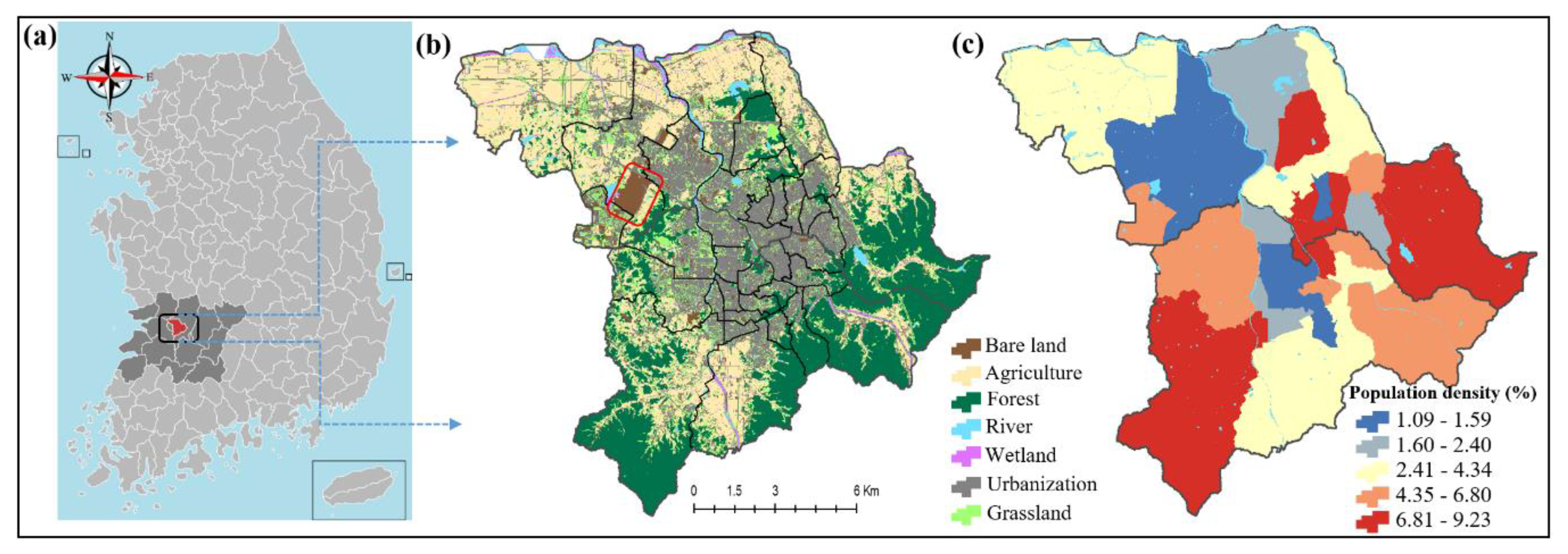
2.1.1. Study Area
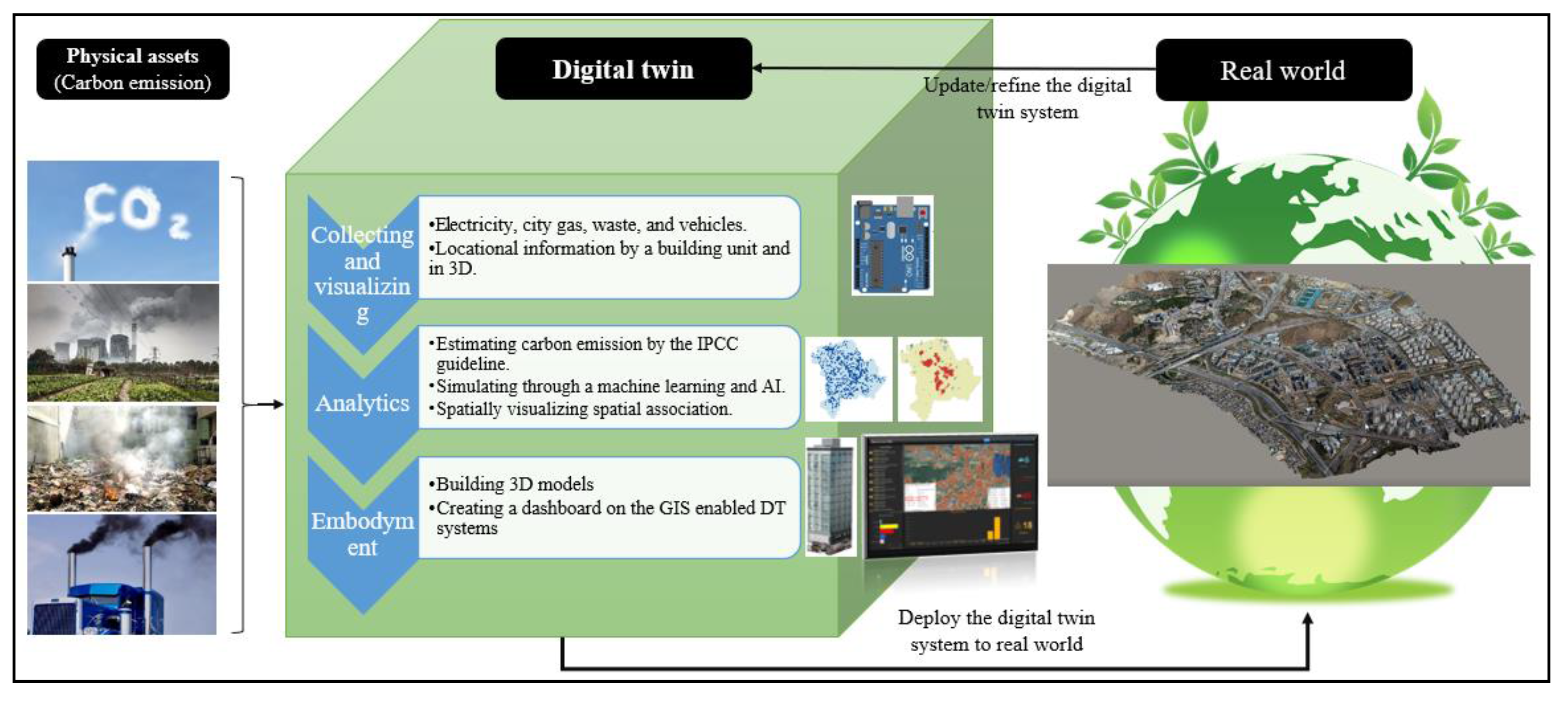
2.1.2. Developing a Schematic Diagram and Data Collection
2.2. Methodology
2.2.1. Quantifying the Four Indicators
2.2.2. Analysis Step: Visualization and Simulation
2.2.3. Deployment Step: GIS-Enabled DT System
3. Results
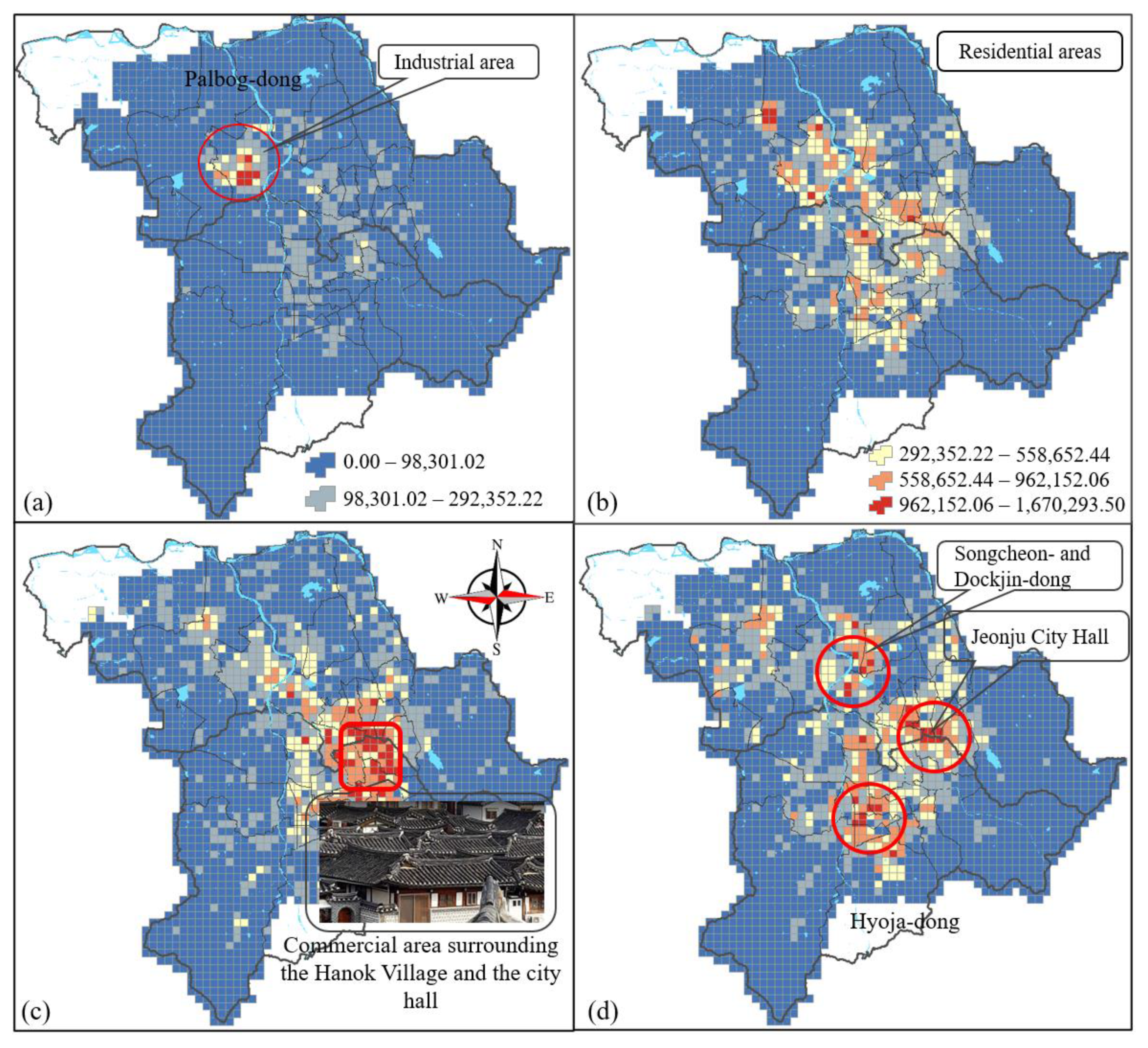
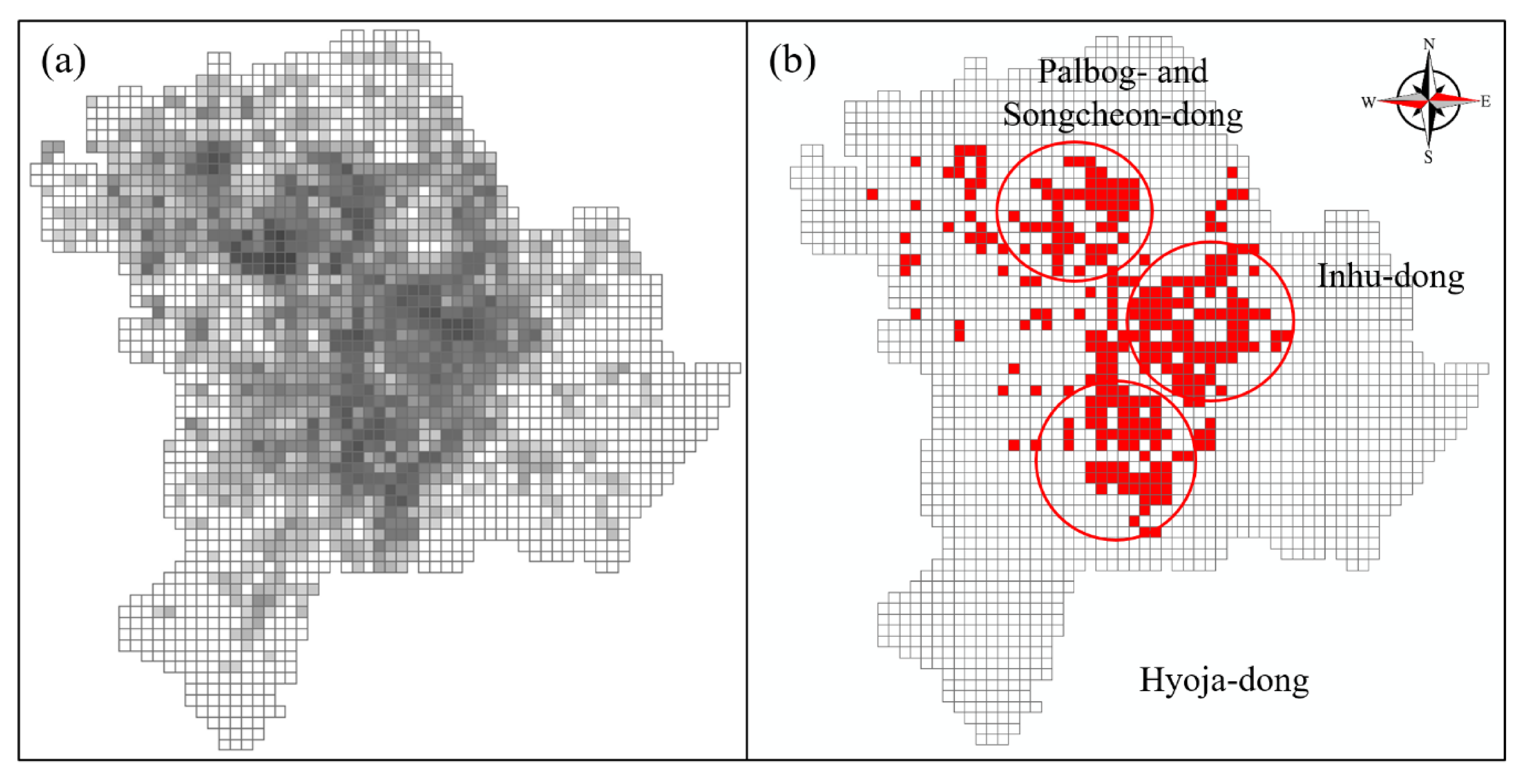
3.1. Mapping Carbon Emissions by the Primary Four Factors
3.2. Predicting Simulation Results of Machine Learning Techniques
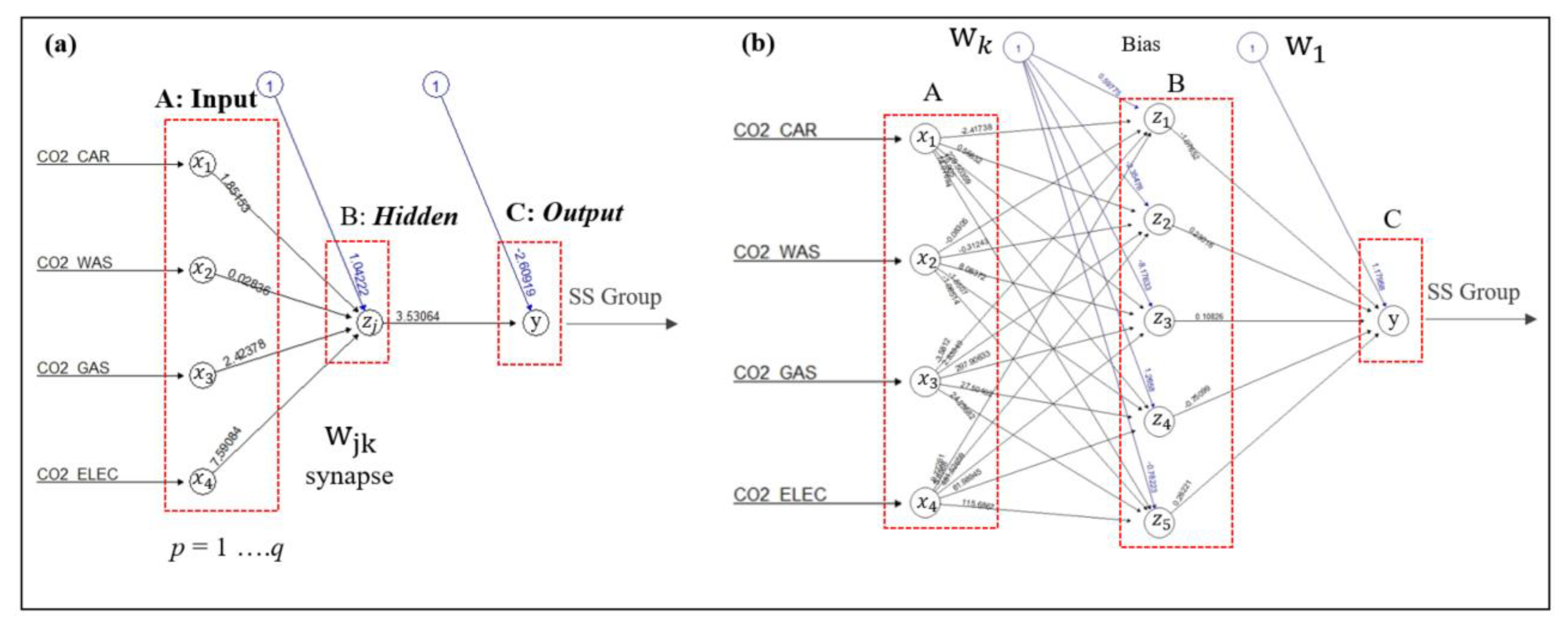
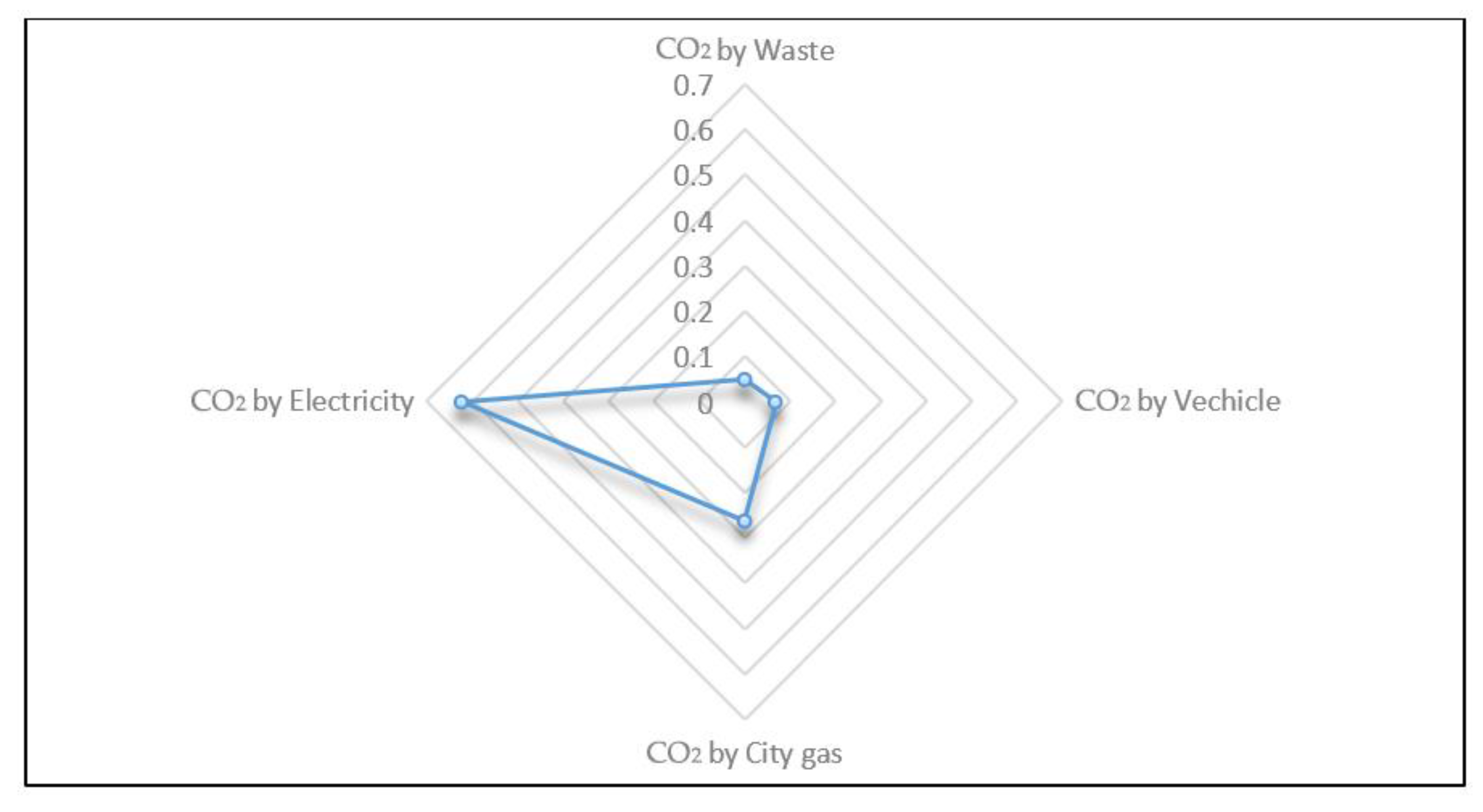
3.3. Influence Analysis of Factors Using ANN
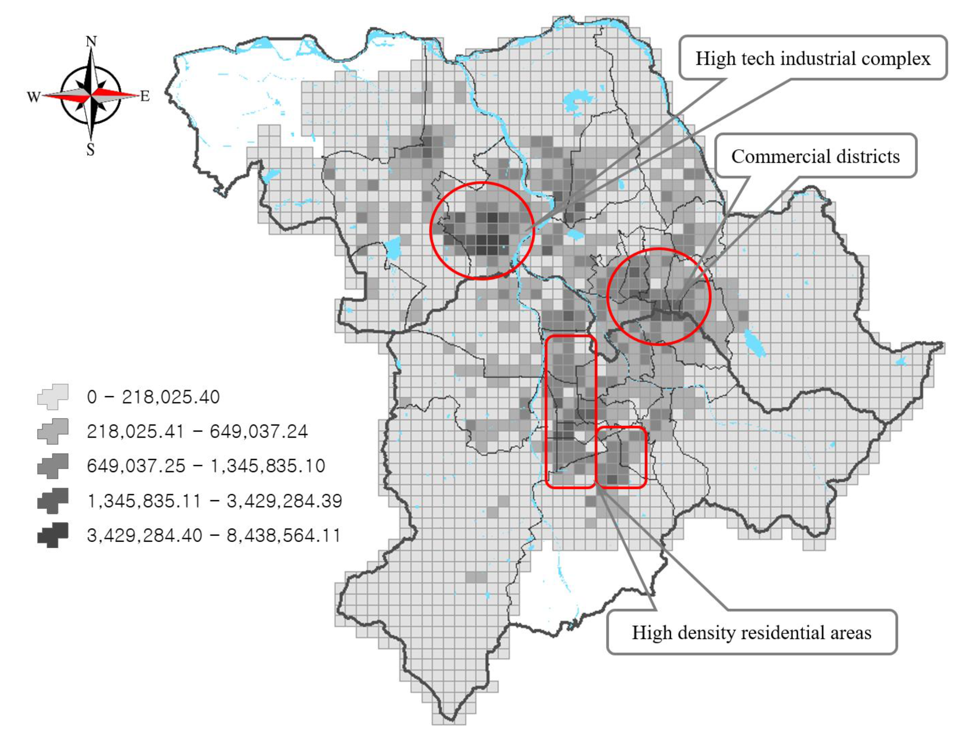
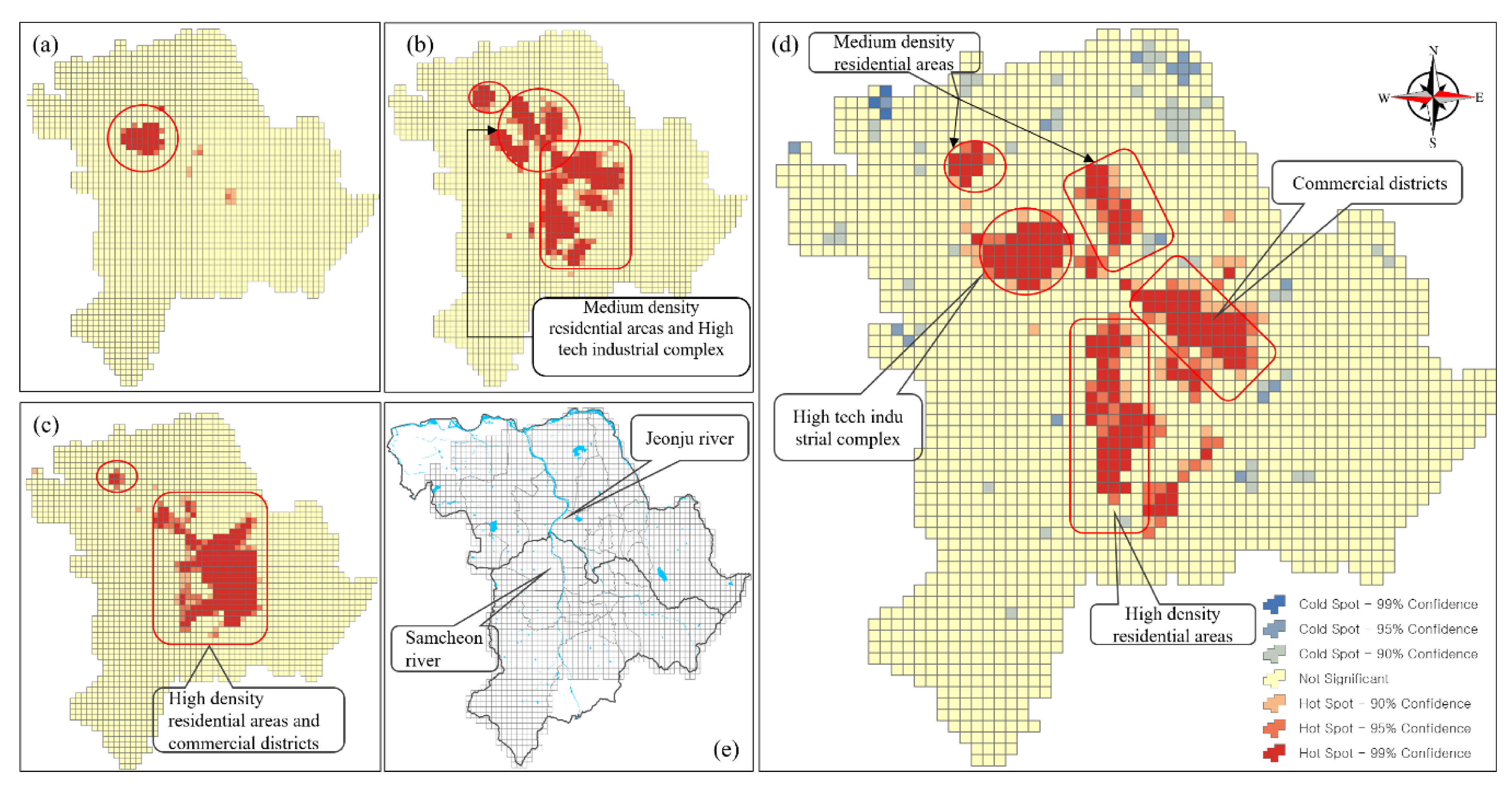
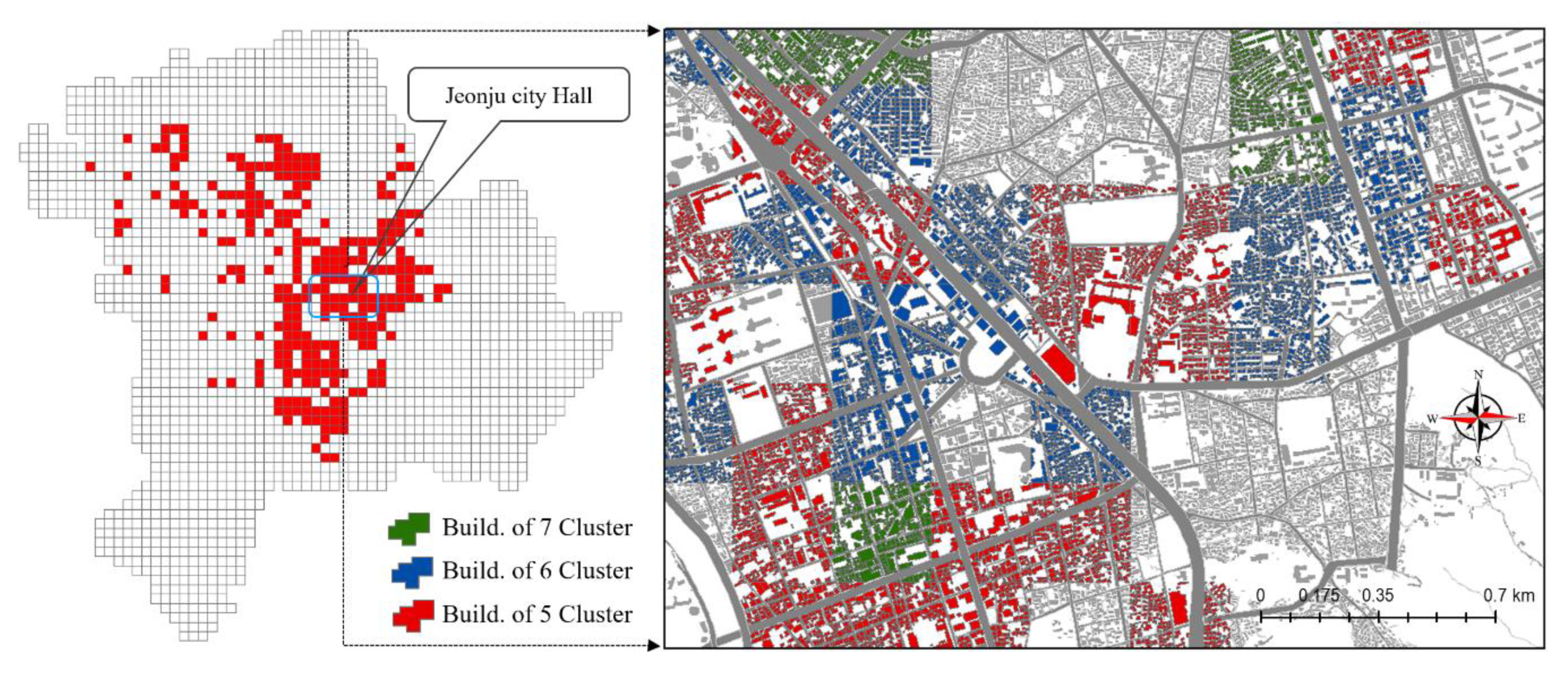
3.4. Visualizing Spatial Association among the Four Factors
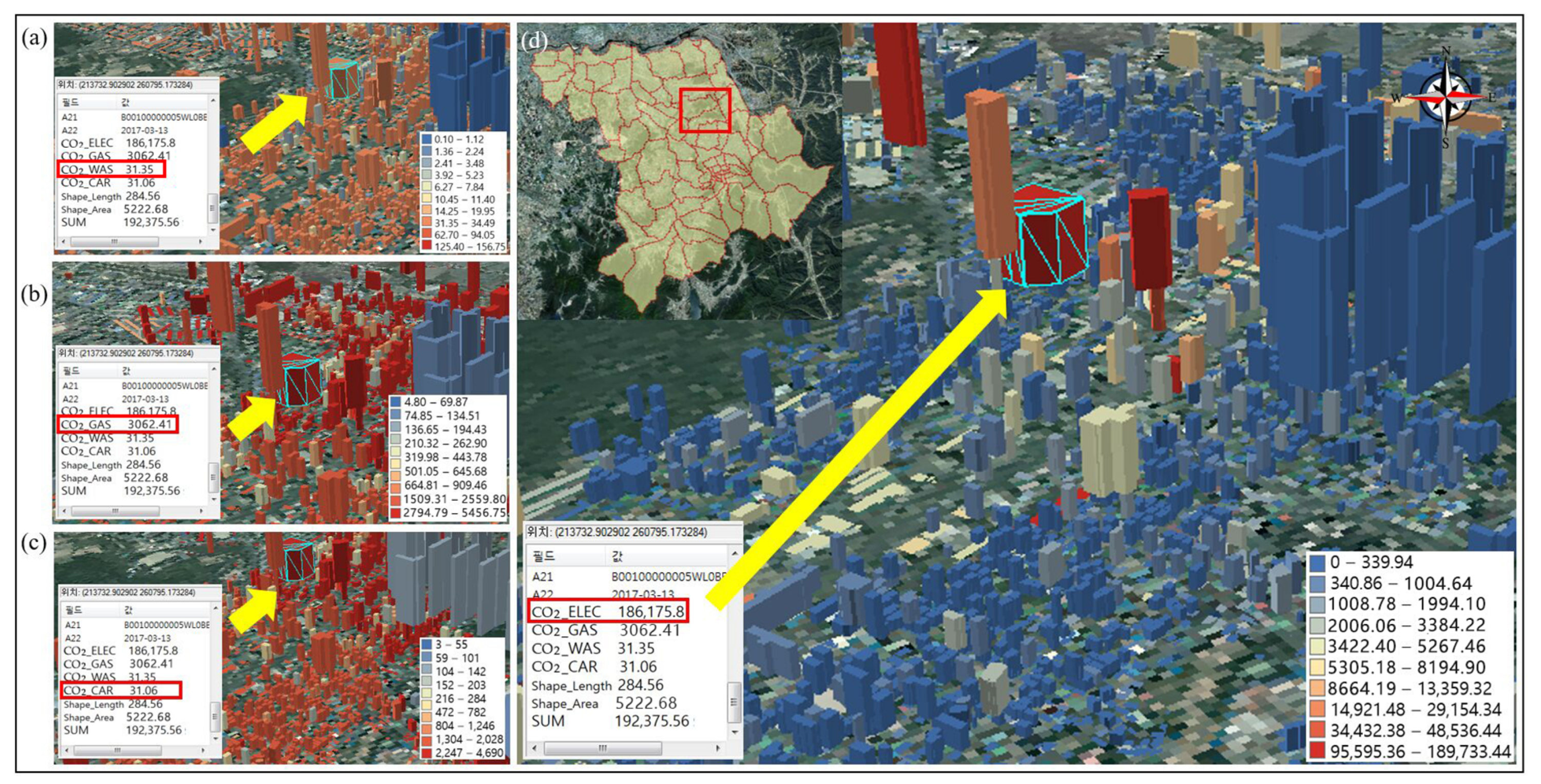
3.5. Deploying a GIS-Enabled DT System for Carbon Emissions
4. Discussion
5. Conclusions
Author Contributions
Funding
Acknowledgments
Conflicts of Interest
References
- Grieves, M. Digital twin: Manufacturing excellence through virtual factory replication. White Paper 2014, 1, 1–7. [Google Scholar]
- Schrotter, G.; Hürzeler, C. The Digital Twin of the City of Zurich for Urban Planning. PFG J. Photogramm. Remote Sens. Geoinf. Sci. 2020, 1–14. [Google Scholar] [CrossRef]
- Sepasgozar, S.M.; Hawken, S.; Sargolzaei, S.; Foroozanfa, M. Implementing citizen centric technology in developing smart cities: A model for predicting the acceptance of urban technologies. Technol. Forecast. Soc. Chang. 2019, 142, 105–116. [Google Scholar] [CrossRef]
- Richter, A.; Löwner, M.O.; Ebendt, R.; Scholz, M. Towards an integrated urban development considering novel intelligent transportation systems: Urban Development Considering Novel Transport. Technol. Forecast. Soc. Chang. 2020, 155, 119970. [Google Scholar] [CrossRef]
- Washburn, D.; Sindhu, U.; Balaouras, S.; Dines, R.A.; Hayes, N.M.; Nelson, L.E. Helping CIOs Understand “Smart City” Initiatives: Defining the Smart city, Its Drivers, and the Role of the CIO; Forrester Research, Inc.: Cambridge, MA, USA, 2010. [Google Scholar]
- Intergovernmental Panel on Climate Change [IPCC]. Global Warming of 1.5 °C: An IPCC Special Report on the Impacts of Global Warming of 1.5 °C above Pre-Industrial Levels and Related Global Greenhouse Gas Emission Pathways, in the Context of Strengthening the Global Response to the Threat of Climate Change, Sustainable Development, and Efforts to Eradicate Poverty; IPCC: Geneva, Switzerland, 2018. [Google Scholar]
- Jain, R.K.; Smith, K.M.; Culligan, P.J.; Taylor, J.E. Forecasting energy consumption of multi-family residential buildings using support vector regression: Investigating the impact of temporal and spatial monitoring granularity on performance accuracy. Appl. Energy 2014, 123, 168–178. [Google Scholar] [CrossRef]
- Stocker, T.F.; Qin, D.; Plattner, G.-K.; Alexander, L.-V.; Allen, S.K.; Bindoff, N.L.; Bréon, F.-M.; Church, J.A.; Cubasch, U.; Emori, S.; et al. Technical Summary. In Climate Change 2013: The Physical Science Basis. Contribution of Working Group I to the Fifth Assessment Report of the Intergovernmental Panel on Climate Change; Stocker, T.F., Qin, D., Plattner, G.-K., Tignor, M., Allen, S.K., Boschung, J., Nauels, A., Xia, Y., Bex, V., Midgley, P.M., Eds.; Cambridge University Press: Cambridge, UK; New York, NY, USA, 2013; pp. 33–115. [Google Scholar]
- Ruiz-Guerra, I.; Molina-Moreno, V.; Cortés-García, F.J.; Núñez-Cacho, P. Prediction of the impact on air quality of the cities receiving cruise tourism: The case of the Port of Barcelona. Heliyon 2019, 5, e01280. [Google Scholar] [CrossRef]
- Górecki, J.; Núñez-Cacho, P.; Corpas-Iglesias, F.A.; Molina, V. How to convince players in construction market? Strategies for effective implementation of circular economy in construction sector. Cogent Eng. 2019, 6, 1690760. [Google Scholar] [CrossRef]
- The Carbon Brief Profile: South Korea. Available online: https://www.carbonbrief.org/the-carbon-brief-profile-south-korea (accessed on 10 December 2019).
- Shafto, M.; Conroy, M.; Doyle, R.; Glaessgen, E. Modeling, Simulation, Information Technology and Processing Roadmap. Technol. Area 2012, 1–33. Available online: https://www.nasa.gov/sites/default/files/501321main_TA11-ID_rev4_NRC-wTASR.pdf (accessed on 2 November 2020).
- Tuegel, E.J.; Ingraffea, A.R.; Eason, T.G.; Spottswood, S.M. Reengineering aircraft structural life prediction using a digital twin. Int. J. Aerosp. Eng. 2011, 2011, 1–14. [Google Scholar] [CrossRef]
- Glaessgen, E.; Stargel, D. The digital twin paradigm for future NASA and US air force vehicles. In Proceedings of the AAIA 53rd Structures, Structural Dynamics, and Materials Conference, Honolulu, HI, USA, 23–26 April 2012; pp. 1–14. [Google Scholar]
- Cerrone, A.; Hochhalter, J.; Heber, G.; Ingraffea, A. On the effects of modeling as-manufactured geometry: Toward digital twin. Int. J. Aerosp. Eng. 2014, 2014, 1–10. [Google Scholar] [CrossRef]
- Söderberg, R.; Wärmefjord, K.; Carlson, J.S.; Lindkvist, L. Toward a digital twin for real-time geometry assurance in individualized production. CIRP Ann. 2017, 66, 137–140. [Google Scholar] [CrossRef]
- Erkoyuncu, J.A.; Butala, P.; Roy, R. Digital twins: Understanding the added value of integrated models for through-life engineering services. Procedia Manuf. 2018, 16, 139–146. [Google Scholar]
- Grieves, M.; Vickers, J. Digital twin: Mitigating unpredictable, undesirable emergent behavior in complex systems. In Transdisciplinary Perspectives on Complex Systems; Kahlen, F.J., Flumerfelt, S., Alves, A., Eds.; Springer: Cham, Switzerland, 2017; pp. 85–113. [Google Scholar]
- Alam, K.M.; El Saddik, A. C2PS: A digital twin architecture reference model for the cloud-based cyber-physical systems. IEEE Access 2017, 5, 2050–2062. [Google Scholar] [CrossRef]
- Schleich, B.; Anwer, N.; Mathieu, L.; Wartzack, S. Shaping the digital twin for design and production engineering. CIRP Ann. 2017, 66, 141–144. [Google Scholar] [CrossRef]
- Wagner, R.; Schleich, B.; Haefner, B.; Kuhnle, A.; Wartzack, S.; Lanza, G. Challenges and potentials of digital twins and Industry 4.0 in product design and production for high performance products. Procedia CIRP 2019, 84, 88–93. [Google Scholar] [CrossRef]
- Ambra, T.; Caris, A.; Macharis, C. The Digital Twin concept and its role in reducing uncertainty in synchromodal transport. In Proceedings of the IPIC 2019, 6th International Physical Internet Conference, London, UK, 8 July 2019. [Google Scholar]
- Li, D.; Shen, X.; Yu, Y.; Guan, H.; Li, J.; Zhang, G.; Li, D. Building Extraction from Airborne Multi-Spectral LiDAR Point Clouds Based on Graph Geometric Moments Convolutional Neural Networks. Remote Sens. 2020, 12, 3186. [Google Scholar] [CrossRef]
- Park, J.; Cho, D.; Lee, S.; Lee, M.; Nam, H.; Yang, H. A study on the methodology of extracting the vulnerable districts of the aged welfare using artificial intelligence and geospatial information. J. Cadastre Land InformatiX 2018, 48, 169–186. [Google Scholar]
- Farin, G.; Hoschek, J.; Kim, M.S. Handbook of Computer Aided Geometric Design; Elsevier: Amsterdam, The Netherlands, 2002. [Google Scholar]
- Günther, F.; Fritsch, S. Neuralnet: Training of neural networks. R J. 2010, 2, 30–38. [Google Scholar]
- Qi, Q.; Tao, F.; Hu, T.; Anwer, N.; Liu, A.; Wei, Y.; Wang, L.; Nee, A. Enabling technologies and tools for digital twin. J. Manuf. Syst. 2019. [Google Scholar] [CrossRef]
- Shirowzhan, S.; Tan, W.; Sepasgozar, S.M. Digital Twin and CyberGIS for improving connectivity and measuring the impact of infrastructure construction planning in smart cities. ISPRS Int. J. Geo-Inf. 2020, 9, 240. [Google Scholar] [CrossRef]
- Albino, V.; Berardi, U.; Dangelico, R.M. Smart cities: Definitions, dimensions, performance, and initiatives. J. Urban Technol. 2015, 22, 3–21. [Google Scholar] [CrossRef]
- Parslow, P. ISO/IEC JTC1/WG11 (IT aspects of) Smart Cities. Presented at the Smart Cities Domain Working Group (DWG) of the 107th OGC Technical Committee, Ft. Collins, CO, USA, 4–8 June 2018. [Google Scholar]
- Digital Underground. Available online: https://digitalunderground.sg/ (accessed on 20 June 2020).
- Smart Cities Council Australia New Zealand. Digital Twin. Data Leadership Guidance Note. Available online: https://anz.smartcitiescouncil.com/system/tdf/anz_smartcitiescouncil_com/public_resources/guidance_note_digital_twin_issue.pdf?file=1&type=node&id=7255&force= (accessed on 2 November 2020).
- Geospatial Technology Trends. Available online: https://www.ogc.org/OGCTechTrends (accessed on 16 July 2020).
- UN-GGIM. Future Trends in Geospatial Information Management: The Five to Ten Year Vision, 3rd ed. (draft v1.0). Available online: https://ggim.un.org/future-trends/ (accessed on 16 July 2020).
- JeonJu’s Sustainable Development Committee (JSDC). Report for Sustainable Index Assessment; Jeonju City: Jeonju, Korea, 2018; pp. 159–226. [Google Scholar]
- Yin, X.; Hao, Y.; Yang, Z.; Zhang, L.; Su, M.; Cheng, Y.; Zhang, P.; Yang, J.; Liang, S. Changing carbon footprint of urban household consumption in Beijing: Insight from a nested input-output analysis. J. Clean. Prod. 2020, 258, 120698. [Google Scholar] [CrossRef]
- Lu, H.; Liu, G.; Miao, C.; Zhang, C.; Cui, Y.; Zhao, J. Spatial pattern of residential carbon dioxide emissions in a rapidly urbanizing Chinese city and its mismatch effect. Sustainability 2018, 10, 827. [Google Scholar] [CrossRef]
- Liu, W.; Spaargaren, G.; Heerink, N.; Mol, A.P.; Wang, C. Energy consumption practices of rural households in north China: Basic characteristics and potential for low carbon development. Energy Policy 2013, 55, 128–138. [Google Scholar] [CrossRef]
- Ministry of Environment (ME) of South Korea. Manual of the Greenhouse Gas Discharge Estimate. 2012, p. 77. Available online: http://www.me.go.kr/home/file/readDownloadFile.do?fileId=96230&fileSeq=1 (accessed on 10 September 2020).
- Kadian, R.; Dahiya, R.P.; Garg, H.P. Energy-related emissions and mitigation opportunities from the household sector in Delhi. Energy Policy 2007, 35, 6195–6211. [Google Scholar] [CrossRef]
- Lee, S.; Lee, B. The influence of urban form on GHG emissions in the US household sector. Energy Policy 2014, 68, 534–549. [Google Scholar] [CrossRef]
- Sanches-Pereira, A.; Tudeschini, L.G.; Coelho, S.T. Evolution of the Brazilian residential carbon footprint based on direct energy consumption. Renew. Sustain. Energy Rev. 2016, 54, 184–201. [Google Scholar] [CrossRef]
- Björkman, M.; Holmström, K. Global optimization of costly nonconvex functions using radial basis functions. Optim. Eng. 2000, 1, 373–397. [Google Scholar] [CrossRef]
- Hinton, G.E.; McClelland, J.L.; Rumelhart, D.E.; Rnmelhart, D.E. Parallel Distributed Processing: Explorations in the Microstructure of Cognition; MIT Press: Cambridge, MA, USA, 1986. [Google Scholar]
- Yang, B. GIS crime mapping to support evidence-based solutions provided by community-based organizations. Sustainability 2019, 11, 4889. [Google Scholar] [CrossRef]
- Hwang, C.S.; Hong, S.Y.; Hwang, T.; Yang, B. Strengthening the statistical summaries of economic output areas for urban planning support systems. Sustainability 2020, 12, 5640. [Google Scholar] [CrossRef]
- Park, J.; Kim, J.; Yang, B. Spatializing an artist-resident community area at a building-level: A case study of Garosu-gil, South Korea. Sustainability 2020, 12, 6116. [Google Scholar] [CrossRef]
- Anselin, L. Local indicators of spatial association—LISA. Geogr. Anal. 1995, 27, 93–115. [Google Scholar] [CrossRef]
- Resch, B.; Puetz, I.; Bluemke, M.; Kyriakou, K.; Miksch, J. An Interdisciplinary Mixed-Methods Approach to Analyzing Urban Spaces: The Case of Urban Walkability and Bikeability. Int. J. Environ. Res. Public Health 2020, 17, 6994. [Google Scholar] [CrossRef]
- Lee, J.; Yang, B. Developing an optimized texture mapping for photorealistic 3D buildings. Trans. GIS 2019, 23, 1–21. [Google Scholar] [CrossRef]
- Yang, B. Developing a mobile mapping system for 3D GIS and smart city planning. Sustainability 2019, 11, 3713. [Google Scholar] [CrossRef]
- Ross, D.I.L. Virtual 3D City Models in Urban Land Management. Doctoral Dissertation, Technischen Universitat, Berlin, Germany, 2010. [Google Scholar]
- Open Geospatial Consortium [OGC]. OGC City Geography Markup Language (CityGML) En-Coding Standard; Open Geospatial Consortium: Wayland, MA, USA, 2012. [Google Scholar]


| Indicators | Equations in Accordance with the Intergovernmental Panel on Climate Change (IPCC) Guideline | Sources |
|---|---|---|
| Electricity usage (Month) | Electricity energy consumption (1 Mwh) × carbon emission factor (0.460) | Energy conversion division of Jeonju city |
| City gas consumption (Month) | Energy consumption × carbon emission factor × combustion rate × carbon conversion factor (44/12) | Household gas company |
| Household waste (Month) | Total waste x dry content x carbon fraction (CF) × Fossil carbon fraction (FCF) Oxidation coefficient × carbon conversion factor (44/12) | Resource circulation division of Jeonju city |
| Number of vehicles (Year) | Average daily mileage by type of car × emission factor by vehicle type | Transportation division of Jeonju city |
| Carbon Emission | Mean | SD | Max | Min |
|---|---|---|---|---|
| By electricity | 51,834.8 | 327,807.2 | 8,189,923.5 | 0.001 |
| By city gas | 27,353.4 | 59,159.8 | 786,394.9 | 0 |
| By household waste | 1113.5 | 2039.8 | 14,052.9 | 0.002 |
| By the number of vehicles | 121,488.5 | 215,419.8 | 1,670,293.5 | 0.132 |
| Cluster | Predictive Variables by Cluster | ||||||||||
|---|---|---|---|---|---|---|---|---|---|---|---|
| 1 | 2 | 3 | 4 | 5 | 6 | 7 | 8 | 9 | 10 | Accuracy | |
| 1 | 359 | 836 | 7 | 4 | - | - | - | - | - | - | 29.8% |
| 2 | - | 8 | 253 | 39 | 11 | - | - | - | - | - | 2.7% |
| 3 | - | - | - | 148 | 33 | - | - | - | - | - | 0.0% |
| 4 | - | - | - | - | 137 | - | - | - | - | - | 0.0% |
| 5 | - | - | - | - | 115 | - | - | - | - | - | 100.0% |
| 6 | - | - | - | - | 31 | 68 | - | - | - | - | 68.7% |
| 7 | - | - | - | - | 16 | - | 57 | - | - | - | 78.1% |
| 8 | - | - | - | - | 17 | - | 38 | - | - | - | 0.0% |
| 9 | - | - | - | - | 6 | - | 17 | - | - | - | 0.0% |
| 10 | - | - | - | - | 1 | 0 | 6 | - | - | - | 0.0% |
| Z1 | Z2 | Z3 | Z4 | Z5 | |
|---|---|---|---|---|---|
| Bias 1 | 0.996 | −2.338 | −0.526 | 0.582 | −3.685 |
| CO2 CAR (x1) | −0.018 | 0.495 | 9.075 | −0.429 | 5.188 |
| CO2 WAS (x2) | −0.031 | −0.889 | 0.391 | 0.0390 | −0.090 |
| CO2 GAS (x3) | −1.081 | 1.973 | 19.436 | 2.872 | 12.820 |
| CO2 ELEC (x4) | −4.568 | −1.478 | 66.844 | 7.334 | 34.710 |
| Bias 2 | Z1 | Z2 | Z3 | Z4 | Z5 | |
|---|---|---|---|---|---|---|
| SS Group (y) | 1.250 | −1.142 | 0.707 | 0.481 | −1.050 | 0.394 |
| Clusters | Electricity | City Gas | Household Waste | Vehicle | #s of Building | ||||||||||||
|---|---|---|---|---|---|---|---|---|---|---|---|---|---|---|---|---|---|
| Mean | Max | Min | SD | Mean | Max | Min | SD | Mean | Max | Min | SD | Mean | Max | Min | SD | ||
| 5 | 94,508.4 | 425,765 | 2019.1 | 75,014.8 | 96,636 | 342,563.6 | 5.9 | 54,476.3 | 5200.4 | 11,451.3 | 276.1 | 2906.4 | 364,555.5 | 563,995.5 | 49,195.8 | 95,570 | 17,746 |
| 6 | 129,463.9 | 674,482.3 | 2390.5 | 120,654.9 | 125,558.6 | 461,273.3 | 27,448.5 | 56,118.1 | 5906.3 | 12,390.2 | 816.6 | 3425.3 | 3487.9 | 36,453 | 17 | 3005.3 | 18,715 |
| 7 | 168,640.5 | 991,836.6 | 27,310.1 | 188,558.6 | 185,434.5 | 599,505.6 | 44,594.4 | 73,958.4 | 5410.1 | 11,381.4 | 883.4 | 2334.8 | 773,562.9 | 1,069,540 | 157,701.2 | 200,251.8 | 11,052 |
Publisher’s Note: MDPI stays neutral with regard to jurisdictional claims in published maps and institutional affiliations. |
© 2020 by the authors. Licensee MDPI, Basel, Switzerland. This article is an open access article distributed under the terms and conditions of the Creative Commons Attribution (CC BY) license (http://creativecommons.org/licenses/by/4.0/).
Share and Cite
Park, J.; Yang, B. GIS-Enabled Digital Twin System for Sustainable Evaluation of Carbon Emissions: A Case Study of Jeonju City, South Korea. Sustainability 2020, 12, 9186. https://doi.org/10.3390/su12219186
Park J, Yang B. GIS-Enabled Digital Twin System for Sustainable Evaluation of Carbon Emissions: A Case Study of Jeonju City, South Korea. Sustainability. 2020; 12(21):9186. https://doi.org/10.3390/su12219186
Chicago/Turabian StylePark, Jiman, and Byungyun Yang. 2020. "GIS-Enabled Digital Twin System for Sustainable Evaluation of Carbon Emissions: A Case Study of Jeonju City, South Korea" Sustainability 12, no. 21: 9186. https://doi.org/10.3390/su12219186
APA StylePark, J., & Yang, B. (2020). GIS-Enabled Digital Twin System for Sustainable Evaluation of Carbon Emissions: A Case Study of Jeonju City, South Korea. Sustainability, 12(21), 9186. https://doi.org/10.3390/su12219186