
Comparison of Projection in Meteorological and Hydrological Droughts in the Cheongmicheon Watershed for RCP4.5 and SSP2-4.5


 ,
,  ,
,  and
and 
Abstract
1. Introduction
2. Methodology
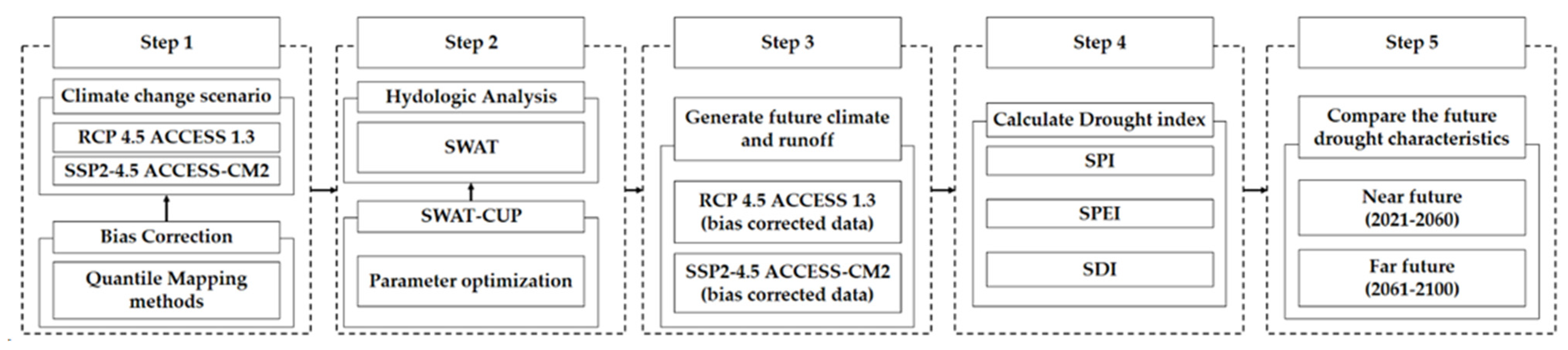
2.1. Study Procedure
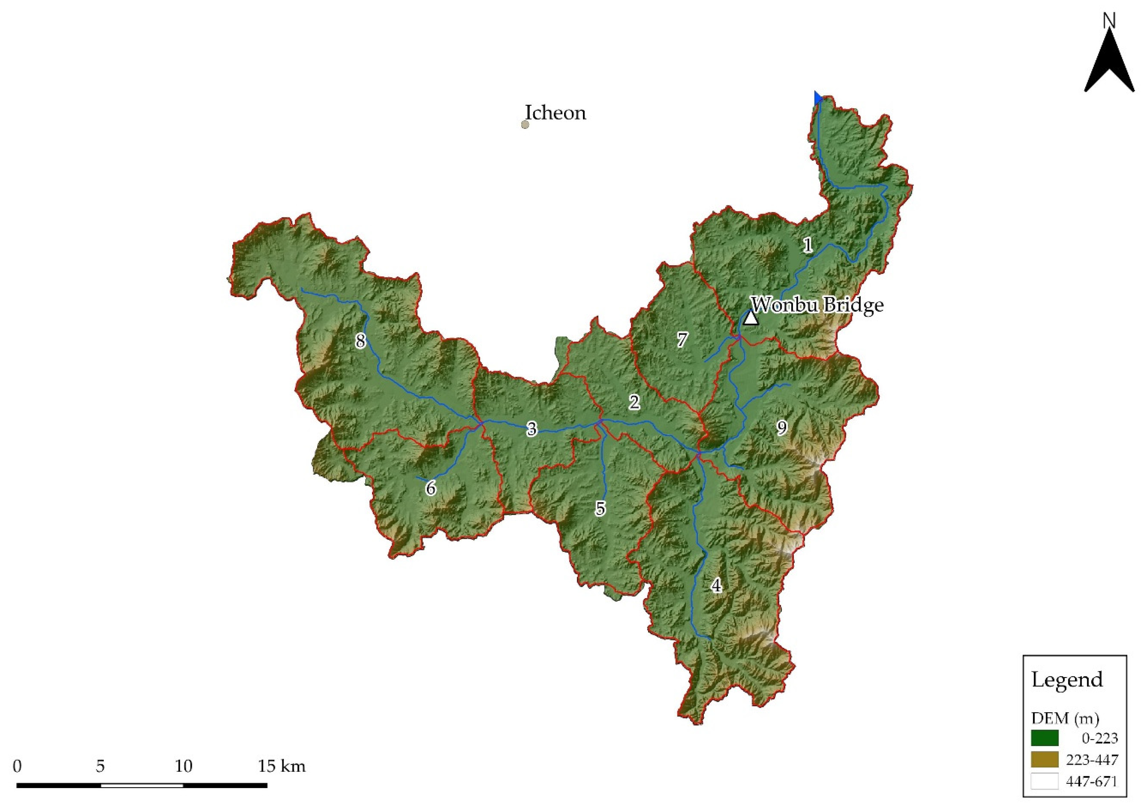
2.2. Study Area and Datasets
2.3. GCMs and Future Climate Change Scenarios
2.4. Quantile Mapping Method
2.5. SWAT and SWAT-CUP
2.6. Drought Index
2.6.1. Meteorological Drought Index
2.6.2. Hydrological Drought Index
3. Result
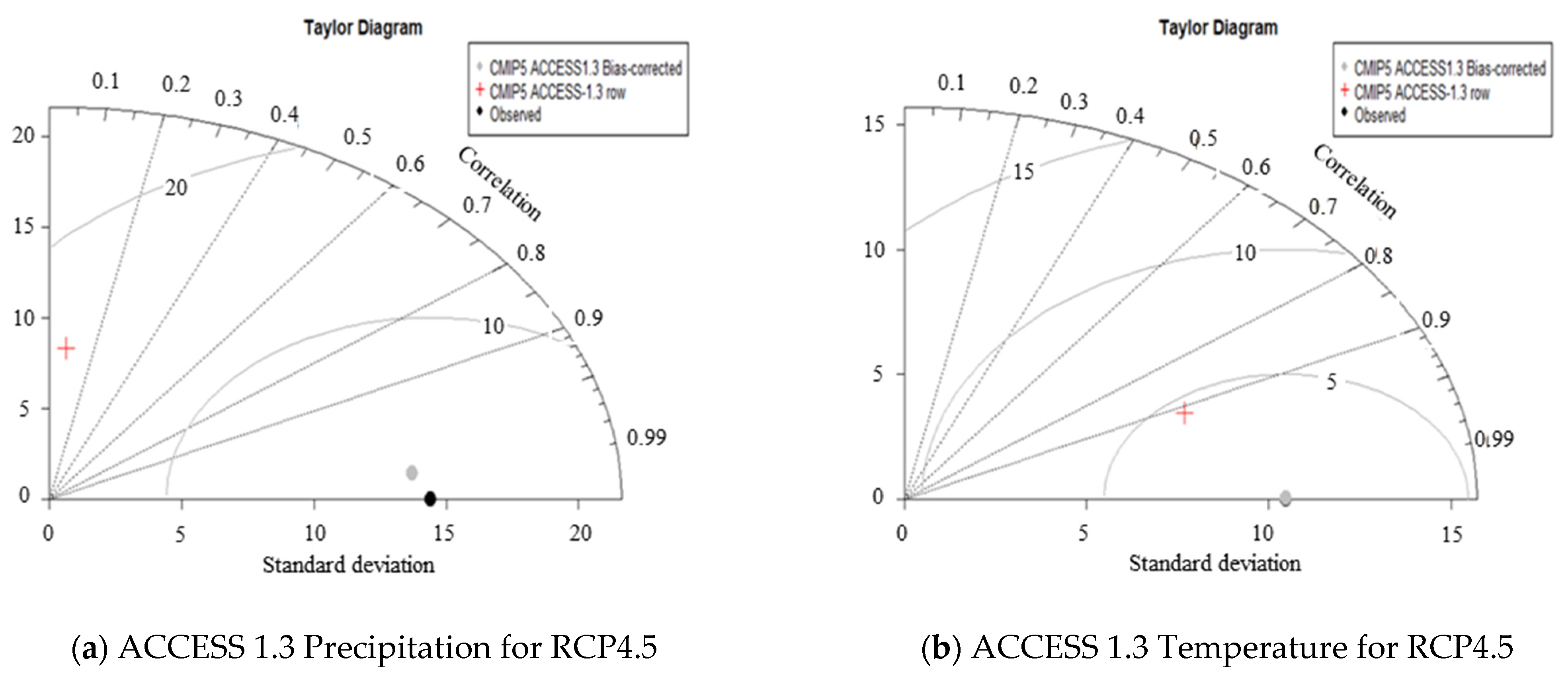
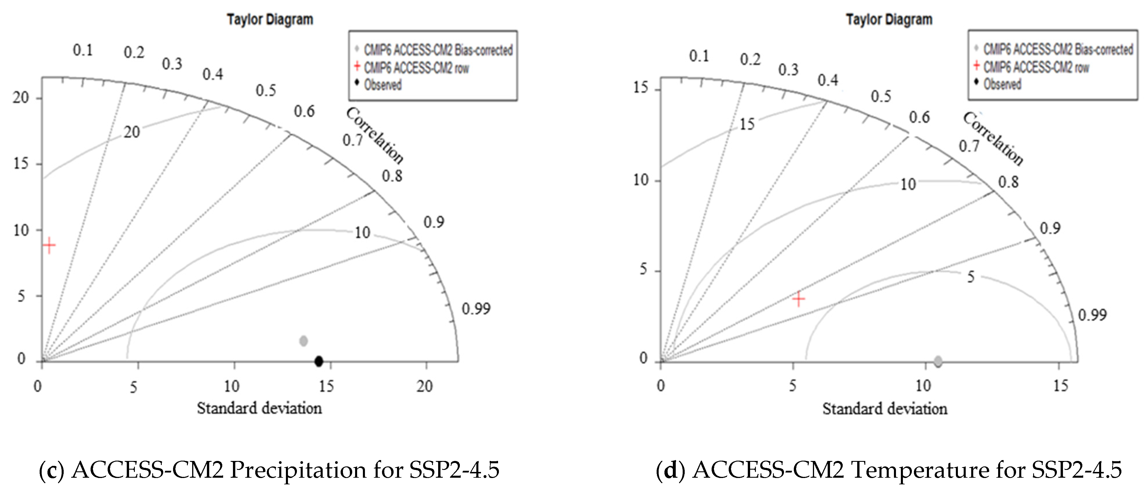
3.1. Step 1: Quantile Mapping Result
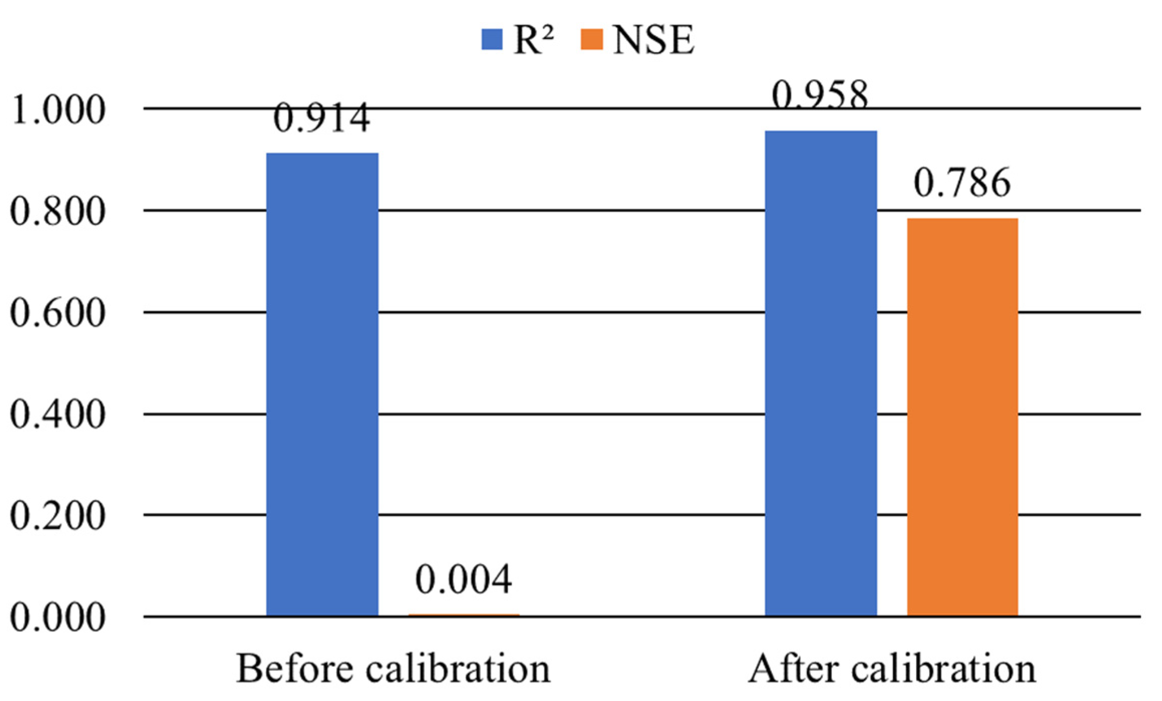
3.2. Step 2: SWAT Formulation
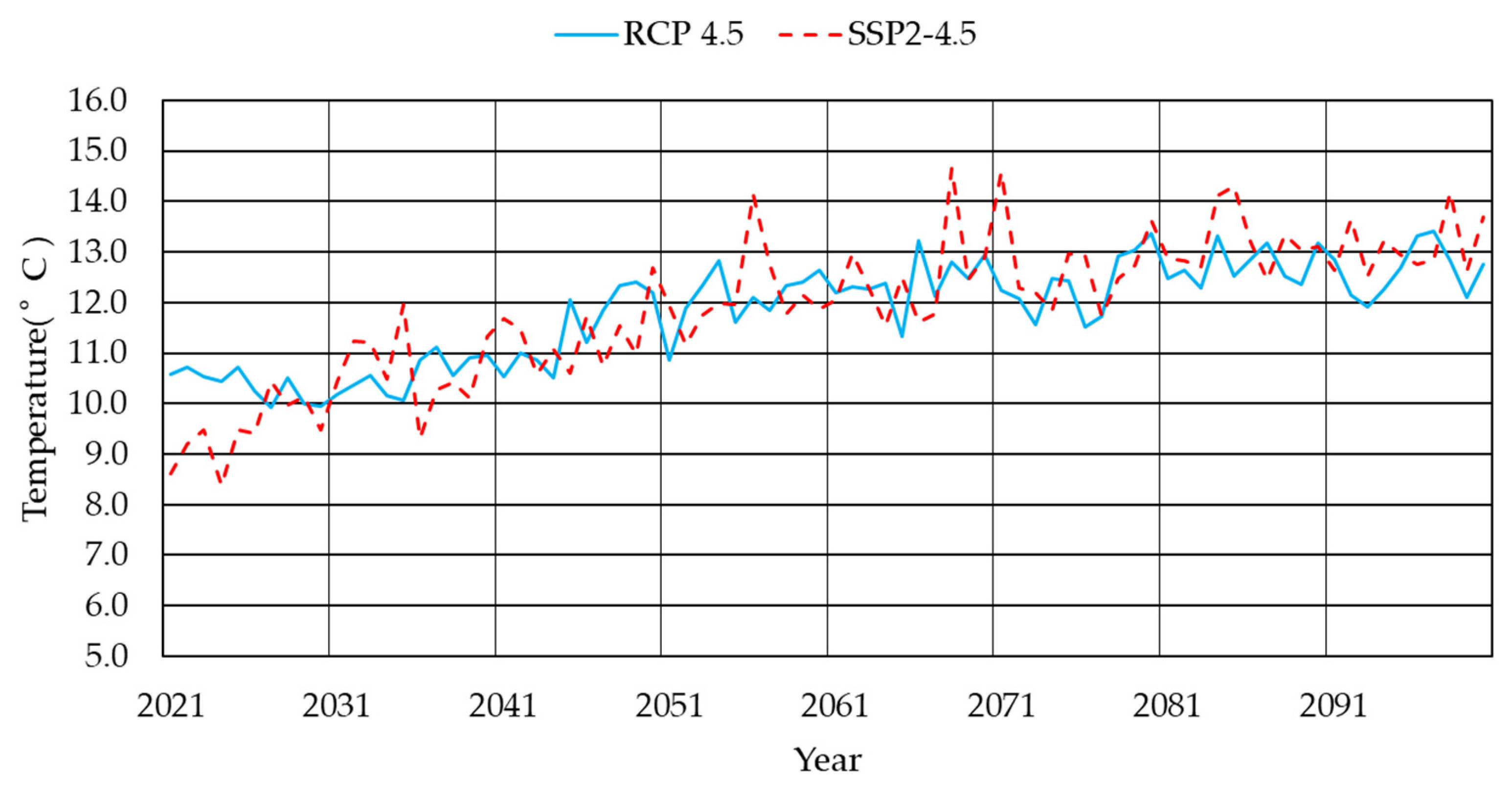
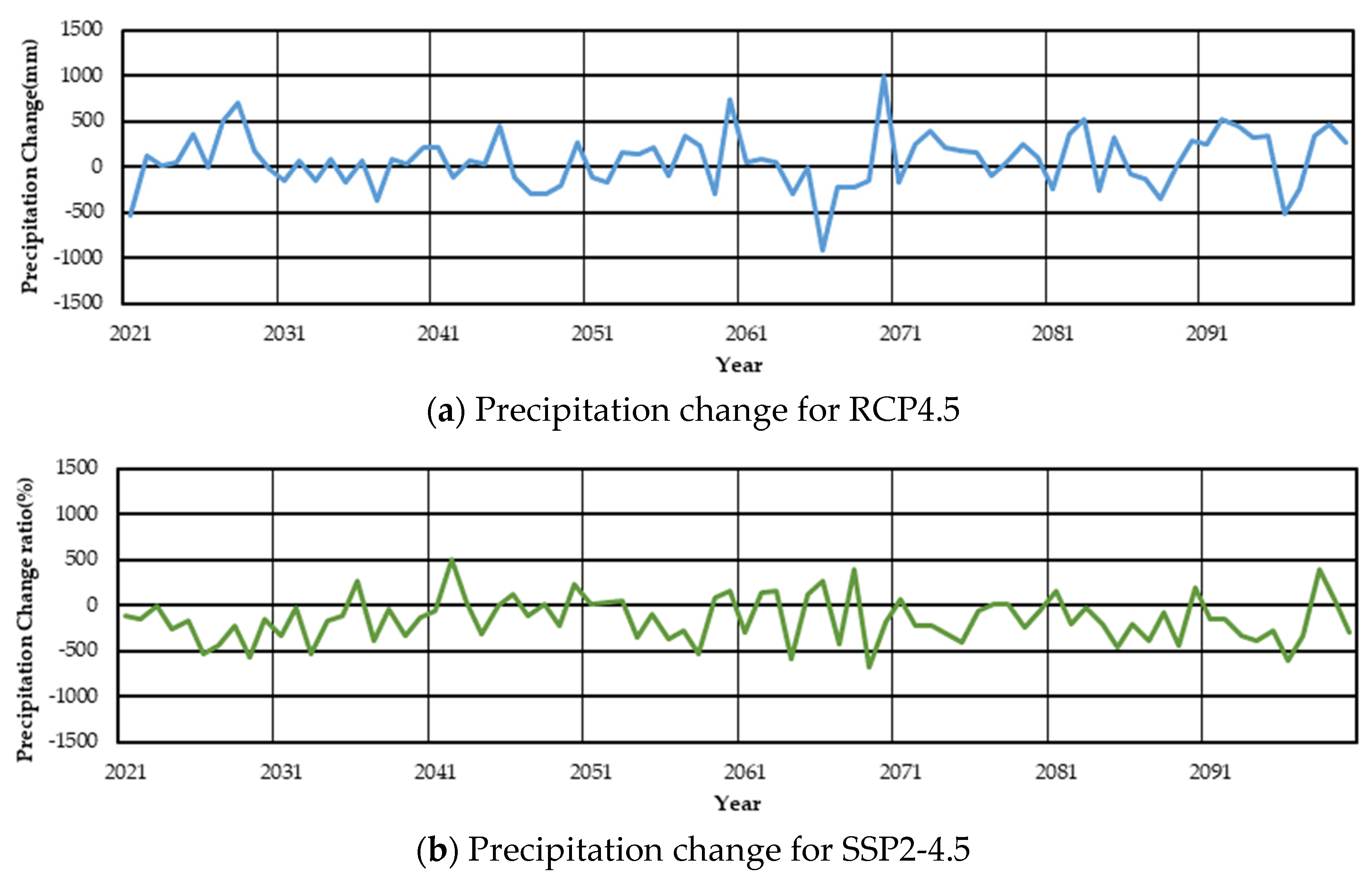
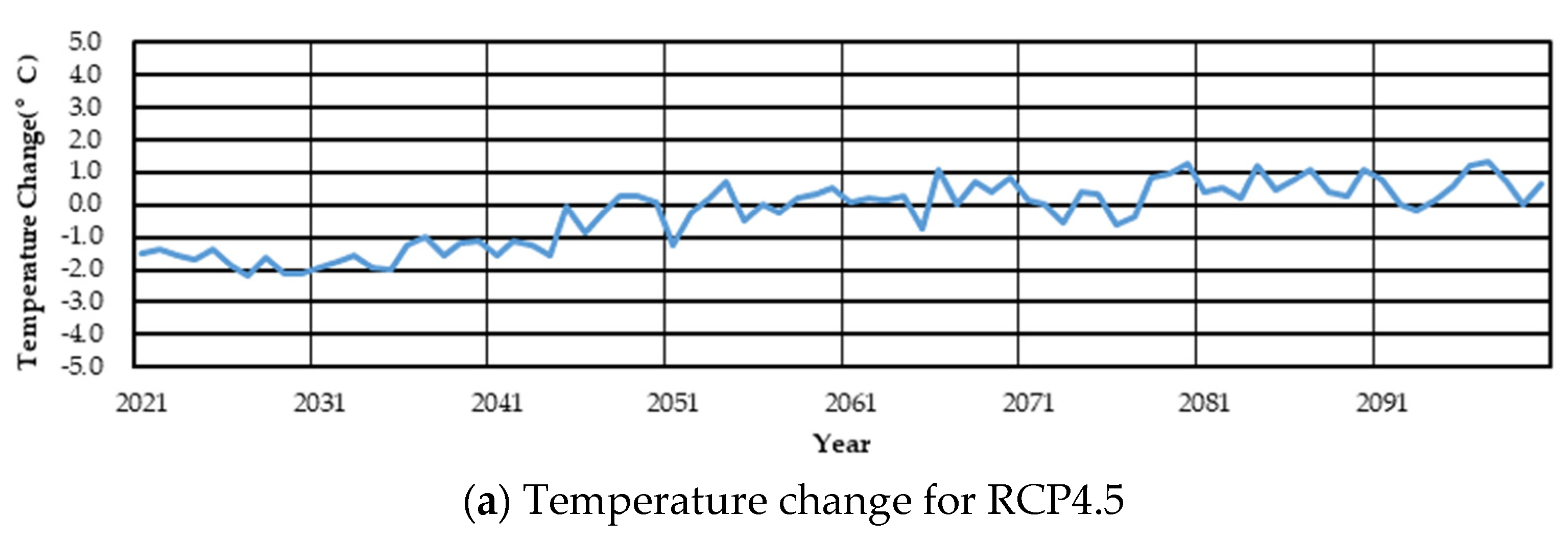
3.3. Step 3: Generation of Climate Variables and Runoff
3.4. Step 4: Calculation of Drought Index
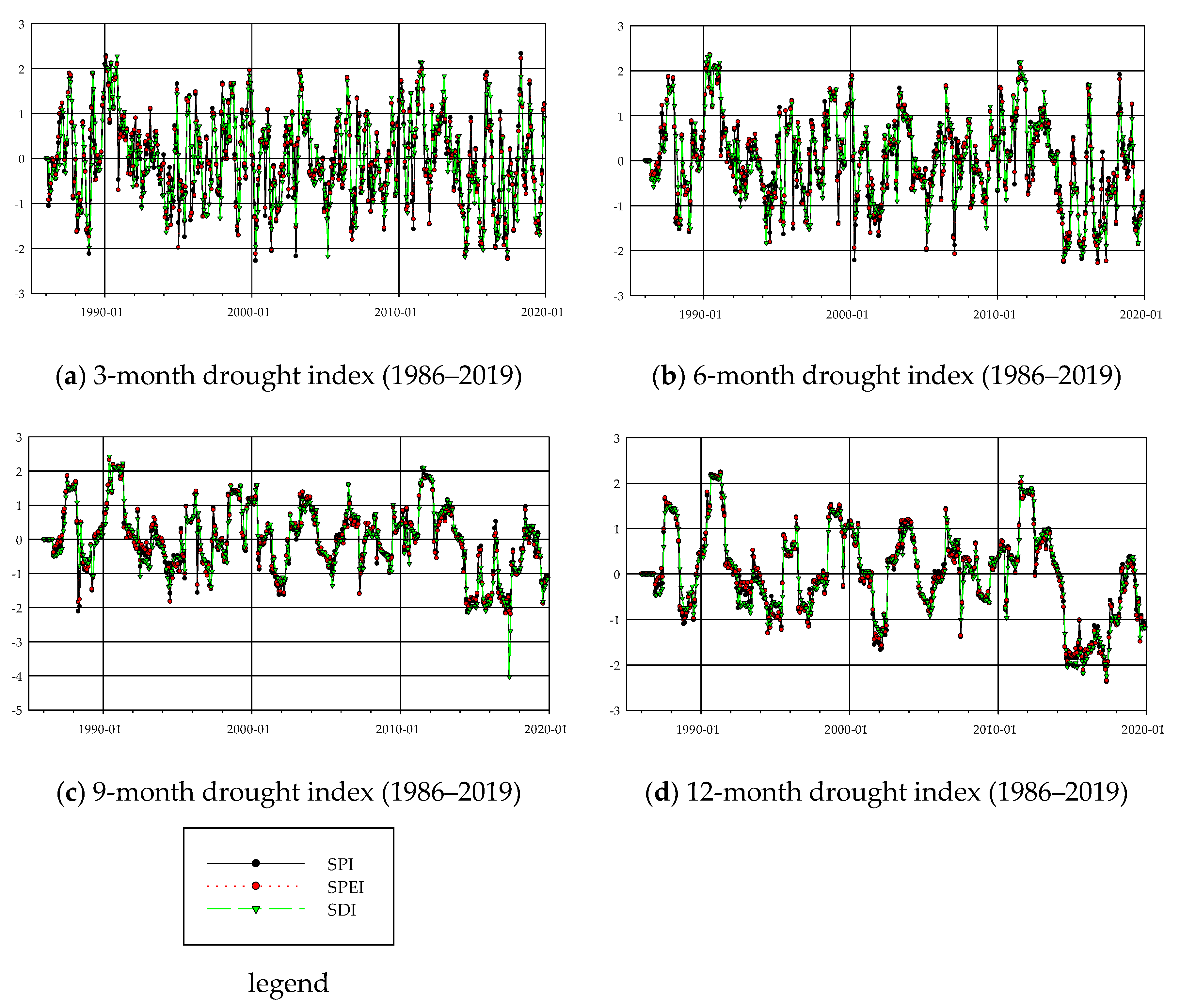
3.4.1. Historical Drought
3.4.2. Future Drought
3.5. Step 5: Comparison of Future Drought Characteristics
3.5.1. Drought Occurrence and Severity
3.5.2. The Longest Drought Period
4. Conclusions
Author Contributions
Funding
Institutional Review Board Statement
Informed Consent Statement
Data Availability Statement
Conflicts of Interest
References
- Stocker, T.F.; Qin, D.; Plattner, G.-K.; Tignor, M.; Allen, S.K.; Boschung, J.; Nauels, A.; Xia, Y.; Bex, V.; Midgley, P.M. Climate Change 2013. The Physical Science Basis; Working Group I Contribution to the Fifth Assessment Report of the Intergovernmental Panel on Climate Change-Abstract for Decision-makers; (Changements climatiques 2013. Les elements scientifiques; Contribution du groupe de travail I au cinquieme rapport d’evaluation du groupe d’experts intergouvernemental sur l’evolution du CLIMAT-Resume a l’intention des décideurs); IPCC: Geneva, Switzerland, 2013. [Google Scholar]
- Shiru, M.S.; Shahid, S.; Alias, N.; Chung, E.-S. Trend Analysis of Droughts during Crop Growing Seasons of Nigeria. Sustainability 2018, 10, 871. [Google Scholar] [CrossRef]
- Arnell, N.W.; Gosling, S.N. The impacts of climate change on river flood risk at the global scale. Clim. Chang. 2016, 134, 387–401. [Google Scholar] [CrossRef]
- Khan, N.; Shahid, S.; Ismail, T.; Ahmed, K.; Nawaz, N. Trends in heat wave related indices in Pakistan. Stoch. Environ. Res. Risk Assess. 2019, 33, 287–302. [Google Scholar] [CrossRef]
- Mishra, A.K.; Singh, V.P. A review of drought concepts. J. Hydrol. 2010, 391, 202–216. [Google Scholar] [CrossRef]
- Freire-González, J.; Decker, C.; Hall, J.W. The Economic Impacts of Droughts: A Framework for Analysis. Ecol. Econ. 2017, 132, 196–204. [Google Scholar] [CrossRef]
- National-Centers-for-Environmental-Information (NCEI), U.S. Billion-dollar Weather and Climate Disasters. Available online: https://www.ncdc.noaa.gov/billions/ (accessed on 28 December 2020).
- Slim, H. IASC Real-time Evaluation of the Humanitarian Response to the Horn of Africa Drought Crisis in Somalia, Ethiopia and Kenya. Inter-Agency Standing Committee (IASC) Synthesis Report. 2012. Available online: http://reliefweb.int/report/world/iasc-real-time-evaluation-humanitarian-response-horn-africa-drought-crisis-somalia (accessed on 27 December 2020).
- Kwon, H.H.; Lall, U.; Kim, S. The unusual 2013–2015 drought in South Korea in the context of a multicentury precipitation record: Inferences from a nonstationary, multivariate, bayesian copula model. Geophys. Res. Lett. 2016, 43, 8534–8544. [Google Scholar]
- Abdulai, P.J.; Chung, E.-S. Uncertainty Assessment in Drought Severities for the Cheongmicheon Watershed Using Multiple GCMs and the Reliability Ensemble Averaging Method. Sustainability 2019, 11, 4283. [Google Scholar] [CrossRef]
- Jang, H.-W.; Cho, H.-W.; Kim, T.-W.; Lee, J.-H. Quantitative characterization of historical drought events in Korea -focusing on outlier analysis of precipitation-. J. Korea Water Resour. Assoc. 2016, 49, 145–153. [Google Scholar] [CrossRef][Green Version]
- Jeung, S.; Park, J.; Yang, D.; Kim, B. Modified Standardized Precipitation Index and Evaluation of its Effectiveness using Past Extreme Drought Cases. J. Korean Soc. Hazard Mitig. 2019, 19, 117–124. [Google Scholar] [CrossRef]
- Sung, J.H.; Chung, E.-S.; Shahid, S. Reliability–Resiliency–Vulnerability Approach for Drought Analysis in South Korea Using 28 GCMs. Sustainablity 2018, 10, 3043. [Google Scholar] [CrossRef]
- Jeong, M.S.; Park, S.Y.; Jang, H.W.; Lee, J.H. A study on derivation of drought severity duration-frequency curve through a non-stationary frequency analysis. J. Korea Water Resour. Assoc. 2020, 53, 107–119. [Google Scholar]
- Ryu, Y.; Chung, E.-S.; Seo, S.B.; Sung, J.H. Projection of Potential Evapotranspiration for North Korea Based on Selected GCMs by TOPSIS. KSCE J. Civ. Eng. 2020, 24, 2849–2859. [Google Scholar] [CrossRef]
- Hong, H.P.; Par, S.Y.; Kim, T.W.; Lee, J.H. Assessment of CMIP5 GCMs for future extreme drought analysis. J. Korea Water Resour. Assoc. 2018, 51, 617–627. [Google Scholar]
- McKee, T.B.; Doeskin, N.J.; Kleist, J. Drought Monitoring with Multiple Time Scales. In Proceedings of the 9th Conference on Applied Climatology, Dallas, TX, USA, 15–20 January 1995; American Meteorological Society: Boston, MA, USA, 1995; pp. 233–236. [Google Scholar]
- Vicente-Serrano, S.M.; Beguería, S.; López-Moreno, J.I. A Multiscalar Drought Index Sensitive to Global Warming: The Standardized Precipitation Evapotranspiration Index. J. Clim. 2010, 23, 1696–1718. [Google Scholar] [CrossRef]
- Nalbantis, I.; Tsakiris, G. Assessment of Hydrological Drought Revisited. Water Resour. Manag. 2009, 23, 881–897. [Google Scholar] [CrossRef]
- Bang, N.K.; Nam, W.H.; Hong, E.M.; Michael, J.H.; Mark, D.S. Assessment of the meteorological characteristics and statistical drought frequency for the extreme 2017 spring drought event across South korea. J. Korean Soc. Agric. Eng. 2018, 60, 37–48. [Google Scholar]
- Gwak, Y.; Cho, J.; Jung, I.; Kim, D.; Jang, S. Projection of Future Changes in Drought Characteristics in Korea Peninsula Using Effective Drought Index. J. Clim. Chang. Res. 2018, 9, 31–45. [Google Scholar] [CrossRef]
- O’Neill, B.C.; Tebaldi, C.; Van Vuuren, D.P.; Eyring, V.; Friedlingstein, P.; Hurtt, G.; Knutti, R.; Kriegler, E.; Lamarque, J.-F.; Lowe, J.; et al. The Scenario Model Intercomparison Project (ScenarioMIP) for CMIP6. Geosci. Model Dev. 2016, 9, 3461–3482. [Google Scholar]
- Song, Y.H.; Nashwan, M.S.; Chung, E.-S.; Shahid, S. Advances in CMIP6 INM-CM5 over CMIP5 INM-CM4 for precipitation simulation in South Korea. Atmos. Res. 2021, 247, 105261. [Google Scholar] [CrossRef]
- Wu, T.; Lu, Y.; Fang, Y.; Xin, X.; Li, L.; Li, W.; Jie, W.; Zhang, J.; Liu, Y.; Zhang, L.; et al. The Beijing Climate Center Climate System Model (BCC-CSM): The main progress from CMIP5 to CMIP6. Geosci. Model Dev. 2019, 12, 1573–1600. [Google Scholar]
- Xin, X.; Wu, T.; Zhang, J.; Yao, J.; Fang, Y. Comparison of CMIP6 and CMIP5 simulations of precipitation in China and the East Asian summer monsoon. Int. J. Clim. 2020, 40, 6423–6440. [Google Scholar]
- Gusain, A.; Ghosh, S.; Karmakar, S. Added value of CMIP6 over CMIP5 models in simulating Indian summer monsoon rainfall. Atmos. Res. 2020, 232, 104680. [Google Scholar] [CrossRef]
- Zhu, Y.-Y.; Yang, S. Evaluation of CMIP6 for historical temperature and precipitation over the Tibetan Plateau and its comparison with CMIP5. Adv. Clim. Chang. Res. 2020, 11, 239–251. [Google Scholar] [CrossRef]
- Zamani, Y.; Monfared, S.A.H.; Moghaddam, M.A.; Hamidianpour, M. A comparison of CMIP6 and CMIP5 projections for precipitation to observational data: The case of Northeastern Iran. Theor. Appl. Clim. 2020, 142, 1–11. [Google Scholar] [CrossRef]
- Almazroui, M.; Saeed, F.; Saeed, S.; Islam, M.N.; Ismail, M.; Klutse, N.A.B.; Siddiqui, M.H. Projected Change in Temperature and Precipitation Over Africa from CMIP6. Earth Syst. Environ. 2020, 4, 455–475. [Google Scholar] [CrossRef]
- Almazroui, M.; Saeed, S.; Saeed, F.; Islam, M.N.; Ismail, M. Projections of Precipitation and Temperature over the South Asian Countries in CMIP6. Earth Syst. Environ. 2020, 4, 297–320. [Google Scholar] [CrossRef]
- Zhu, H.; Jiang, Z.; Li, J.; Li, W.; Sun, C.; Li, L. Does CMIP6 Inspire More Confidence in Simulating Climate Extremes over China? Adv. Atmos. Sci. 2020, 37, 1119–1132. [Google Scholar] [CrossRef]
- Jiang, D.; Hu, D.; Tian, Z.; Lang, X. Differences between CMIP6 and CMIP5 Models in Simulating Climate over China and the East Asian Monsoon. Adv. Atmos. Sci. 2020, 37, 1–17. [Google Scholar] [CrossRef]
- Luo, N.; Guo, Y.; Gao, Z.; Chen, K.; Chou, J. Assessment of CMIP6 and CMIP5 model performance for extreme temperature in China. Atmos. Ocean. Sci. Lett. 2020, 13, 589–597. [Google Scholar]
- Monerie, P.-A.; Wainwright, C.M.; Sidibe, M.; Akinsanola, A.A. Model uncertainties in climate change impacts on Sahel precipitation in ensembles of CMIP5 and CMIP6 simulations. Clim. Dyn. 2020, 55, 1385–1401. [Google Scholar] [CrossRef]
- Wyser, K.; Kjellström, E.; Koenigk, T.; Martins, H.; Doescher, R. Warmer climate projections in EC-Earth3-Veg: The role of changes in the greenhouse gas concentrations from CMIP5 to CMIP6. Environ. Res. Lett. 2020, 15, 054020. [Google Scholar]
- Shrestha, A.; Rahaman, M.M.; Kalra, A.; Jogineedi, R.; Maheshwari, P. Climatological drought forecasting using bias corrceted CMIP6 climate data: A case study for india. Forecasting 2020, 2, 59–84. [Google Scholar] [CrossRef]
- Su, B.; Huang, J.; Mondal, S.K.; Zhai, J.; Wang, Y.; Wen, S.; Gao, M.; Lv, Y.; Jiang, S.; Jiang, T.; et al. Insight from CMIP6 SSP-RCP scenarios for future drought characteristics in China. Atmos. Res. 2021, 250, 105375. [Google Scholar] [CrossRef]
- Zhai, J.; Mondal, S.K.; Fischer, T.; Wang, Y.; Su, B.; Huang, J.; Tao, H.; Wang, G.; Ullah, W.; Uddin, J. Future drought characteristics through a multi-model ensemble from CMIP6 over South Asia. Atmos. Res. 2020, 246, 105111. [Google Scholar] [CrossRef]
- Kim, S.U.; Son, M.; Chung, E.-S.; Yu, X. Effects of Non-Stationarity on Flood Frequency Analysis: Case Study of the Cheongmicheon Watershed in South Korea. Sustainability 2018, 10, 1329. [Google Scholar] [CrossRef]
- Abbaspour, K.C.; Yang, J.; Maximov, I.; Siber, R.; Bogner, K.; Mieleitner, J.; Zobrist, J.; Srinivasan, R. Modelling hydrology and water quality in the pre-alpine/alpine Thur watershed using SWAT. J. Hydrol. 2007, 333, 413–430. [Google Scholar] [CrossRef]
- Kim, S.H.; Chung, E.S. Analysis of peak drought severity time and period using meteorological and hydrological drought indices. J. Korea Water Resour. Assoc. 2018, 51, 471–479. [Google Scholar]
- International Hydrological Program. IHP Homepage. Available online: http://www.ihpkorea.or.kr/ (accessed on 14 February 2021).
- Thomson, A.M.; Calvin, K.V.; Smith, S.J.; Kyle, G.P.; Volke, A.; Patel, P.; Delgado-Arias, S.; Bond-Lamberty, B.; Wise, M.A.; Clarke, L.E.; et al. RCP4.5: A pathway for stabilization of radiative forcing by 2100. Clim. Chang. 2011, 109, 77–94. [Google Scholar] [CrossRef]
- Song, Y.H.; Chung, E.-S.; Shiru, M.S. Uncertainty Analysis of Monthly Precipitation in GCMs Using Multiple Bias Correction Methods under Different RCPs. Sustainability 2020, 12, 7508. [Google Scholar] [CrossRef]
- Dosio, A.; Paruolo, P. Bias correction of the ENSEMBLES high-resolution climate change projections for use by impact models: Evaluation on the present climate. J. Geophys. Res. Space Phys. 2011, 116, 1–22. [Google Scholar]
- Gudmundsson, L.; Bremnes, J.B.; Haugen, J.E.; Engenskaugen, T. Technical Note: Downscaling RCM precipitation to the station scale using statistical transformations – a comparison of methods. Hydrol. Earth Syst. Sci. 2012, 16, 3383–3390. [Google Scholar] [CrossRef]
- Arnold, J.G.; Srinivasan, R.; Muttiah, R.S.; Williams, J.R. Large area hydrologic modeling and assessment part I: Model development. JAWRA J. Am. Water Resour. Assoc. 1998, 34, 73–89. [Google Scholar] [CrossRef]
- Daloğlu, I.; Nassauer, J.I.; Riolo, R.; Scavia, D. An integrated social and ecological modeling framework—impacts of agricultural conservation practices on water quality. Ecol. Soc. 2014, 19, 12. [Google Scholar] [CrossRef]
- Gassman, P.W.; Reyes, M.R.; Green, C.H.; Arnold, J.G. The Soil and Water Assessment Tool: Historical Development, Applications, and Future Research Directions. Trans. ASABE 2007, 50, 1211–1250. [Google Scholar] [CrossRef]
- Thornthwaite, C.W. An approach toward a rational classification of climate. Geogr. Rev. 1984, 38, 55–94. [Google Scholar] [CrossRef]
- Yang, J.; Reichert, P.; Abbaspour, K.; Xia, J.; Yang, H. Comparing uncertainty analysis techniques for a SWAT application to the Chaoche basin in China. J. Hydrol. 2008, 358, 1–23. [Google Scholar] [CrossRef]
- Schuol, J.; Abbaspour, K.C. Calibration and uncertainty issues of a hydrological model (SWAT) applied to West Africa. Adv. Geosci. 2006, 9, 137–143. [Google Scholar] [CrossRef]
- Andersson, J.C.M.; Zehnder, A.J.B.; Jewitt, G.P.W.; and Yang, H. Water availability; demand and reliability of in situ water harvesting in smallholder rain-fed agriculture in the Thukla river basin, South Africa. Hydrol. Earth Syst. Sci. 2009, 13, 2239–2347. [Google Scholar]
- Bae, S.; Lee, S.-H.; Yoo, S.-H.; Kim, T. Analysis of Drought Intensity and Trends Using the Modified SPEI in South Korea from 1981 to 2010. Water 2018, 10, 327. [Google Scholar] [CrossRef]
- Kwon, M.; Kwon, H.; Han, D. Spatio-temporal drought patterns of multiple drought indices based on precipitation and soil moisture: A case study in South Korea. Int. J. Clim. 2019, 39, 4669–4687. [Google Scholar] [CrossRef]
- Lee, S.-H.; Yoo, S.-H.; Choi, J.-Y.; Bae, S. Assessment of the Impact of Climate Change on Drought Characteristics in the Hwanghae Plain, North Korea Using Time Series SPI and SPEI: 1981–2100. Water 2017, 9, 579. [Google Scholar] [CrossRef]
- Yu, J.; Lim, J.; Lee, K.-S. Investigation of drought-vulnerable regions in North Korea using remote sensing and cloud computing climate data. Environ. Monit. Assess. 2018, 190, 126. [Google Scholar] [PubMed]
- Lee, S.-M.; Byun, H.-R.; Tanaka, H.L. Spatiotemporal Characteristics of Drought Occurrences over Japan. J. Appl. Meteorol. Clim. 2012, 51, 1087–1098. [Google Scholar] [CrossRef]
- Li, L.; She, D.; Zheng, H.; Lin, P.; Yang, Z.-L. Elucidating Diverse Drought Characteristics from Two Meteorological Drought Indices (SPI and SPEI) in China. J. Hydrometeorol. 2020, 21, 1513–1530. [Google Scholar] [CrossRef]
- Zhang, Q.; Li, J.; Singh, V.P.; Bai, Y. SPI-based evaluation of drought events in Xinjiang, China. Nat. Hazards 2012, 64, 481–492. [Google Scholar] [CrossRef]
- Labudová, L.; Labuda, M.; Takáč, J. Comparison of SPI and SPEI applicability for drought impact assessment on crop production in the Danubian Lowland and the East Slovakian Lowland. Theor. Appl. Clim. 2016, 128, 491–506. [Google Scholar] [CrossRef]
- Mehr, A.D.; Vaheddoost, B. Identification of the trends associated with the SPI and SPEI indices across Ankara, Turkey. Theor. Appl. Clim. 2019, 139, 1531–1542. [Google Scholar] [CrossRef]
- Rahman, M.R.; Lateh, H. Meteorological drought in Bangladesh: Assessing, analysing and hazard mapping using SPI, GIS and monthly rainfall data. Environ. Earth Sci. 2016, 75, 1–20. [Google Scholar] [CrossRef]
- Zampieri, M.; Ceglar, A.; Manfron, G.; Toreti, A.; Duveiller, G.; Romani, M.; Rocca, C.; Scoccimarro, E.; Podrascanin, Z.; Djurdjevic, V. Adaptation and sustainability of water management for rice agriculture in temperate regions: The Italian case-study. Land Degrad. Dev. 2019, 30, 2033–2047. [Google Scholar] [CrossRef]
- Macholdt, J.; Honermeier, B. Yield stability in winter wheat production: A survey on German farmers’ and advisors’ views. Agronomy 2017, 7, 7030045. [Google Scholar]
- Kahiluoto, H.; Kaseva, J.; Balek, J.; Olesen, J.E.; Ruiz-Ramos, M.; Gobin, A.; Kersebaum, K.C.; Takáč, J.; Ruget, F.; Ferrise, R.; et al. Decline in climate resilience of European wheat. Proc. Natl. Acad. Sci. USA 2019, 116, 123–128. [Google Scholar] [CrossRef]
- Zhang, T.; Huang, Y. Impacts of climate change and inter-annual variability on cereal crops in China from 1980 to 2008. J. Sci. Food Agric. 2011, 92, 1643–1652. [Google Scholar] [CrossRef]
- Lee, D.R.; Kim, W.T.; Lee, D.H. Analysis of drought characteristics and process in 2001: Korea. J. Korea Water Resour. Assoc. 2002, 2, 898–903. [Google Scholar]
- Baek, S.-G.; Jang, H.-W.; Kim, J.-S.; Lee, J.-H. Agricultural drought monitoring using the satellite-based vegetation index. J. Korea Water Resour. Assoc. 2016, 49, 305–314. [Google Scholar] [CrossRef]
- Hong, I.; Lee, J.-H.; Cho, H.-S. National drought management framework for drought preparedness in Korea (lessons from the 2014–2015 drought). Hydrol. Res. 2016, 18, 89–106. [Google Scholar] [CrossRef]


| Name of Station | Latitude | Longitude | Observation Period |
|---|---|---|---|
| Icheon | 37.264 | 127.484 | 1984–2019 |
| Wonbu Bridge | 37.163 | 127.634 | 1985–2019 |
| Modeling Centers | Models | Resolution (Longitude × Latitude) | Temporal Span | Models | Resolution (Longitude × Latitude) | Temporal Span |
|---|---|---|---|---|---|---|
| ACCESS | ACCESS 1-3 | 1.9° × 1.2° | - Historical period: 1970–2005 - Projection period: 2006–2100 | ACCESS -CM2 | 1.25° × 1.88° | - Historical period: 1970–2014 - Projection period: 2015–2100 |
| Drought Index Range | Classification of Drought | |
|---|---|---|
| SPI, SPEI | SDI | |
| >2.00 | Extremely wet | No drought |
| 1.50 to 1.99 | Very wet | |
| 1.00 to 1.49 | Moderately wet | |
| 0 to 0.99 | Near normal | |
| −0.99 to 0 | Mild drought | |
| −1.00 to −1.49 | Moderately dry | Moderate drought |
| −1.50 to −1.99 | Severely dry | Severe drought |
| <−2.00 | Extremely dry | Extreme drought |
| Input | Parameter | Description | Range | Fitted | |
|---|---|---|---|---|---|
| Min | Max | ||||
| Ground water | ALPHA_BF | Baseflow alpha factor | 0 | 1 | 0.685 |
| GW_DELAY | Groundwater delay time | 0 | 500 | 122.50 | |
| GW_REVAP | Groundwater re-evaporation coefficient | 0.02 | 0.2 | 0.14 | |
| GWQMN | Threshold water level in shallow aquifer for baseflow | 0 | 5000 | 3275.00 | |
| RCHRG_DP | Deep aquifer percolation fraction | 0 | 1 | 0.83 | |
| REVAPMN | Threshold depth of water in the shallow aquifer for re-evaporation | 0 | 500 | 212.50 | |
| Hydrologic response unit | CANMX | Maximum canopy storage | 0 | 100 | 1.5 |
| EPCO | Plant uptake compensation factor | 0 | 1 | 0.82 | |
| ESCO | Soil evaporation compensation factor | 0 | 1 | 0.18 | |
| SLSUBBSN | Average slope length | 10 | 150 | 49.90 | |
| Basin | SFTMP | Snowfall temperature | −20 | 20 | 3.80 |
| SMFMN | Melt factor for snow on December 21 | 0 | 20 | 5.10 | |
| SMFMX | Melt factor for snow on June 21 | 0 | 20 | 3.50 | |
| SMTMP | Snow melt base temperature | −20 | 20 | −6.60 | |
| SURLAG | Surface runoff lag coefficient | 0.05 | 24 | 22.68 | |
| TIMP | Snow pack temperature lag factor | 0 | 1 | 0.83 | |
| Sub-catchments | CH_N1 | Manning’s “n” value for the tributary channels | 0.01 | 30 | 23.55 |
| Soil | SOL_AWC | Available water capacity of the soil layer | 0 | 1 | 0.15 |
| SOL_K | Saturated hydraulic conductivity | 0 | 2000 | 1370.00 | |
| SOL_Z | Depth from soil surface to bottom of layer | 0 | 3500 | 17.50 | |
| Channel routing | CH_K2 | Effective hydraulic conductivity in main channel alluvium | −0.01 | 500 | 117.49 |
| CH_N2 | Manning’s “n” value for the main channel | −0.01 | 0.3 | 0.07 | |
| Management | CN2 | Initial SCS runoff curve number for moisture condition Ⅱ | 35 | 98 | 37.21 |
| Period | GCM | Precipitation–Flow–Temperature | Historical (1984–2019) | Near Future (2021–2060) | Far Future (2061–2100) | Change Ratio (%) | |
|---|---|---|---|---|---|---|---|
| Near | Far | ||||||
| Annual | RCP4.5 | Prec. (mm) | 1342.1 | 1395.3 | 1423.6 | 4.0 | 6.1 |
| Flow (m3/s) | 440.9 | 491.9 | 507.2 | 11.6 | 15.0 | ||
| Temp. (°C) | 12.1 | 11.1 | 12.5 | −8.3 | 3.3 | ||
| SSP2-4.5 | Prec. (mm) | 1342.1 | 1205.7 | 1188.5 | −10.2 | −11.4 | |
| Flow (m3/s) | 440.9 | 417.2 | 412.3 | −5.4 | −6.5 | ||
| Temp. (°C) | 12.1 | 10.9 | 12.9 | −9.9 | 6.6 | ||
| Spring (Mar–May) | RCP4.5 | Prec. (mm) | 213.2 | 334.1 | 363.3 | 56.7 | 70.4 |
| Flow (m3/s) | 183.9 | 373.9 | 387.3 | 103.3 | 110.6 | ||
| Temp. (°C) | 11.8 | 10.1 | 11.9 | −14.4 | 0.8 | ||
| SSP2-4.5 | Prec. (mm) | 213.2 | 358.5 | 358.9 | 68.2 | 68.3 | |
| Flow (m3/s) | 183.9 | 468.5 | 455.9 | 154.8 | 147.9 | ||
| Temp. (°C) | 11.8 | 5.7 | 7.8 | −51.7 | −33.9 | ||
| Summer (June–August) | RCP4.5 | Prec. (mm) | 793.9 | 650.9 | 668.9 | −18.0 | −15.7 |
| Flow (m3/s) | 965.5 | 822.9 | 874.4 | −14.8 | −9.4 | ||
| Temp. (°C) | 24.3 | 23.1 | 24.1 | −4.9 | −0.8 | ||
| SSP2-4.5 | Prec. (mm) | 793.9 | 406.1 | 388.4 | −48.8 | −51.1 | |
| Flow (m3/s) | 965.5 | 525.6 | 507.8 | −45.6 | −47.4 | ||
| Temp. (°C) | 24.3 | 21.7 | 23.3 | −10.7 | −4.1 | ||
| Autumn (September–November) | RCP4.5 | Prec. (mm) | 262 | 275.1 | 267.3 | 5.0 | 2.0 |
| Flow (m3/s) | 526 | 538.4 | 540.1 | 2.4 | 2.7 | ||
| Temp. (°C) | 13.3 | 12.7 | 14.6 | −4.5 | 9.8 | ||
| SSP2-4.5 | Prec. (mm) | 262 | 224.3 | 224.7 | −14.4 | −14.2 | |
| Flow (m3/s) | 526 | 336.5 | 340.0 | −36.0 | −35.4 | ||
| Temp. (°C) | 13.3 | 16.9 | 19.6 | 27.1 | 47.4 | ||
| Winter (December–February) | RCP4.5 | Prec. (mm) | 73 | 135.2 | 124.1 | 85.2 | 70.0 |
| Flow (m3/s) | 88.3 | 232.4 | 226.9 | 163.2 | 157.0 | ||
| Temp. (°C) | −1.4 | −1.6 | −0.6 | 14.3 | −57.1 | ||
| SSP2-4.5 | Prec. (mm) | 73 | 216.7 | 216.6 | 196.8 | 196.7 | |
| Flow (m3/s) | 88.3 | 338.4 | 345.5 | 283.2 | 291.3 | ||
| Temp. (°C) | −1.4 | −0.8 | 0.6 | −42.9 | −142.9 | ||
| Drought Index | Duration | Occurrence | Moderately | Severely | Extremely |
|---|---|---|---|---|---|
| SPI | 3 mon | 66 | 36 | 23 | 7 |
| 6 mon | 59 | 29 | 24 | 6 | |
| 9 mon | 57 | 20 | 31 | 6 | |
| 12 mon | 63 | 27 | 33 | 3 | |
| SPEI | 3 mon | 68 | 40 | 24 | 4 |
| 6 mon | 60 | 32 | 23 | 5 | |
| 9 mon | 62 | 25 | 32 | 5 | |
| 12 mon | 64 | 30 | 31 | 3 | |
| SDI | 3 mon | 67 | 44 | 18 | 5 |
| 6 mon | 68 | 43 | 20 | 5 | |
| 9 mon | 57 | 31 | 20 | 6 | |
| 12 mon | 60 | 31 | 22 | 7 |
| Drought Index | Duration (Month) | Longest Drought Duration (Month) | |
|---|---|---|---|
| Duration (Month) | Year | ||
| SPI | 3 | 5 | 1988-02 to 1988-06, 2014-05 to 2014-09 |
| 6 | 7 | 2001-08 to 2002-02, 2014-07 to 2014-12, 2015-07 to 2016-01 | |
| 9 | 11 | 2016-08 to 2017-06 | |
| 12 | 37 | 2014-07 to 2017-07 | |
| SPEI | 3 | 7 | 2014-03 to 2014-09 |
| 6 | 8 | 2014-05 to 2014-12 | |
| 9 | 11 | 2016-08 to 2017-06 | |
| 12 | 37 | 2014-07 to 2017-07 | |
| SDI | 3 | 6 | 2014-05 to 2014-10 |
| 6 | 11 | 2016-08 to 2017-06 | |
| 9 | 12 | 2014-06 to 2015-05 | |
| 12 | 39 | 2014-07 to 2017-09 | |
| Duration (Month) | Period | RCP4.5 | SSP2-4.5 | ||||
|---|---|---|---|---|---|---|---|
| SPI | SPEI | SDI | SPI | SPEI | SDI | ||
| 3 | Near | −1.966 | −1.917 | −2.017 | −2.349 | −2.227 | −2.131 |
| Far | −2.653 | −2.618 | −2.522 | −2.249 | −2.344 | −2.263 | |
| 6 | Near | −2.374 | −2.281 | −2.139 | −2.220 | −2.173 | −2.109 |
| Far | −2.940 | −2.809 | −2.911 | −2.280 | −2.351 | −1.993 | |
| 9 | Near | −2.132 | −2.132 | −2.132 | −2.232 | −2.238 | −2.199 |
| Far | −2.909 | −2.838 | −2.893 | −2.217 | −2.353 | −1.983 | |
| 12 | Near | −2.192 | −2.102 | −2.234 | −2.250 | −2.145 | −2.278 |
| Far | −3.117 | −3.030 | −2.888 | −2.096 | −2.418 | −2.076 | |
| Duration | GCM | Period | Occurrence | Moderately | Severely | Extremely |
|---|---|---|---|---|---|---|
| 3 months | RCP4.5 | Near future | 71 | 44 | 27 | 0 |
| Far future | 98 | 66 | 29 | 3 | ||
| SSP2-4.5 | Near future | 81 | 54 | 20 | 7 | |
| Far future | 90 | 62 | 26 | 2 | ||
| 6 months | RCP4.5 | Near future | 69 | 50 | 18 | 1 |
| Far future | 92 | 48 | 31 | 13 | ||
| SSP2-4.5 | Near future | 82 | 55 | 24 | 3 | |
| Far future | 96 | 67 | 25 | 4 | ||
| 9 months | RCP4.5 | Near future | 71 | 55 | 13 | 3 |
| Far future | 92 | 50 | 30 | 12 | ||
| SSP2-4.5 | Near future | 85 | 57 | 26 | 2 | |
| Far future | 96 | 63 | 32 | 1 | ||
| 12 months | RCP4.5 | Near future | 68 | 51 | 13 | 4 |
| Far future | 90 | 51 | 23 | 16 | ||
| SSP2-4.5 | Near future | 91 | 51 | 36 | 4 | |
| Far future | 87 | 61 | 23 | 3 |
| Duration | GCM | Period | Occurrence | Moderately | Severely | Extremely |
|---|---|---|---|---|---|---|
| 3 months | RCP4.5 | Near future | 65 | 43 | 22 | 0 |
| Far future | 103 | 65 | 34 | 4 | ||
| SSP2-4.5 | Near future | 63 | 44 | 13 | 6 | |
| Far future | 109 | 73 | 30 | 6 | ||
| 6 months | RCP4.5 | Near future | 64 | 47 | 16 | 1 |
| Far future | 96 | 52 | 29 | 15 | ||
| SSP2-4.5 | Near future | 57 | 41 | 15 | 1 | |
| Far future | 113 | 65 | 41 | 7 | ||
| 9 months | RCP4.5 | Near future | 63 | 48 | 13 | 2 |
| Far future | 95 | 54 | 29 | 12 | ||
| SSP2-4.5 | Near future | 48 | 34 | 12 | 2 | |
| Far future | 113 | 63 | 46 | 4 | ||
| 12 months | RCP4.5 | Near future | 64 | 48 | 13 | 3 |
| Far future | 95 | 56 | 20 | 19 | ||
| SSP2-4.5 | Near future | 61 | 45 | 12 | 4 | |
| Far future | 107 | 63 | 38 | 6 |
| Duration (Month) | GCM | Period | Occurrence | Moderately | Severely | Extremely |
|---|---|---|---|---|---|---|
| 3 months | RCP4.5 | Near future | 62 | 39 | 22 | 1 |
| Far future | 99 | 60 | 30 | 9 | ||
| SSP2-4.5 | Near future | 96 | 74 | 19 | 3 | |
| Far future | 91 | 64 | 26 | 1 | ||
| 6 months | RCP4.5 | Near future | 68 | 54 | 11 | 3 |
| Far future | 100 | 60 | 26 | 14 | ||
| SSP2-4.5 | Near future | 82 | 55 | 25 | 2 | |
| Far future | 98 | 66 | 32 | 0 | ||
| 9 months | RCP4.5 | Near future | 67 | 50 | 12 | 5 |
| Far future | 89 | 48 | 28 | 13 | ||
| SSP2-4.5 | Near future | 98 | 66 | 32 | 0 | |
| Far future | 82 | 48 | 33 | 1 | ||
| 12 months | RCP4.5 | Near future | 64 | 47 | 12 | 5 |
| Far future | 85 | 46 | 22 | 17 | ||
| SSP2-4.5 | Near future | 83 | 42 | 37 | 4 | |
| Far future | 75 | 48 | 26 | 1 |
| Duration (Month) | GCM | Period | The Longest Drought Period (Month) | ||
|---|---|---|---|---|---|
| SPI | SPEI | SDI | |||
| 3 | RCP4.5 | Near future | 8 | 9 | 10 |
| Far future | 14 | 14 | 13 | ||
| SSP2-4.5 | Near future | 4 | 4 | 11 | |
| Far future | 5 | 7 | 8 | ||
| 6 | RCP4.5 | Near future | 10 | 10 | 10 |
| Far future | 11 | 13 | 19 | ||
| SSP2-4.5 | Near future | 7 | 10 | 10 | |
| Far future | 7 | 11 | 10 | ||
| 9 | RCP4.5 | Near future | 10 | 10 | 15 |
| Far future | 19 | 19 | 18 | ||
| SSP2-4.5 | Near future | 19 | 15 | 20 | |
| Far future | 11 | 11 | 11 | ||
| 12 | RCP4.5 | Near future | 15 | 15 | 19 |
| Far future | 20 | 21 | 21 | ||
| SSP2-4.5 | Near future | 18 | 14 | 19 | |
| Far future | 12 | 13 | 11 | ||
Publisher’s Note: MDPI stays neutral with regard to jurisdictional claims in published maps and institutional affiliations. |
© 2021 by the authors. Licensee MDPI, Basel, Switzerland. This article is an open access article distributed under the terms and conditions of the Creative Commons Attribution (CC BY) license (http://creativecommons.org/licenses/by/4.0/).
Share and Cite
Kim, J.H.; Sung, J.H.; Chung, E.-S.; Kim, S.U.; Son, M.; Shiru, M.S. Comparison of Projection in Meteorological and Hydrological Droughts in the Cheongmicheon Watershed for RCP4.5 and SSP2-4.5. Sustainability 2021, 13, 2066. https://doi.org/10.3390/su13042066
Kim JH, Sung JH, Chung E-S, Kim SU, Son M, Shiru MS. Comparison of Projection in Meteorological and Hydrological Droughts in the Cheongmicheon Watershed for RCP4.5 and SSP2-4.5. Sustainability. 2021; 13(4):2066. https://doi.org/10.3390/su13042066
Chicago/Turabian StyleKim, Jin Hyuck, Jang Hyun Sung, Eun-Sung Chung, Sang Ug Kim, Minwoo Son, and Mohammed Sanusi Shiru. 2021. "Comparison of Projection in Meteorological and Hydrological Droughts in the Cheongmicheon Watershed for RCP4.5 and SSP2-4.5" Sustainability 13, no. 4: 2066. https://doi.org/10.3390/su13042066
APA StyleKim, J. H., Sung, J. H., Chung, E.-S., Kim, S. U., Son, M., & Shiru, M. S. (2021). Comparison of Projection in Meteorological and Hydrological Droughts in the Cheongmicheon Watershed for RCP4.5 and SSP2-4.5. Sustainability, 13(4), 2066. https://doi.org/10.3390/su13042066