
Numerical Analysis of Flow Around a Cylinder in Critical and Subcritical Regime


Abstract
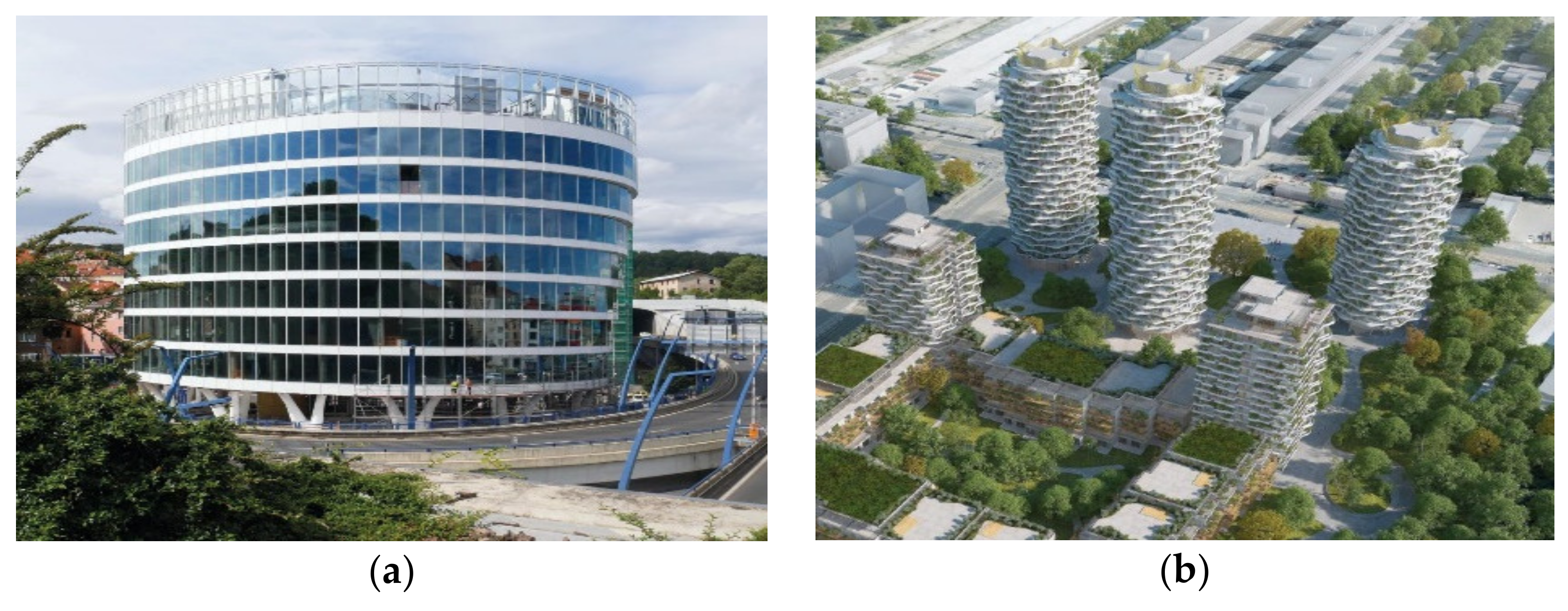
1. Introduction
2. Methods
2.1. Task Description
2.2. Numerical Model and Boundary Conditions
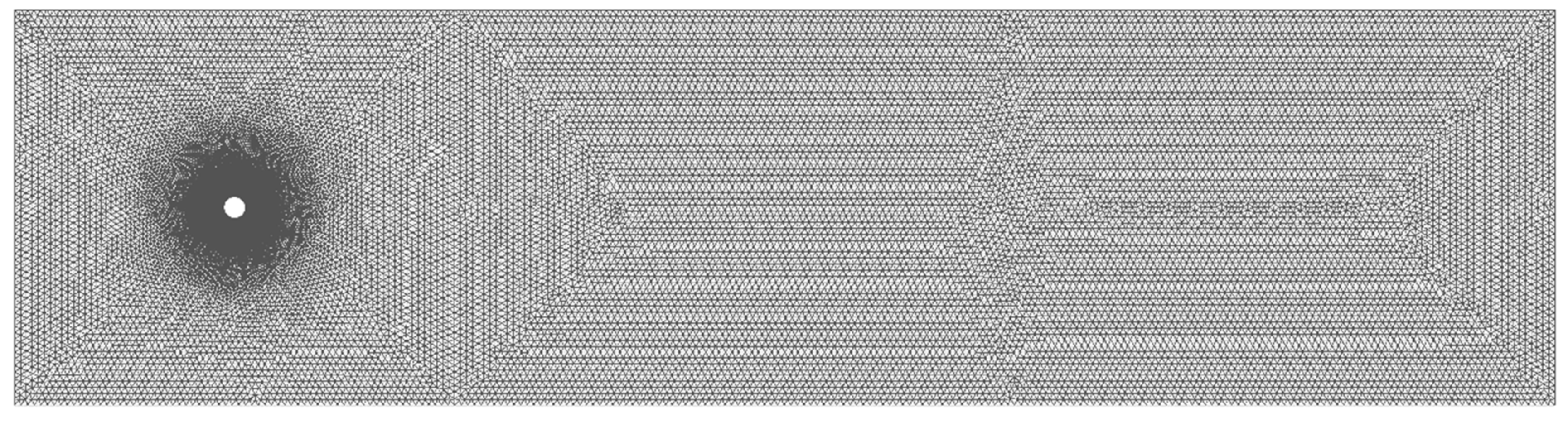
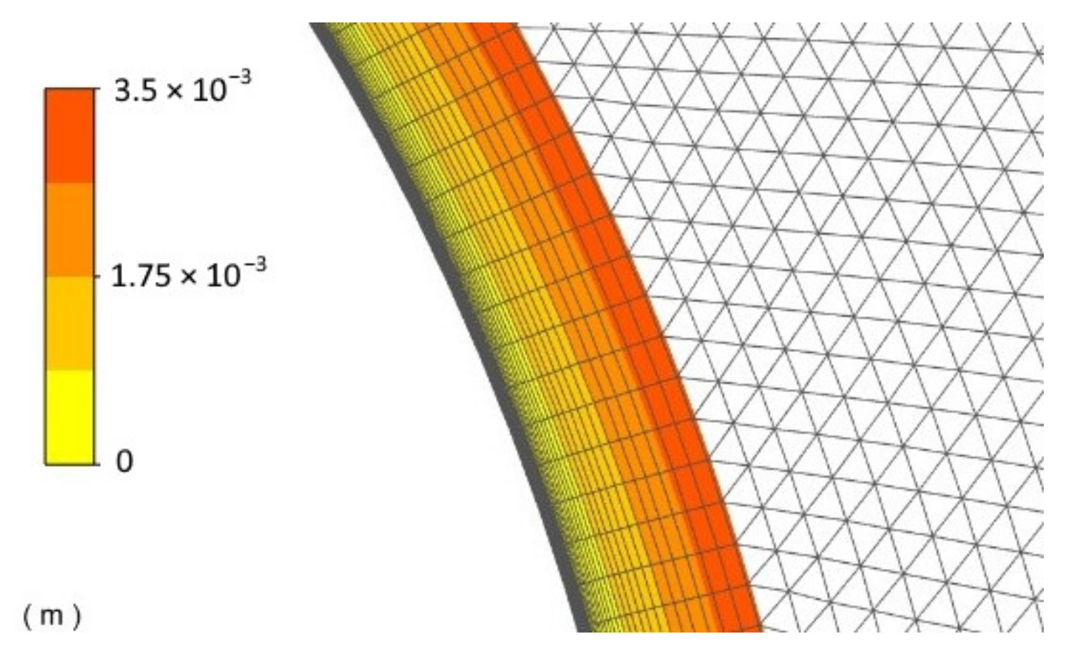
2.3. Meshing
3. Results
3.1. Flow Field Characteristics
3.1.1. Normalized Mean Stream Velocity in the Subcritical Region
3.1.2. Normalized Mean Stream Velocity in the Critical Region
3.2. Pressure Load on the Cylinder Circumference—Pressure Coefficient cp
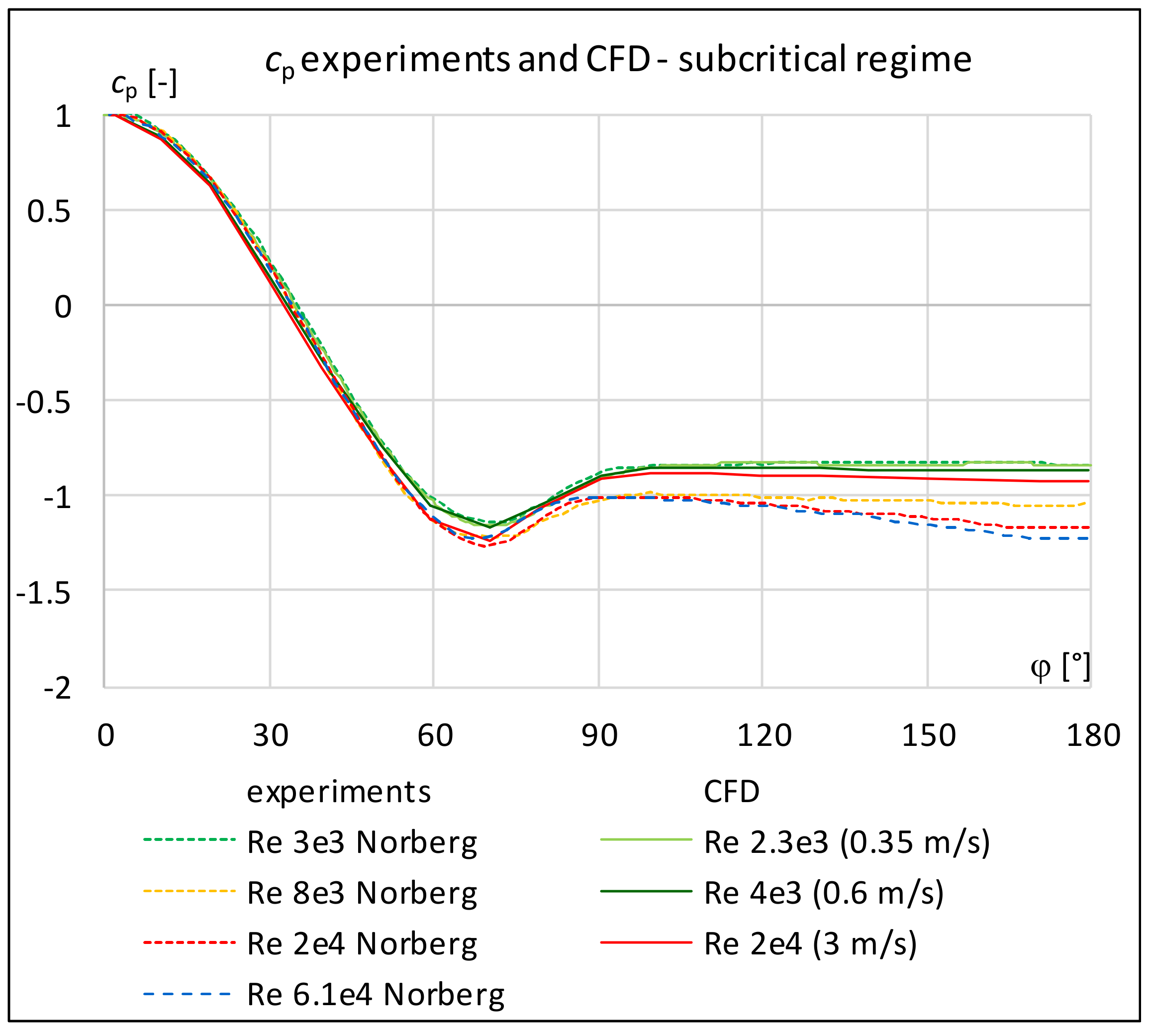
3.2.1. Pressure Coefficient cp—Subcritical Region
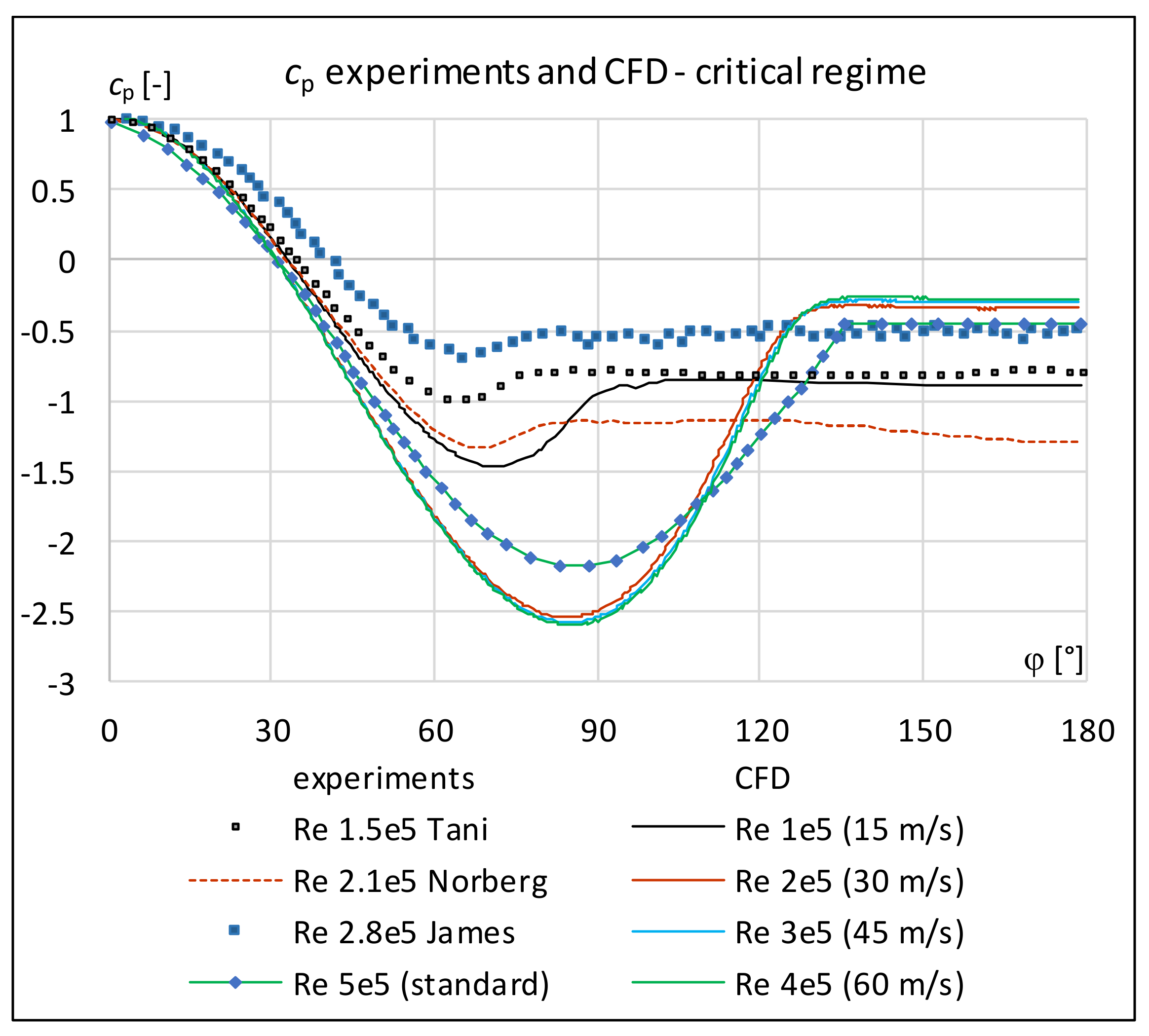
3.2.2. Pressure Coefficient cp—Critical Region, Re ≥ 1 × 10⁵
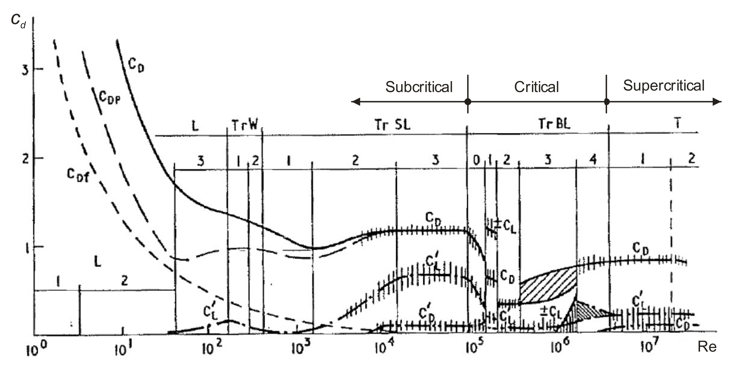
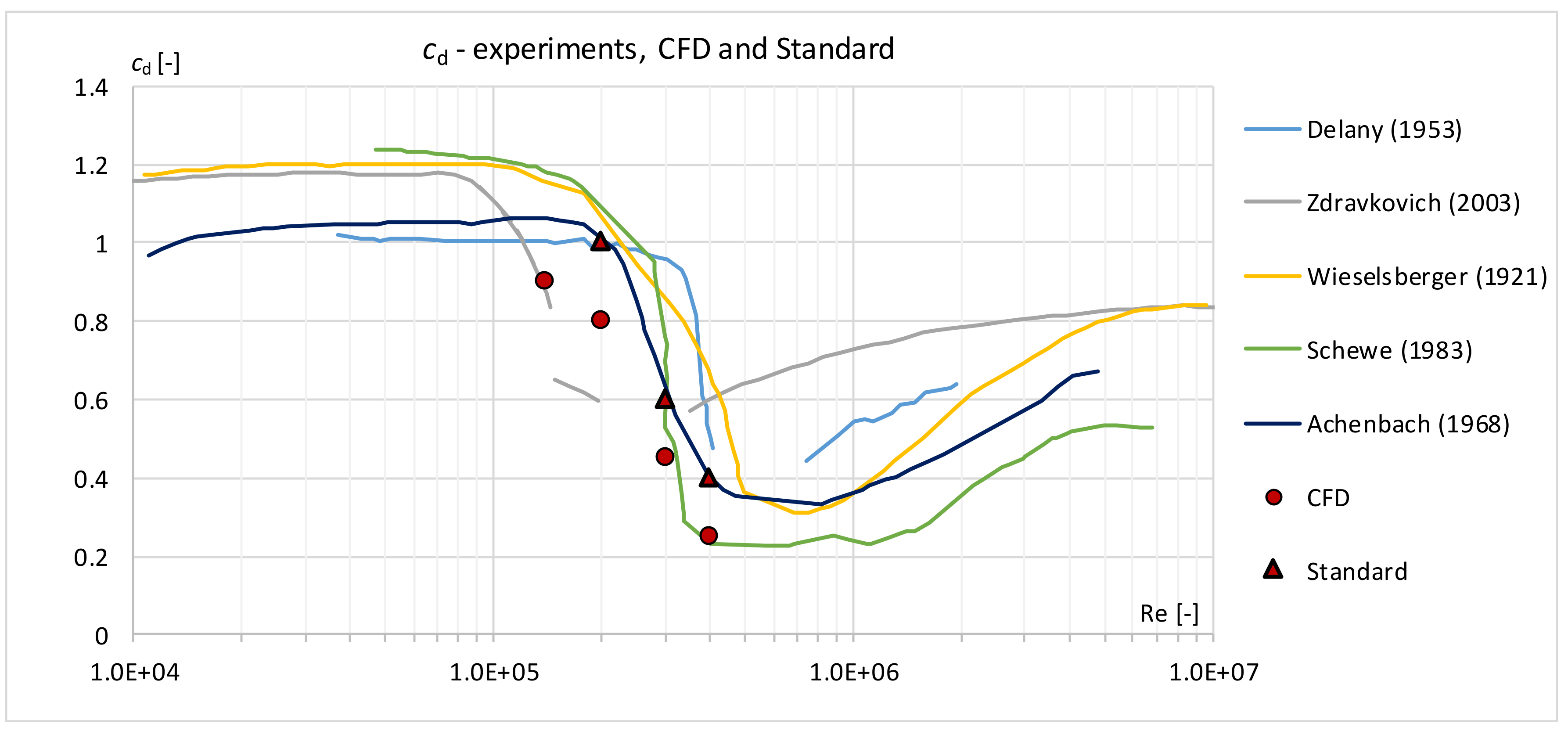
3.3. Drag Coefficient cd
4. Discussion
Author Contributions
Funding
Acknowledgments
Conflicts of Interest
References
- Blocken, B. Computational Fluid Dynamics for urban physics: Importance, scales, possibilities, limitations and ten tips and tricks towards accurate and reliable simulations. Build. Environ. 2015, 91, 219–245. [Google Scholar] [CrossRef]
- Toja-Silva, F.; Kono, T.; Peralta, C.; Lopez-Garcia, O.; Chen, J. A review of computational fluid dynamics (CFD) simulations of the wind flow around buildings for urban wind energy exploitation. J. Wind Eng. Ind. Aerodyn. 2018, 180, 66–87. [Google Scholar] [CrossRef]
- Michalcova, V.; Lausova, L. Numerical approach to determination of equivalent aerodynamic roughness of Industrial chimneys. Comput. Struct. 2017, 207, 187–193. [Google Scholar] [CrossRef]
- Ahlborn, B.; Seto, M.L.; Noack, B.R. On drag, Strouhal number and vortex-street structure. Fluid Dyn. Res. 2002, 30, 379–399. [Google Scholar] [CrossRef]
- Benidir, A.; Flamand, O.; Gaillet, L.; Dimitriadis, G. Impact of roughness and circularity-defect on bridge cables stability. J. Wind Eng. Ind. Aerodyn. 2015, 137, 1–13. [Google Scholar] [CrossRef]
- Matteoni, G.; Georgakis, C.T. Effects of bridge cable surface roughness and cross-sectional distortion on aerodynamic force coefficients. J. Wind Eng. Ind. Aerodyn. 2012, 104–106, 176–187. [Google Scholar] [CrossRef]
- Khashehchi, M.; Ashtiani Abdi, I.; Hooman, K. Characteristics of the wake behind a heated cylinder in relatively high Reynolds number. Int. J. Heat Mass Transf. 2015, 86, 589–599. [Google Scholar] [CrossRef]
- Kotrasova, K.; Kormanikova, E. The Study of Seismic Response on Accelerated Contained Fluid. Adv. Math. Phys. 2017, 2017, 1492035. [Google Scholar] [CrossRef]
- Jendzelovsky, N.; Antal, R.; Konecna, L. Determination of the wind pressure distribution on the facade of the triangularly shaped high-rise building structure. MATEC Web Conf. 2017, 107, 00081. [Google Scholar] [CrossRef]
- Hoxey, R.; Richards, P.; Robertson, A.; Quinn, A. Reynolds number effects on wind loads on buildings. In Proceedings of the 6th European and African Conference on Wind Engineering, EACWE 2013, Cambridge, UK, 7–11 July 2013. [Google Scholar]
- Medvecká, S.; Ivánková, O.; Macák, M. Pressure Coefficients Acting Upon the Cylinder Obtained by Numerical and Experimental Analysis. Civ. Environ. Eng. 2017, 13, 149–155. [Google Scholar] [CrossRef][Green Version]
- Medvecká, S.; Ivánková, O.; Macák, M.; Michalcová, V. Determination of Pressure Coefficient for a High-Rise Building with Atypical Ground Plan. Civ. Environ. Eng. 2018, 14, 138–145. [Google Scholar] [CrossRef]
- AI DESIGN—Centrum nového Žižkova “Living with Waves”. Available online: https://www.aidesign.cz/#/new-gallery-98/ (accessed on 9 November 2020).
- Ekologická Budova v Centru Prahy—Green Point | Konstrukce.cz. Available online: https://konstrukce.cz/architektura-a-development/ekologicka-budova-v-centru-prahy-green-point-170 (accessed on 9 November 2020).
- Patel, Y. Numerical Investigation of Flow Past a Circular Cylinder and in a Staggered Tube Bundle Using Various Turbulence Models. Master’s Thesis, Lappeenranta University of Technology, 2010. [Google Scholar]
- Abedin, Z.; Islam, M.Q.; Rizia, M.; Enam, H.M.K. A Review on the Study of Wind Loads on Multiple Cylinders with Effects of Turbulence and Surface Roughness. Am. J. Mech. Eng. 2017, 5, 87–90. [Google Scholar] [CrossRef]
- Zdravkovich, M.M. Flow around Circular Cylinders: A Comprehensive Guide through Flow Phenomena, Experiments, Applications, Mathematical Models, and Computer Simulations. Vol. 2: Applications; Oxford University Press: Oxford, UK, 2003; ISBN 0-19-856396-5. [Google Scholar]
- Cantwell, B.; Coles, D. An experimental study of entrainment and transport in the turbulent near wake of a circular cylinder. J. Fluid Mech. 1983, 136, 321. [Google Scholar] [CrossRef]
- Norberg, C. Pressure forces on a circular cylinder in cross flow. In Proceedings of the IUTAM Symposium Bluff-Body Wakes, Dynamics, and Instabilites, Göttingen, Germany, 7–11 September 1992; Springer: Berlin/Heidelberg, Germany, 1992; pp. 275–278. [Google Scholar]
- Schewe, G. On the force fluctuations acting on a circular cylinder in crossflow from subcritical up to transcritical Reynolds numbers. J. Fluid Mech. 1983, 133, 265–285. [Google Scholar] [CrossRef]
- Beaudan, P.; Moin, P. Numerical Experiments on the Flow Past a Circular Cylinder at Subcritical Reynolds Number; Thermosciences Division, Department of Mechanical Engineering, Stanford University: Stanford, CA, USA, 1994. [Google Scholar]
- Fröhlich, J.; Rodi, W.; Kessler, P.; Parpais, S.; Bertoglio, J.P.; Laurence, D. Large Eddy Simulation of Flow around Circular Cylinders on Structured and Unstructured Grids. In Numerical Flow Simulation I; Springer: Berlin/Heidelberg, Germany, 1998; pp. 319–338. [Google Scholar]
- Fu, C.; Zou, Z.; Liu, H.; Wang, Y.; He, X. Experimental study on the flow and heat transfer mechanism of the pre-cooler in the hypersonic aeroengine. In Proceedings of the 21st AIAA International Space Planes and Hypersonics Technologies Conference, Xiamen, China, 6–9 March 2017; American Institute of Aeronautics and Astronautics: Reston, VA, USA, 2017. [Google Scholar]
- Achenbach, E. Distribution of local pressure and skin friction around a circular cylinder in cross-flow up to Re = 5 × 10⁶. J. Fluid Mech. 1968, 34, 625–639. [Google Scholar] [CrossRef]
- Adachi, T.; Matsuuchi, K.; Matsuda, S.; Kawai, T. On the Force and Vortex Shedding on a Circular Cylinder from Subcritical up to Transcritical Reynolds Numbers. Bull. JSME 1985, 28, 1906–1909. [Google Scholar] [CrossRef][Green Version]
- Van Hinsberg, N.P. The Reynolds number dependency of the steady and unsteady loading on a slightly rough circular cylinder: From subcritical up to high transcritical flow state. J. Fluids Struct. 2015, 55, 526–539. [Google Scholar] [CrossRef]
- James, W.D.; Paris, S.W.; Malcolm, G.N. Study of Viscous Crossflow Effects on Circular Cylinders at High Reynolds Numbers. AIAA J. 1980, 18, 1066–1072. [Google Scholar] [CrossRef]
- Lehmkuhl, O.; Rodríguez, I.; Borrell, R.; Chiva, J.; Oliva, A. Unsteady forces on a circular cylinder at critical Reynolds numbers. Phys. Fluids 2014, 26, 125110. [Google Scholar] [CrossRef]
- Tani, I. Low-speed flows involving bubble separations. Prog. Aerosp. Sci. 1964, 5, 70–103. [Google Scholar] [CrossRef]
- Shur, M.L.; Spalart, P.R.; Strelets, M.K.; Travin, A.K. A hybrid RANS-LES approach with delayed-DES and wall-modelled LES capabilities. Int. J. Heat Fluid Flow 2008, 29, 1638–1649. [Google Scholar] [CrossRef]
- ČSN EN 1991-1-4ed. 2 Eurocode 1: Actions on Structures—Part 1-4: General Actions—Wind Loads, 2nd ed.; Úřad pro Technickou Normalizaci, Metrologii a Státní Zkušebnictví: Prague, Czech Republic, 2013.
- Yeon, S.M.; Yang, J.; Stern, F. Large-eddy simulation of the flow past a circular cylinder at sub- to super-critical Reynolds numbers. Appl. Ocean Res. 2016, 59, 663–675. [Google Scholar] [CrossRef]
- Delany, N.K.; Sorensen, N.E. Low-Speed Drag of Cylinders of Various Shapes; National Advisory Committee for Aeronautics: Washington, DC, USA, 1953; ISBN 9780874216561.


| Subcritical | Re = 2.3 × 10³ | Re = 4 × 10³ | Re = 2 × 10⁴ | ||
| u0 = 0.35 m·s−1 | u0 = 0.6 m·s−1 | u0 = 3 m·s−1 | |||
| Critical | Re = 1 × 10⁵ | Re = 1.4 × 10⁵ | Re = 2 × 10⁵ | Re = 3 × 10⁵ | Re = 4 × 10⁵ |
| u0 = 15 m·s−1 | u0 = 21 m·s−1 | u0 = 30 m·s−1 | u0 = 45 m·s−1 | u0 = 60 m·s−1 |
| Cylinder | D = 0.1 m | |
| Flowing medium—air | density (constant) kinematic viscosity dynamic viscosity | ρ = 1.225 kg·m−3 ν = 1.5 × 10⁻⁵ m2·s−1 μ = ν · ρ = 1.8 × 10⁻⁵ kg·(m·s)−1 |
| Boundary | Type of Boundary Condition |
|---|---|
| entry into computing area: | velocity inlet |
| output from computing area: | pressure outlet |
| vertical side walls: | symmetry: there is no friction on the side walls, the sides of the computational area do not affect the longitudinal velocity, the normal velocity and the flow of quantities across the border are zero |
| upper and lower horizontal walls: | wall: corresponds to wind tunnel conditions |
| cd—Subcritical Regime | cd—Critical Regime | |||||
|---|---|---|---|---|---|---|
| Re = 2.3 × 10³ | Re = 4 × 10³ | Re = 2 × 10⁴ | Re = 1.4 × 10⁵ | Re = 2 × 10⁵ | Re = 3 × 10⁵ | Re = 4 × 10⁵ |
| 1.05 | 1.02 | 1.02 | 0.90 | 0.82 | 0.45 | 0.25 |
Publisher’s Note: MDPI stays neutral with regard to jurisdictional claims in published maps and institutional affiliations. |
© 2021 by the authors. Licensee MDPI, Basel, Switzerland. This article is an open access article distributed under the terms and conditions of the Creative Commons Attribution (CC BY) license (http://creativecommons.org/licenses/by/4.0/).
Share and Cite
Kološ, I.; Michalcová, V.; Lausová, L. Numerical Analysis of Flow Around a Cylinder in Critical and Subcritical Regime. Sustainability 2021, 13, 2048. https://doi.org/10.3390/su13042048
Kološ I, Michalcová V, Lausová L. Numerical Analysis of Flow Around a Cylinder in Critical and Subcritical Regime. Sustainability. 2021; 13(4):2048. https://doi.org/10.3390/su13042048
Chicago/Turabian StyleKološ, Ivan, Vladimíra Michalcová, and Lenka Lausová. 2021. "Numerical Analysis of Flow Around a Cylinder in Critical and Subcritical Regime" Sustainability 13, no. 4: 2048. https://doi.org/10.3390/su13042048
APA StyleKološ, I., Michalcová, V., & Lausová, L. (2021). Numerical Analysis of Flow Around a Cylinder in Critical and Subcritical Regime. Sustainability, 13(4), 2048. https://doi.org/10.3390/su13042048