Abstract
Shipping trade and port operations are two of the primary sources of greenhouse gas emissions. The emission of air pollutants brings severe problems to the marine environment and coastal residents’ lives. Shore power technology is an efficient CO2 emission reduction program, but it faces sizeable initial investment and high electricity prices. For shipping companies, energy such as low-sulfur fuels and liquefied natural gas has become an essential supplementary means to meet emission reduction requirements. This research considers the impact of government subsidies on port shore power construction and ship shore power use. It constructs a multi-period dual-objective port shore power deployment optimization model based on minimizing operating costs and minimizing CO2 emissions. Multi-combination subsidy strategies, including unit subsidy rate and subsidy demarcation line, are quantitatively described and measured. The proposed Epsilon constraint method is used to transform and model the dual-objective optimization problem. Numerical experiments verify the effectiveness of the model and the feasibility of the solution method. By carrying out a “cost-environment” Pareto trade-off analysis, a model multi-period change analysis, and a subsidy efficiency analysis, this research compares the decision-making results of port shore power construction, ship berthing shore power use, and ship berthing energy selection. Government subsidy strategy and operation management enlightenment in the optimization of port shore power deployment are discussed.
1. Introduction
For a long time, sea transportation has been regarded as one of the most effective and safest means of transportation services. It has undertaken more than 80% of the international trade volume of goods [1]. Ports are the main gateways for international trade in goods and are vital to economic development around the world [2]. Simultaneously, the environmental pollution caused by ship berthing discharge, loading, and unloading operations have generated tremendous pressure on the green and sustainable development of the port [3]. The construction of green ports has received increasing attention under the strategic background of green development and green traffic flow.
When ships are at the port, auxiliary diesel engines are usually used to generate electricity to support ship production operations and people’s lives. During this period, diesel combustion will produce many greenhouse gases (GHG), sulfur dioxide (SO2), nitrogen oxides (NOx), particulate matter (PM), and other harmful pollutants, which are detrimental to the health of residents and ports in offshore areas. Sustainable development has brought an enormous impact [4]. According to related studies [5], 70% of the sulfur emissions from international shipping activities are concentrated along the main trade routes within 400 km of the coastline. For port cities with frequent shipping activities, the urban environmental impact caused by pollutant discharge is more significant [6].
To cope with the increasingly severe environmental pollution, the government and port companies strive to find solutions and have carried out active exploration and practice in port greening. Shore side electricity (SSE) is an effective measure to reduce port emissions. In 2008, the port in Stockholm, the capital of Sweden, designed and installed the world’s first high-voltage shore power system [7]. The so-called shore power technology is designed to stop using its auxiliary power generation system when the ship is berthing at the port, and then supply power to the shipboard system through the shore power grid or power source, so as to avoid the additional greenhouse gas and air pollutant emissions caused by the use of auxiliary diesel engines during the ship berthing at the port [8]. However, the deployment of shore power systems often requires port companies to bear more significant construction costs. In addition to the deployment of shoreline power facilities, liquefied natural gas (LNG), low-sulfur (0.5%) diesel, and other energy sources, while providing power output, produce fewer greenhouse gases or harmful gases than traditional diesel energy. Better environmental friendliness and lower cost of use make alternative energy sources another feasible solution to meet emission reduction requirements during ship stays [9].
The operation practice and theoretical research of green ports at home and abroad show that the government plays an essential role in promoting the green and sustainable development of ports [10]. The United States and Europe have successively proposed supporting policies to provide regulatory requirements and policy preferences to construct green ports and shipping [11]. The Californian government of the United States has formulated a timetable and route map for the use of shore power systems for ships calling at ports, requiring ships to use shore power when calling at ports with shore power facilities, and mandatory construction of ports that provide calling services for ships transporting a specified load. It is ultimately mandatory for shore power equipment that ships transporting specified loads must use shore power systems at ports of call [12]. Important European ports such as the Port of Amsterdam, the Port of Hamburg, the Port of Antwerp, and the Port of Rotterdam provide port taxes for ocean-going ships whose SOX, NOX, or CO2 emissions are lower than the industry average in accordance with the concessionary fees or tonnage fees of the International Maritime Organization (IMO) emission standards [13]. In 2018, the Ministry of Transport issued the Action Plan for Deepening the Construction of Green Ports (2018–2022) (Draft for Solicitation of Comments), which included port development concepts, energy consumption structure, recycling resources, strengthening pollution prevention, and innovative transportation methods in terms of in-depth promotion of green port construction [14].
At present, there are many studies on the deployment of green ports at home and abroad. Winkel et al. [15] quantified the economic and environmental potential of shore power construction in Europe. They put forward crucial obstacles and policy measures for implementing shore power policies by estimating in detail the emissions and related energy requirements of ships berthed. The U.S. Environmental Protection Agency (2017) [16] summarized 13 shore power studies in ports in the Americas, Europe, and Asia. It found that most ports have seen a 60% to 80% reduction in CO2 and pollutant emissions during the berthing period of container ships due to shore power systems. Wang et al. [17] comprehensively included cost reduction, energy-saving, and emission reduction goals and proposed a green port project scheduling model to optimize economic construction and complete environmental construction. Dai et al. [18] proposed a feasibility assessment framework for shore power investment that considers ecological factors, and carbon trading was also integrated into this framework. Wu and Wang [19] studied the issue of shore power deployment in containerships’ shipping networks. They proposed a government subsidy program to minimize the emissions of ships during berth. However, the literature mentioned above ignores the influence of government subsidy behavior’s key factor in the integrated optimization decision of port shore power construction and ship energy selection. In addition, through government subsidies, effectively alleviating the operational pressure of port companies and shipping companies can stimulate port companies and shipping companies to participate in the construction of green ports [20]. Maintaining a balance between cost control and environmental protection has also become an essential issue for green port construction [21].
Compared with the research conducted by Wu and Wang [19] that combined shore power deployment with container shipping network, this study focused on the deployment of shore power on port berths and considered the optimization of energy level and shore power level. This research constructs a mixed-integer programming optimization model for multi-period, bi-objective port shore power deployment. The proposed model integrates port shore power system deployment decisions, energy options for ship berthing, and government subsidy strategies. The government subsidy function implements a corresponding subsidy or penalty strategy according to the scale of port shore power construction and ship shore power cost. When the cost of port shore power construction or container ship power consumption is higher than a given value, the government will provide a specific cost subsidy. When the port shore power construction cost or ship shore power cost is lower than a given value, the government takes corresponding economic penalties.
In this research, the Epsilon constraint method is used to transform and solve the bi-objective problem. The influence of different government subsidy strategies and different environmental constraints on the optimal objectives of the model are investigated. The feasibility of the model and the solution method are verified through an example. Some management implications, such as strategy selection under different environmental constraints, are also obtained through corresponding numerical experiments.
2. Model Construction
2.1. Problem Description and Assumptions
This research analyzes the interactive relationship among the “government”, “port company”, and “shipping companies” in green port construction. The structure of the three-party interactive relationship is shown in Figure 1. Driven by passive policy requirements or active green transformations, port companies face the shore power construction’s decision-making to reduce CO2 emissions during ship stays in ports. Port companies shall make corresponding decision-making restrictions on using shore power systems or selecting auxiliary engine energy when the shipping company’s vessels are in port. The government grants port companies or shipping companies a certain number of subsidies based on the cost of port shore power construction or the cost of shore power usage during the ship stay in port to ease the cost pressure of participating in shore power construction.
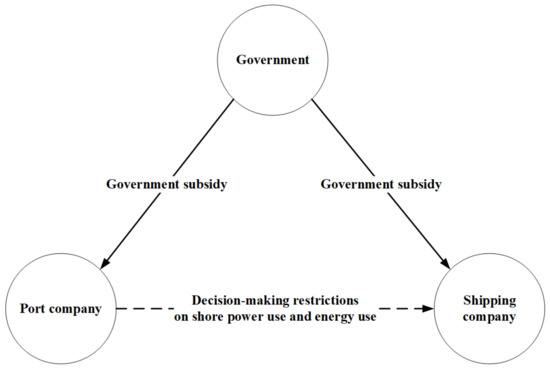
Figure 1.
The tripartite interaction of “government department–port company–shipping company” in the decision making of port shore power deployment.
The port shore power deployment problem proposed in this study considers the two optimization goals of cost control and environmental protection. Cost control mainly involves the construction cost of shore power, the energy consumption cost of ships’ stays in port, the cost of using shore power during ships’ stays in port, and possible subsidies or penalties from the government. In terms of environmental protection, this research mainly measures the CO2 emissions produced by energy use during ships’ stays in port. For convenience, this research only considers CO2 emissions as the only environmental impact factor. In addition, this research introduces different decision-making levels in the construction of port shore power and the energy selection of ships’ stays in port. The shore power facility level and energy cleanliness level can be set discretely [22]. For example, the shore power facility level can be set to “high”, “medium”, and “low”. These three levels correspond to three different construction costs and electricity costs. The energy cleanliness level can be set to “high”, “medium”, and “low”. These three levels correspond to three different energy consumption costs and CO2 emission levels. The higher the shore power system’s level, the lower the electricity cost per unit time for ships to stop, and the higher the corresponding construction cost. The higher the level of clean energy, the lower the amount of CO2 produced by ships per unit time of stoppage, and the higher the corresponding cost of use.
Therefore, this research designed the following dual-objective optimization content:
- (1)
- Minimize operating costs: operating costs including shore power construction costs, energy consumption costs for ships’ stays in ports, electricity costs for ships’ stays in ports, and government subsidies;
- (2)
- Minimize the environmental impact: minimization of CO2 emissions during ships’ stays in ports in the decision planning period.
Before the model is established, this section gives the following assumptions:
- (1)
- The port shore power construction is completed in the first phase of the decision-making plan.
- (2)
- Considering the influence of ship route planning, ship schedule delays, and other factors, the number of ships of a shipping company calling at a specific port in a single decision planning period is uniformly distributed on , namely,.
- (3)
- Considering the influence of factors such as differences in container loading and unloading operations, the time of a ship calling at a specific port in a single decision planning period is uniformly distributed on , namely,.
- (4)
- Assume that all ships at the port are of the same size and ignore the influence of ship inconsistency on the model decision.
2.2. Model Parameters and Decision Variable Settings
To provide a clearer introduction to the model, the following sub-section describes the model’s notation, parameters, decision variables, and objective functions, respectively. The interpretation of these symbols provides the basis for the construction of the model.
2.2.1. Notation
- the port, represents the set of all ports.
- the shore power level, represents the set of all shore power facility levels.
- the energy level, represents the set of all energy levels.
- the operating period, represents the set of all operating periods.
For example, represents the three-period port shore power construction cycle, and the measuring unit is based on one-year.
2.2.2. Parameter
- the construction cost of type shore power system.
- the cost of energy consumption per unit time when the ships use type energy.
- the cost of electricity consumption per unit time for ships of type shore power system to stay in port.
- the number of ships which visit port in period .
- the pollutant emissions (Kg) per unit period when ships use type energy.
- the average stay time (h) of the ships on each berthing at the port in the decision period .
- the number of berths in port .
- government subsidy (penalty) rate.
- demarcation limit of government subsidies for port shore power construction.
- demarcation limit of government subsidies for port shore power emission reduction.
- a large enough positive number.
2.2.3. Decision Variables
- The Boolean variable. If the port is carrying out the construction of the type shore power system, the value is 1. Otherwise, the value is 0.
- The port carries out the type shore power transformation construction scale for its berths, .
- In the decision period , port receives the number of ships that use type energy.
2.2.4. Objective Function
- Objective 1-cost objective function:
- Construction cost of shore power equipment
- Energy consumption cost for ships’ stay in port
- Electricity cost for ships’ stay in port
- Shore power construction subsidies
- Electricity subsidies for ships
- Objective 2-environment objective function:
- Total CO2 emission
2.3. Government Subsidy Function
The government subsidy functions, , can be set as piecewise functions, corresponding to the following three subsidy strategies [23].
Strategy S0: No subsidy and no penalty. The government does not subsidize the cost of port shore power construction or ship shore power consumption; that is, . This is shown in the first line of Equations (7) and (8).
Strategy S1: Only subsidize without penalty. The government subsidizes the cost of port shore power construction or ship shore power consumption and does not set a boundary subsidy (penalty) amount, and the unit subsidy rate is . That means . This is shown in the second line of Equations (7) and (8).
Strategy S2: There are subsidies and penalties. When the cost of port shore power construction or ship shore power consumption exceeds a certain amount, the subsidy will be given. Otherwise, it will be punished. The unit subsidy (penalty) rate is . That means, . This is shown in the third line of Equations (7) and (8).
2.4. Mathematical Model
The initial mathematical model is constructed as follows:
S.T.
Constraint condition (11) ensures that the scale of shore power construction in the port meets the demand for ships that use shore power systems and clean energy during their stay in port. Constraint condition (12) ensures that the shore power level for any port construction is unique. Constraint condition (13) provides that at least one port has implemented shore power construction. Constraints (14)–(15) ensure that the proportion of port shore power construction is valid only when the port decides to implement shore power construction. Constraints (16)–(18) define the variable.
3. Epsilon Constraint Solving Method
Epsilon constraint method is a frequently-used method to solve multi-objective optimization problems [24]. The basic idea of the solution method is [25]:
- (1)
- Selecting an objective function from multiple objective functions and listing it as the modified model’s single objective function based on the importance of the objective function and decision preference.
- (2)
- Constructing the Epsilon constraint problem by setting up the Epsilon constraint factor to transform the rest of the objective function into constraint conditions.
- (3)
- Solving the Epsilon constraint problem by gradually adjusting the value of the Epsilon constraint factor. In this research, the Epsilon constraint method is applied to solve the constructed dual-objective model, obtain the Pareto frontier, and analyze cost objective control and environmental objective control.
Due to the complexity of the cost objective function, this research sets it as the single objective after model transformation. Since the two objective functions are both minimization problems in the constructed mixed-integer programming model, the original model can be transformed into the following Epsilon constraint problem (Equation (9)).
S.T. (11)–(18)
Among the model mentioned above, is the Epsilon constraint factor (), is the maximum value of the original environmental target. The smaller the value of , the smaller the value of , indicating the higher the environmental requirements, and then restricting the upper limit of the environmental constraint of Equation (19). By adjusting the value of , the link between the cost objective and the environmental constraint can be established. can fix the original environmental objective as a single objective, and the fixed Equations (11)–(18) are the constraint, which is obtained by solving the maximum value of . Finally, the CPLEX solver is used to solve the constructed Epsilon constraint problem model .
Therefore, Epsilon constraint methods solving process for can be described, as shown in Algorithm 1.
| Algorithm 1 the Epsilon constraint method’s solving process |
 |
4. Numerical Experiment
4.1. Experiment Preparation
In the proposed model, the size of the optimization problem is set for the numerical experiment test to verify the feasibility of the constructed model and the Epsilon constraint method. This section uses five ports, several berths, and three planning periods. Each port is assigned a random number of berths, with varying numbers. According to the optimal decision of the proposed model, each berth in each port may be equipped with shore power equipment. The data in the literature [26,27] is applied as the basis to determine the relevant parameter settings of Section 2.2.2 listed in Table 1.

Table 1.
Input parameters related to the model.
The model is written in Visual Studio 2015 C#, the operating system is Windows 10 Professional X64, the processor is Intel Core (TM) i7-6500 @ 2.50 GHz, and the memory is 8 GB. Meanwhile, Visual Studio 2015 C# coding is used to call ILOG CPLEX 12.6.1.0, and CPLEX is used to solve the model.
4.2. Result Analysis
4.2.1. Comparison of Government Subsidy Strategies
Different government subsidy strategies often lead to different decision-making results. This section gives the strategy types under different parameter combinations. Different types of strategies are combined according to the unit subsidy rate and subsidy penalty threshold, as shown in Table 2. With Algorithm 1, this section calculates the different subsidy strategies listed in Table 2, and the Pareto curve of the result is shown in Figure 2.
Table 2.
Explanation of different subsidy strategies and codes.
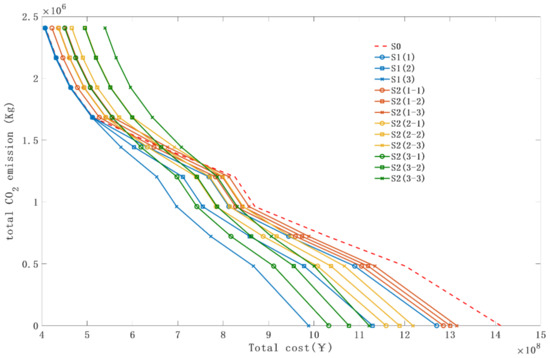
Figure 2.
Pareto curve under different government subsidy strategies.
The results in Figure 2 show that the Pareto curves reflected by different strategies are not the same. Overall, strategy S1(3) has the most significant effect. S1(3) has the least CO2 emission under the same cost, and S1(3) has the lowest cost under the same CO2 emission level. The reason for this result may be due to the higher unit subsidy rate a = 0.3. The S1(3) strategy requires the government to pay a higher cost of government subsidies, which eases port companies’ and shipping companies’ cost burden.
Viewed by sections, when the environmental constraints are small ( = 0.7, the left part of the abscissa in Figure 2), the effects of the S1(3) strategy and the S0 strategy are the same. In the decision-making problem of port shore power deployment, if the overall system’s environmental constraints are lower, it is appropriate to adopt the S0 strategy of no subsidies and no penalties, and there is no need to make government subsidies. As the environmental constraints gradually increase ( becomes smaller, the right part of the abscissa in Figure 2), the advantage of strategy S1(3) is reflected.
The internal comparison between the S1 series strategy and the S2 series strategy is also an evaluation direction that deserves attention. In the comparison of the S1 series strategy and the S2 series strategy, it is found that the larger the unit subsidy rate (), the more the Pareto curve shifts to the left, and the more significant the effect of the port shore power deployment decision. It is also in line with the port’s actual operation. In the internal comparison of the S2 series of strategies, it shows that the larger the unit subsidy rate (), the more the Pareto curve shifts to the left, and the more significant the effect of port shore power deployment decisions. However, the larger the quota standards represented by and , the more the Pareto curve shifts to the right. The reason may be that the larger the quota standard is, the greater the penalty imposed by the government on port companies and shipping companies for substandard on-shore power use will be, which leads to the rightist deviation of the Pareto curve. This result shows the effect of punitive government subsidies.
4.2.2. Comparison of Optimal Decision-Making Solutions and Sub-Objective Change
After strategy S1(3) was determined to be an ideal scheme, it is necessary to analyze the optimal solution composition and sub-objective changes in the strategy. Further, this part aims to understand the specific situation of the decision result and the main composition of the objective function value so that the port power construction has targeted implementation optimization and control. Table 3 shows the optimal solution of strategy S1(3) under different Epsilon constraints. Figure 3 shows the variation of the sub-target values of strategy S1(3) under different Epsilon constraints.
Table 3.
The optimal solution of strategy S1(3) under different Epsilon constraint factors.
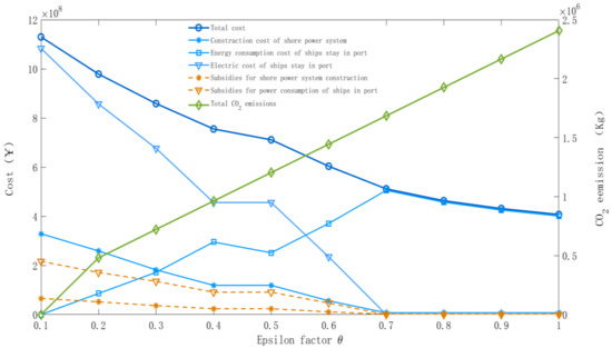
Figure 3.
The change of S1(3) strategy sub-objective value under different Epsilon constraint factors.
It can be found from Table 3 that when the Epsilon constraint factor is small ( = 0.1, 0.3, and 0.5), the level and scale of shore power construction are higher, and the ship energy utilization scale is lower. When the Epsilon constraint factor is large ( = 0.7, 0.9), the level and scale of shore power construction are low, and the level and scale of energy options for ship docking are higher.
Meanwhile, when the Epsilon constraint factor is small ( = 0.1 to = 0.5), the cost of electricity used by ships is the main cost factor. When the Epsilon constraint factor is large ( = 0.6 to = 1), the energy consumption cost of ships’ stays in port is the main cost factor.
The results in Table 3 and Figure 3 help discover the critical cost parameters under different environmental constraints: ship and port electricity costs are the crucial parameter under high environmental constraints. The ships’ energy consumption is the crucial parameter under low environmental constraints. The experimental results provide a basis for cost control under different scenarios and provide a reference for government decision makers to carry out targeted shore power construction and ship energy subsidies under different Epsilon constraint factors (i.e., various environmental constraints).
The results also show that when the Epsilon constraint factor is small (that is, the environmental constraints are strong), the port system’s CO2 emissions are low, and there are situations such as port shore power construction, ship shore power use, and ship energy use. From the perspective of increasing the proportion of shore power construction and improving the port’s environmental level, it is reasonable for many parties to place environmental constraints in the range of 0.1–0.6.
4.2.3. Analysis of the Efficiency of Environmental Improvement by Different Strategies of Government Subsidies
In discussing the changes in sub-objectives under different constraint conditions, another question worth discussing is: under different Epsilon constraint factors (that is, under environmental constraints), what kind of subsidy strategy allows the government to grant port shore power construction, and ship shore power use subsidies to improve the efficiency of the system’s environmental goals?
Here, referring to the value engineering theory (value = function/cost) [28], the formula for calculating the efficiency of government subsidies for improving the environment is given:
The ratio is calculated as the ratio of the reduction of CO2 emissions to government subsidies’ total input. The more significant environmental improvement and lower subsidy expenditures should be maintained to ensure higher improvement efficiency from the formula structure perspective.
Table 4 shows the efficiency values under different scenarios. It can be seen from Table 4 that when the Epsilon constraint factor is small (that is, the environmental constraint is large), , the S2(1-3) strategy has the highest efficiency value. While, the efficiency of each strategy type is the highest. When the Epsilon constraint factor is large (i.e., the environmental constraint is small, ), the efficiency value of the S2 strategy is the highest. The efficiency value of each strategy type is the highest while. Besides, when the Epsilon constraint factor is large, some strategies’ subsidy efficiency is also negative. Due to some strategies’ punitive measures, the government’s subsidy expenditure is negative (that is, a positive increase in revenue). Extensive environmental improvements and high subsidy penalties should be maintained to ensure high improvement efficiency in such situations.
Table 4.
Environmental improvement efficiency values of each subsidy strategy under different Epsilon constraint factors.
4.2.4. Comparison of Changes during the Decision-Making and Planning Period
The length of the decision-making planning period may affect the port shore power deployment decision. This part lists several Epsilon constraint factor scenarios () for three decision planning periods (short-term T = 3 years, medium-term T = 9 years, and long-term T = 27 years), and the change of the objective value is analyzed. The results are shown in Table 5.
Table 5.
The change of objective function value of strategy S1(3) under different Epsilon constraint factors and decision planning periods.
It can be found from Table 5 that the changes in the decision-making planning period mainly affect the energy consumption cost of ships’ stays in port () and the cost of electricity used by ships’ stays in port (), which in turn affects the government’s cost subsidies to shipping companies and the environmental objective. The short-term and mid-term decision-making and planning periods have no impact on the port shore power construction. Only in the partial Epsilon constraint factor (() scenario, the long-term decision-making, and planning period will have an impact on the cost of port shore power construction () and port shore power construction subsidies (). The experiment results remind decision-makers that it is necessary to pay attention to and control ships’ energy consumption cost and ships’ electricity cost in the long-term planning situation.
5. Discussion
Based on the background of green port construction activities, namely port shore power construction, shore power use, and ship energy use, this research constructs a port shore power deployment decision-making model considering government subsidies. The model minimizes operating costs and environmental impact as optimization objectives. The government subsidy functions, including subsidies and penalties, have been investigated. The Epsilon constraint method is used to transform and solve the bi-objective optimization model. Finally, a series of numerical experiments were carried out by calling the CPLEX solver to analyze and verify the proposed model and algorithm.
Experimental results show that:
- (1)
- From the perspective of ports and shipping companies, in the context of low environmental constraints (Epsilon constraint factor to ), the S0 strategy (no subsidies and no penalties) is an ideal solution for green port deployment. On the whole (Epsilon constraint factor to ), the S1(3) strategy that only subsidizes without penalty is an ideal solution.
- (2)
- When the environmental constraints are strong (Epsilon constraint factor to ), the cost of electricity used by ships is the main cost factor. When the environmental constraints are low (Epsilon constraint factor to ), the energy consumption cost of ships’ stays in port is the main cost factor. The results suggest that decision-makers need to select critical parameters for cost control under different environmental constraints.
- (3)
- When the environmental constraints are strong (that is, the Epsilon constraint factor is small), the port system’s CO2 emissions level is low, and the port shore power construction, ship shore power use, and ship energy use all exist. From the perspective of increasing the proportion of shore power construction and improving the port’s environmental level, it is reasonable to place environmental constraints in the range of 0.1–0.6 to participate in port shore power deployment.
- (4)
- The efficiency analysis of environmental improvement through different government subsidy strategies can help the government choose appropriate government subsidy strategies based on environmental constraints. The results show that when the environmental constraints are strong (that is, the Epsilon constraint factor is small), the S2(1-3) strategy is effective. When the environmental constraints are small (that is, the Epsilon constraint factor is large), the S1 strategy is effective.
- (5)
- The changes in the decision-making and planning period mainly affect the energy consumption cost of ships’ stays in port and the cost of electricity for ships’ stays in port. It is necessary to strengthen the cost control of both.
At this stage, this research only considers some of the decision-making factors for port shore power deployment. In the future, we will further study the integrated port shore power deployment issues, including complicated factors such as ship type changes [29] and port industrial integration [30].
Author Contributions
Conceptualization, H.L.; methodology, L.H.; validation, H.L.; formal analysis, L.H.; writing—original draft preparation, L.H.; writing—review and editing, L.H.; visualization, H.L. All authors have read and agreed to the published version of the manuscript.
Funding
This research received no external funding.
Institutional Review Board Statement
Not applicable.
Informed Consent Statement
Not applicable.
Data Availability Statement
Not applicable.
Conflicts of Interest
The authors declare no conflict of interest.
References
- Arvis, J.F.; Ojala, L.; Wiederer, C.; Shepherd, B.; Raj, A.; Dairabayeva, K.; Kiiski, T. Connecting to Compete 2018: Trade Logistics in the Global Economy; World Bank: Washington, DC, USA, 2018. [Google Scholar]
- Qu, X.; Meng, Q. The economic importance of the Straits of Malacca and Singapore: An extreme-scenario analysis. Transp. Res. Part E Logist. Transp. Rev. 2012, 48, 258–265. [Google Scholar] [CrossRef]
- Zhen, L.; Hu, Z.; Yan, R.; Zhuge, D.; Wang, S. Route and speed optimization for liner ships under emission control policies. Transp. Res. Part C Emerg. Technol. 2020, 110, 330–345. [Google Scholar] [CrossRef]
- IMO. Third IMO GHG Study 2014; International Maritime Organization (IMO): London, UK, 2014. [Google Scholar]
- Zhen, L.; Zhuge, D.; Murong, L.; Yan, R.; Wang, S. Operation management of green ports and shipping networks: Overview and research opportunities. Front. Eng. Manag. 2019, 6, 152–162. [Google Scholar] [CrossRef]
- Yu, J.; Voß, S.; Tang, G. Strategy development for retrofitting ships for implementing shore side electricity. Transp. Res. Part D Transp. Environ. 2019, 74, 201–213. [Google Scholar] [CrossRef]
- Zis, T.P. Prospects of cold ironing as an emissions reduction option. Transp. Res. Part A Policy Pract. 2019, 119, 82–95. [Google Scholar] [CrossRef]
- Kotrikla, A.M.; Lilas, T.; Nikitakos, N. Abatement of air pollution at an aegean island port utilizing shore side electricity and renewable energy. Mar. Policy 2017, 75, 238–248. [Google Scholar]
- Martínez-Moya, J.; Vazquez-Paja, B.; Maldonado, J.A.G. Energy efficiency and CO2 emissions of port container terminal equipment: Evidence from the Port of Valencia. Energy Policy 2019, 131, 312–319. [Google Scholar] [CrossRef]
- Lam, J.S.L.; Li, K.X. Green port marketing for sustainable growth and development. Transp. Policy 2019, 84, 73–81. [Google Scholar] [CrossRef]
- Aregall, M.G.; Bergqvist, R.; Monios, J. A global review of the hinterland dimension of green port strategies. Transp. Res. Part D Transp. Environ. 2018, 59, 23–34. [Google Scholar]
- Di Vaio, A.; Varriale, L. Management innovation for environmental sustainability in seaports: Managerial accounting instruments and training for competitive green ports beyond the regulations. Sustainability 2018, 10, 783. [Google Scholar] [CrossRef]
- Radwan, M.E.; Chen, J.; Wan, Z.; Zheng, T.; Hua, C.; Huang, X. Critical barriers to the introduction of shore power supply for green port development: Case of Djibouti container terminals. Clean Technol. Environ. Policy 2019, 21, 1293–1306. [Google Scholar]
- Wu, X.; Zhang, L.; Yang, H.C. Integration of eco-centric views of sustainability in port planning. Sustainability 2020, 12, 2971. [Google Scholar] [CrossRef]
- Winkel, R.; Weddige, U.; Johnsen, D.; Hoen, V.; Papaefthimiou, S. Shoreside electricity in Europe: Potential and environmental benefits. Energy Policy 2016, 88, 584–593. [Google Scholar] [CrossRef]
- Vaishnav, P.; Fischbeck, P.S.; Morgan, M.G.; Corbett, J.J. Shore power for vessels calling at US ports: Benefits and costs. Environ. Sci. Technol. 2016, 50, 1102–1110. [Google Scholar] [CrossRef] [PubMed]
- Wang, W.; Huang, L.; Gu, J.; Jiang, L. Green port project scheduling with comprehensive efficiency consideration. Marit. Policy Manag. 2019, 46, 967–981. [Google Scholar] [CrossRef]
- Dai, L.; Hu, H.; Wang, Z.; Shi, Y.; Ding, W. An environmental and techno-economic analysis of shore side electricity. Transp. Res. Part D Transp. Environ. 2019, 75, 223–235. [Google Scholar]
- Wu, L.; Wang, S. The shore power deployment problem for maritime transportation. Transp. Res. Part E: Logist. Transp. Rev. 2020, 135, 101883. [Google Scholar] [CrossRef]
- Tseng, P.H.; Pilcher, N. Evaluating the key factors of green port policies in Taiwan through quantitative and qualitative approaches. Transp. Policy 2019, 82, 127–137. [Google Scholar] [CrossRef]
- Demir, E.; Hrušovský, M.; Jammernegg, W.; Van Woensel, T. Green intermodal freight transportation: Bi-objective modeling and analysis. Int. J. Prod. Res. 2019, 57, 6162–6180. [Google Scholar] [CrossRef]
- Zhen, L.; Huang, L.; Wang, W. Green and sustainable closed-loop supply chain network design under uncertainty. J. Clean. Prod. 2019, 227, 1195–1209. [Google Scholar]
- Wang, Z.; Huang, L.; He, C.X. A multi-objective and multi-period optimization model for urban healthcare wastes reverses logistics network design. J. Comb. Optim. 2019, 1, 1–28. [Google Scholar]
- Huang, L.; Murong, L.; Wang, W. Green closed-loop supply chain network design considering cost control and CO2 emission. Mod. Supply Chain Res. Appl. 2020, 2, 42–59. [Google Scholar] [CrossRef]
- Laumanns, M.; Thiele, L.; Zitzler, E. An efficient, adaptive parameter variation scheme for metaheuristics based on the epsilon-constraint method. Eur. J. Oper. Res. 2006, 169, 932–942. [Google Scholar] [CrossRef]
- Wan, C.; Zhang, D.; Yan, X.; Yang, Z. A novel model for the quantitative evaluation of green port development—A case study of major ports in China. Transp. Res. Part D Transp. Environ. 2018, 61, 431–443. [Google Scholar] [CrossRef]
- Peng, Y.; Li, X.; Wang, W.; Wei, Z.; Bing, X.; Song, X. A method for determining the allocation strategy of on-shore power supply from a green container terminal perspective. Ocean Coast. Manag. 2019, 167, 158–175. [Google Scholar] [CrossRef]
- Belton, V. A comparison of the analytic hierarchy process and a simple multi-attribute value function. Eur. J. Oper. Res. 1986, 26, 7–21. [Google Scholar] [CrossRef]
- Dere, C.; Deniz, C. Load optimization of central cooling system pumps of a container ship for the slow steaming conditions to enhance the energy efficiency. J. Clean. Prod. 2019, 222, 206–217. [Google Scholar] [CrossRef]
- Huang, L.; Zhen, L.; Yin, L. Waste material recycling and exchanging decisions for industrial symbiosis network optimization. J. Clean. Prod. 2020, 276, 124073. [Google Scholar] [CrossRef]


Publisher’s Note: MDPI stays neutral with regard to jurisdictional claims in published maps and institutional affiliations. |
© 2021 by the authors. Licensee MDPI, Basel, Switzerland. This article is an open access article distributed under the terms and conditions of the Creative Commons Attribution (CC BY) license (http://creativecommons.org/licenses/by/4.0/).